Article

A Parallel Computing Approach to Gene Expression and Phenotype Correlation for Identifying Retinitis Pigmentosa Modifiers in Drosophila

1
Department of Computer Science, Purdue University Fort Wayne, Fort Wayne, IN 46805, USA
2
Department of Biology, Purdue University Fort Wayne, Fort Wayne, IN 46805, USA
*
Author to whom correspondence should be addressed.
Computation 2023, 11(6), 118; https://doi.org/10.3390/computation11060118
Submission received: 16 May 2023 / Revised: 5 June 2023 / Accepted: 6 June 2023 / Published: 14 June 2023
(This article belongs to the Special Issue Computational Biology and High-Performance Computing)

Abstract

:
As a genetic eye disorder, retinitis pigmentosa (RP) has been a focus of researchers to find a diagnosis through either genome-wide association (GWA) or RNAseq analysis. In fact, GWA and RNAseq are considered two complementary approaches to gaining a more comprehensive understanding of the genetics of different diseases. However, RNAseq analysis can provide information about the specific mechanisms underlying the disease and the potential targets for therapy. This research proposes a new approach to differential gene expression (DGE) analysis, which is the heart of the core-analysis phase in any RNAseq study. Based on the Drosophila Genetic Reference Panel (DGRP), the gene expression dataset is computationally analyzed in light of eye-size phenotypes. We utilized the foreach and the doParallel R packages to run the code on a multicore machine to reduce the running time of the original algorithm, which exhibited an exponential time complexity. Experimental results showed an outstanding performance, reducing the running time by 95% while using 32 processes. In addition, more candidate modifier genes for RP were identified by increasing the scope of the analysis and considering more datasets that represent different phenotype models.

1. Introduction

Retinitis pigmentosa (RP) is a genetic eye disorder that causes progressive degeneration of the cells in the retina, leading to significant visual impairment or blindness in some cases. RP is caused by mutations in genes that are essential for the normal functioning of the retina, and there are several different genetic forms of the disorder. There is currently no cure for RP, but there are treatments that can help manage the symptoms and slow the progression of the disease [1].
Recent studies on the human genetic database show a significant comparability between Drosophila Melanogaster, commonly known as the fruit fly, and human genes. Thus, the Drosophila Genetic Reference Panel (DGRP) was created in 2007, which includes a standardized set of over 200 inbred lines and more than 20,000 annotated genes. It provides a powerful resource for geneticists and evolutionary biologists to investigate, in a controlled setting, the genetic basis of a wide range of traits including behaviors, morphology, and disease susceptibility [2,3]. For example, by exposing the DGRP strains to environmental conditions that mimic the effects of RP, such as exposure to light-induced oxidative stress, researchers can observe differences in the severity and progression of the disease across the different strains.
Through genome-wide association (GWA) studies, researchers can then identify genetic variants that are significantly associated with disease as well as potential targets for therapeutic intervention. In their GWA, Chow et al. [4] identified 100 candidate genes that were linked to retinal degeneration and may play a role in the progression of RP. However, this type of analysis cannot fully identify potential modifiers that are indirectly related to changes in eye size and may be differentially regulated several steps downstream of the associated gene. In this case, RNAseq analysis can be used in ways that are complementary to GWA to investigate the genetics of RP [5]. While GWA focuses on identifying genetic variants associated with the disease, RNAseq analysis can be used to investigate the effects of these variants on gene expression and pathway dysregulation [6]. This provides insights into the specific mechanisms underlying the disease and potential targets for therapy. Additionally, RNAseq analysis can be used to validate the functional relevance of genetic variants identified by GWA [7].
As explained by Conesa et al. [5], differential gene expression (DGE) analysis is the heart of the core-analysis phase in any RNAseq study. Various techniques have been developed to evaluate expression data among multiple samples and identify suspect genes. Some of the methods rely on specific discrete probability distributions, such as the Poisson and negative binomial distributions [8]. edgeR is a comprehensive package in R that takes raw read data and carries out both normalization and differential expression analysis simultaneously [9]. More packages, including baySeq [10] and EBseq [11], on the other hand, follow the Bayesian negative binomial paradigm to identify differential gene expression. Furthermore, methods such as NOISeq [12] and SAMseq [13] are non-parametrically designed and introduce fewer false premises and estimations based on existing data. In a comparative study by Soneson and Delorenzi [14], several DGE approaches were investigated using simulated and real RNA-seq data. The results showed that all methods performed better for large sample sizes using more than three samples per condition for an RNA-seq experiment. EBSeq showed the strongest dependency on the sample size while DESeq offered the best results for smaller sample size datasets.
An alternative approach would be observing extreme phenotypes (such as extremely large or small eye sizes) and trying to understand how they are linked to changes in gene expression when they are significantly altered in strains. Although this approach has been used successfully to identify modifier genes in a variety of diseases and cancers [15,16], it has not yet been widely applied to Drosophila. Two previous studies investigated candidate RP genes using eye-size phenotypes and the gene expression level of DGRP. Amstutz et al. [17] utilized the unsupervised learning algorithm of K-Mean clustering to group strains based on the profile of their expression levels. The extreme minimum and maximum eye-size profiles were selected from a total of six clusters. The two replicates for each selected line were averaged and passed to the differential gene expression analysis algorithm. The study further validated the RP candidate genes by comparing the control eye sizes with RNA interference (RNAi) strains.
On the other hand, Nguyen et al. [18] proposed selecting sixteen strains that exhibit extreme eye size and generating a list of all their possible replicate combinations instead of using the average expression value between two replicates of a DGRP strain. The “best combination” is then selected, such that only the strain replicate that offers the best expression/eye-size correlation among all the genes is selected and considered for further analysis. However, the main issue is the intensive computations required to find the best replicate, especially when considering a large number of strains.
The objective of this research is to speed up the execution time of Nguyen’s approach by exploiting some parallel computing constructs in the R language. Hence, the main contributions are (1) restructuring the code to run in parallel on a multicore processor, (2) filtering out the input datasets before the analysis, and (3) using the p-value to assess the statistical significance of the results. The rest of the paper is organized as follows: Section 2 describes the structure of the input datasets and the steps of the proposed computational approach. In Section 3, the results of the study are presented and discussed in the light of several experiments considering different performance criteria. Potential candidate modifiers are then identified and their relation to eye development and degeneration are highlighted in Section 4. Finally, Section 5 summarizes the conclusions as well as some future research directions.

2. Materials and Methods

2.1. Input Datasets

As the goal of this research was to explore the correlation between the genotype of RP and the phenotype of degenerative eye-size, we needed two types of datasets. The first is the DGRP gene expression dataset which was developed by Huang et al. [19], measuring the expression levels for 185 DGRP strains over 18,140 genes. As shown in Table 1, this dataset is represented by a matrix with the genes as rows and the DGRP stains as columns. The gene names have the FBgn/XLOC prefix followed by an identification number. In fact, the FBgn genes have been recognized and fully annotated in Flybase, while little is known about the XLOC genes. In addition, the values stored in the matrix cells are the RNA expression value for each strain. With two replicates for each strain line, the columns are annotated using the postfix “:1” and “:2” representing the first and the second replicate, respectively.
The eye-size phenotype, on the other hand, is captured by three different datasets: Rh1G69D, rpr, and p53. Those resulted from studies that observed different apoptosis (programmed cell death)-induced retinal degeneration models across the DGRP. Chow et al. [4] studied the Rh1G69D model of degeneration, representing 173 DGRP lines. Overexpression of p53 or reaper (rpr) were both studied by Palu et al. [20]. The 204 strains from the DGRP were used for the GMR > p53 study and 202 were used for the GMR-rpr study. The average two-dimensional eye area was measured for at least 10 female flies that were flash-frozen prior to imaging. The eye area is defined as the area of the polygon connecting certain landmark points around the eye. Usually, the eye area is manually measured using tools such as Adobe Photoshop on frontal images of the head [21]. As shown in Table 2, the three datasets are saved in a text file that contains two columns: strain IDs and the average eye size measured in pixels × 103. A strain ID comprises an indicator, “RAL”, followed by a three-digit identification number. It is also worth noting that some strains in eye-size datasets don’t exist in the expression-level matrix. Hence, only the intersection between the two will be analyzed in each case.

2.2. Correlation Analysis

The correlation coefficient is used in the fields of science and finance to statistically assess the relationship between two variables, factors, or datasets. Its values can range from −1 to 1, where −1 indicates a perfect inverse correlation, with values in one series rising as those in the other decline, and vice versa. A value of 1 shows a perfect direct correlation, and the value 0 means there is no linear relationship. Although Pearson’s formula is the most commonly used correlation method, it cannot assess nonlinear associations between variables or those arising from sampled data not subject to a normal distribution. In these cases, nonparametric methods such as Spearman’s, the Kendall rank, or a polychronic correlation coefficient can be used to analyze the relationships.
Pearson’s correlation is a covariance between two samples divided by product of the standard deviation of those samples. The covariance and standard deviation can be calculated by using Equations (1) and (2), respectively. Then, we can use those equations to obtain the correlation coefficient as shown in Equation (3). The variables x i and y i are the specific values in a sample, while x and y are the mean of each sample. Additionally, variable n is the number of values contained in a sample.
c o v x , y = 1 n 1 i = 1 n x i x × y i y
S D x = x i x 2 n 1
r x , y = c o v x , y S D x × S D y = i = 1 n x i x × y i y x i x 2 × y i y 2
The vectors x and y represent the average eye sizes being analyzed and the expression values of a specific gene, respectively. n, on the other hand, corresponds to the number of strains being selected for this iteration of calculation. Furthermore, since correlation does not imply causation, a correlation analysis is usually followed by a statistical significance test using the p-value, which allows us to assess the level of significance of the correlation calculation [22].

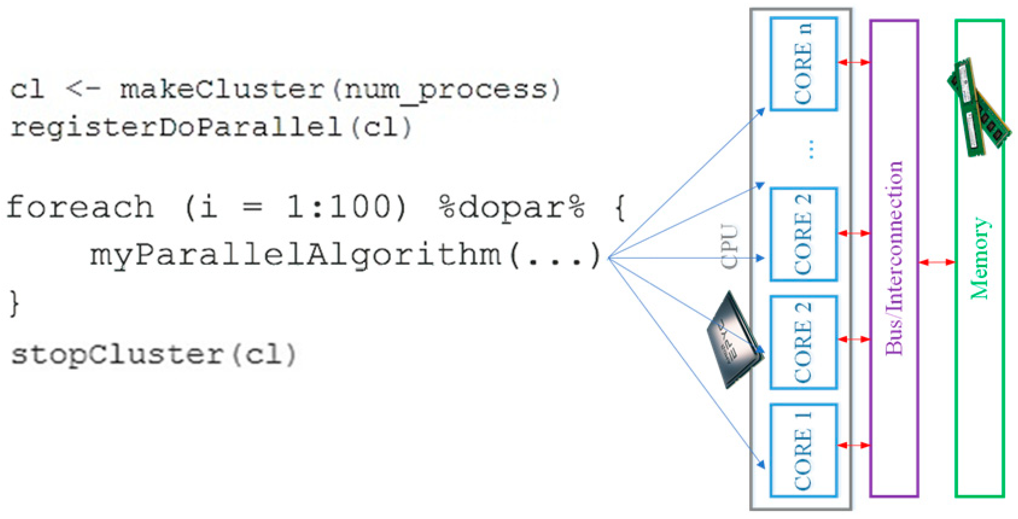
2.3. Parallel Computation in R

Unlike C/C++ or Fortran, R has not been designed to run in parallel. Although its basic packages are highly optimized for sequential programs, it still requires a long time to process huge datasets. Therefore, several packages have been developed, and made available on CRAN, to facilitate parallel processing of R code. The doParallel package, for example, uses a data parallelization scheme to spread computational tasks onto multiple processing cores of a non-clustered architecture with a shared-memory paradigm. doParallel is not a stand-alone package but operates jointly with three other packages: parallel, foreach, and iterators. The parallel package provides the basis for process creation and termination on both UNIX-based and Windows operating systems. In a similar fashion to the parallel package for openMP, the foreach package is used to distribute the data onto multiple CPU cores and consolidate the results from each process by applying an appropriate function [23].
As shown in Figure 1, the doParallel functions makeCluster, registerDoParallel, and stopCluster are used to manage the parallel region creation and termination. The %dopar% enables the loop to be parallelized through foreach, where each CPU core executes a chunk of the loop’s iteration space. In fact, foreach and doParallel packages can be executed in both serial and parallel modes by toggling the .inorder parameter, which should be TRUE for serials and FALSE for parallels.

2.4. The Computational Approach

The algorithms mapping phenotypes to associated RP genotypes using eye-size and DGRP gene expression data were originally proposed by Nguyen et al. [18]. In fact, a huge barrier towards extending their analysis was the intensive computational requirements of the algorithms. Hence, the main contribution of this research is to use a parallel computing approach to improve performance and reduce the overall execution time.
The main steps of the computations are summarized in Algorithm 1. In addition to the two datasets, it receives bottom and top quantile values as inputs. Those values, in turn, determine the strains representing the largest and the smallest eye-size groups. In fact, small eye sizes reflect the phenotype related to the RP genes while healthy eyes are characterized by large sizes. The quantile values can be adjusted so that the number of strains selected from each extreme eye-size group are balanced.
Since the input data come from two different sources (eye-size and expression level datasets), we will focus on those strain lines that are shared between the two datasets in each case. That is, non-intersecting strain lines will be discarded by the pre-processing step prior to applying the steps of the main algorithm. In addition, after a careful inspection of the expression level dataset, we found that some lines are represented with only one replicate. Those were filtered out as well and were not considered in the subsequent steps.
Once the extreme strains are identified and selected, Algorithm 2 is executed to generate the matrix of all possible replicate combinations for the selected lines. Since each strain has two replicates, the algorithm encodes each replicate combination with a binary number and decides which replicate to choose based on the values of their corresponding binary digit. Based on the number of selected extreme strains (N), the algorithm encodes the numbers from 0 to 2N−1. For example, in the case of 6 selected strains, the total number of possible replicate combinations is 64 (26). The first generated number will be 000000, which selects the first replicate of every strain. Next, the sequence 100000 selects the second replicate of the first strain and the first replicate of the other five. The following numbers will be 010000, 110000, 001000, 101000, …… etc. The last combination will be represented by 111111, which means that the second replicate of each strain is selected.
It is clear that Algorithm 3 takes the longest time to run because the number of possible combinations grows exponentially with the number of selected lines, not to mention the huge size of the DGRP expression dataset. The sequential time complexity of the method can be expressed using (4), where N refers to the number of selected lines representing extreme eye sizes and G represents the number of genes in the gene expression dataset. When dividing this workload across p processes, the parallel execution time can be expressed by (5). The impact of using parallel processing will be investigated and discussed more in the Results section.
T s = 2 N × G
T p = T s p
Note that, beside the memory allocated for the two datasets, the space requirements of this algorithm include the matrix holding the replicate combinations and the vectors storing the list of candidate genes, as well as their correlation coefficients and their corresponding p-values. The space complexity of the proposed method can be estimated by (6), where L and G represent the number of lines and genes in the DGRP expression dataset, respectively.
S p a c e   C o m p l e x i t y = L × G + L × 2 + 2 N × N + G × 3
Algorithm 1. Main Algorithm
Input:
Aes—Average eye sizes
Expr—Expression-level matrix
low_quantile—Bottom quantile of eye sizes
high_quantile—Top quantile of eye sizes
C—Correlation threshold value
num_process—Number of parallel processes
Output:
 List of candidate genes
Begin
 Filterout strains in Expr with only one replicate.
 Filterout strains in Expr with no matching values in Aes.
selSizes ⟵ eye sizes in Aes less than low_quantile or greater than high_quantile values
extreme_strains ⟵ strains in Aes corresponding to selSizes
rep_combsAlgorithm2 (extreme_strains)
best_rep_combAlgorithm3 (selSizes, Expr, rep_combs, C, num_ process)
candidate_genesAlgorithm4 (SelSizes, Expr, rep_combs, best_rep_comb, C)
Print candidate_genes, their correlation coefficients, and p-values.
End
Algorithm 2. Generate replicate combinations
Input:
selStrain—Selected extreme strains.
Output:
replicate_comb—Replicate combinations matrix.
Begin
N ⟵ Length(selStrain)
for i ⟵ 1 to 2N do
  binary ⟵ DecimalToBinary(i)
  for every binary digit d at position j in binary do
   if d is 0 then
    replicate_comb[i] ⟵ first replicate of strain j
   else
    replicate_comb[i] ⟵ second replicate of strain j
return replicate_comb
End
Algorithm 3. Find the best replicate combination
Input:
selSizes—Average eye sizes of selected strains
 Expr—Expression level matrix
 replicate_comb—Replicate combinations matrix
 C—Correlation threshold value
 num_process—Number of parallel processes
Output:
 bestCombination—Best replicate combination
Begin
 Create a parallel team with num_process processes.
 Let scoreVec and combVec be empty vectors.
foreach replicate combination c[i] in replicate_comb do
for every gene j do
   Score ⟵ 0
   selExprs[j] ⟵ expression levels of j in the selected combination c[i]
   temp[j] ⟵ correlation value between selExprs[j] and selSizes
   if temp[j] < -C OR temp[j] > C then
      ScoreScore + 1
    end
end
  Append Score to ScoreVec
  Append c[i] to combVec
end
 Terminate the parallel session.
bestCombination ⟵ Replicate combination in combVec associated with Max(ScoreVec)
return bestCombination
End
Algorithm 4. Find candidate genes
Input:
selSizes—Average eye sizes of selected strains
Expr—Expression level matrix
best_rep_comb—Best replicate combination
C—Correlation threshold value
Output:
sorted_genes—List of candidate genes with their correlation coefficients and p-values
Begin
 Let m be the number of genes in Expr
 Let Results be a list of length m
foreach gene j do
  Results[j] ⟵ correlation coefficient and p-values of selSize and gene expression levels of j
    for best_rep_comb in Expr
end
 Filterout genes in Results’ with p-values less than 0.05
 Filterout genes in Results’ with correlation coefficients not in the range [C, 1] nor [−1, -C]
 sorted_genes ⟵ Sort Results’ in descending order based on the absolute values of correlation
      s coefficients
return sorted_genes
End
Among all the generated combinations, Algorithm 3 tries to find the best combination based on their correlation with the average eye-size values. That is, for each replicate combination, the vector of expression levels of one gene is correlated with the vector of average eye-sizes for the selected extreme strains. When the absolute value of the calculated correlation coefficient exceeds the set threshold, it contributes to the total score of that replicate combination. Based on these accumulated scores, the best combination is determined as the one achieving the highest score. Obviously, as the number of selected extreme lines increases, the number of replicate combinations grows exponentially. Therefore, when implementing Algorithm 3 we utilized the parallel computing constructs in R to cut down the execution time. More discussion will be given in the results section.
The final step of the analysis is handled by Algorithm 4, which calculates the Pearson’s correlation coefficients between all genes in the best replicate combination and extreme eye sizes. The algorithm also computes the p-value in each case, and those correlations with p-values greater than or equal to 0.05 are filtered out of the list of candidate genes. The same is done with genes whose absolute correlation coefficient values don’t exceed the set threshold value. Finally, Algorithm 1 should print out the sorted list of candidate genes along with their correlation coefficients and p-values.

3. Results

3.1. Experimental Setup

3.1.1. Datasets

The analysis here is primarily based on the DGRP expression level dataset, which consists of 368 columns representing 185 different Drosophila strain lines and 18,140 rows of genes. Each strain line has two replicates except for RAL513 and RAL890, which have one replicate each. Thus, when excluding these lines, the expression dataset has 6,675,520 expression values in total. On the other hand, the eye-size datasets of Rh1G69D, rpr, and p53 consist of 173, 202, and 204 strains, respectively. As discussed above, we will focus only on those strains that intersect with the DGRP expression dataset. Table 3 shows the detailed statistics of the three eye-size datasets. For example, Rh1G69D has 170 filtered strains with an arithmetic mean of 21,540.20 × 103 pixels.

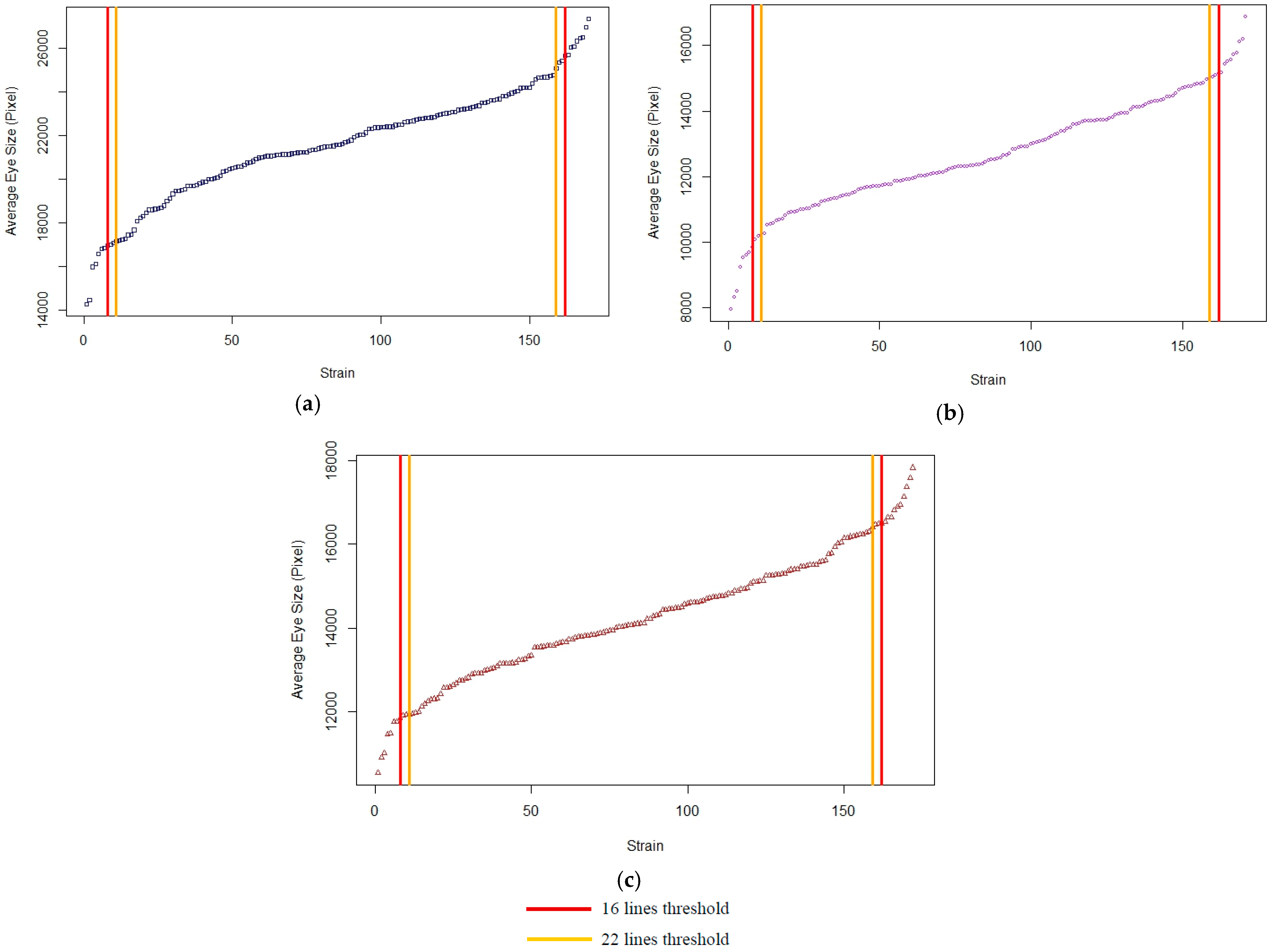
3.1.2. Quantile Thresholds

To investigate the effect of changing the number of selected lines representing the extreme eye sizes in the results, we need to find adequate quantile threshold values for each case. More specifically, we will investigate groups of 16, 18, 20, and 22 lines while trying to maintain a balanced number of strains representing extremely small and large eye sizes within a group. Table 4 lists the threshold values utilized for each group in the three datasets. Figure 2 depicts the cutoff lines for the 16- and 22-line groups using red and yellow colors, respectively, where the eye-size data is sorted in an ascending order. In the case of the 16-line group, for example, the selected strains are those that appear on the left and the right of the left and the right red cutoff lines, respectively.

3.1.3. Hardware & Software Specifications

To implement the set of proposed algorithms, the R scripting language version 4.2.1 was used. In addition, several external libraries were utilized to analyze the data and support parallel computations. For example, cor() and cor.test() functions from the stats package were used to perform the correlation analysis step. The doParallel (ver. 1.0.17) package was used to facilitate parallelism on loops through the foreach (ver. 1.5.2) package. The original version of the code, initially developed by Nguyen et al. [18], used the highly optimized sapply and lapply sequential functions from the R base package.
The experiments were initially deployed on a laptop, then on the Diamond server of the department of computer science, Purdue University Fort Wayne. The laptop runs 64-bit Windows 8.1 on an Intel i7-6700HQ (sixth generation) CPU with a base clock speed of 2.6 GHz and 8 GB of RAM. The Diamond server runs the Oracle Linux operating system version 8.7 on AMD EPYC 7452 CPU with a base clock speed of approximately 2.3 GHz and 62 GB of RAM. While the laptop has four cores with eight physical threads, the Diamond server has thirty-two cores and can manage up to sixty-four threads.

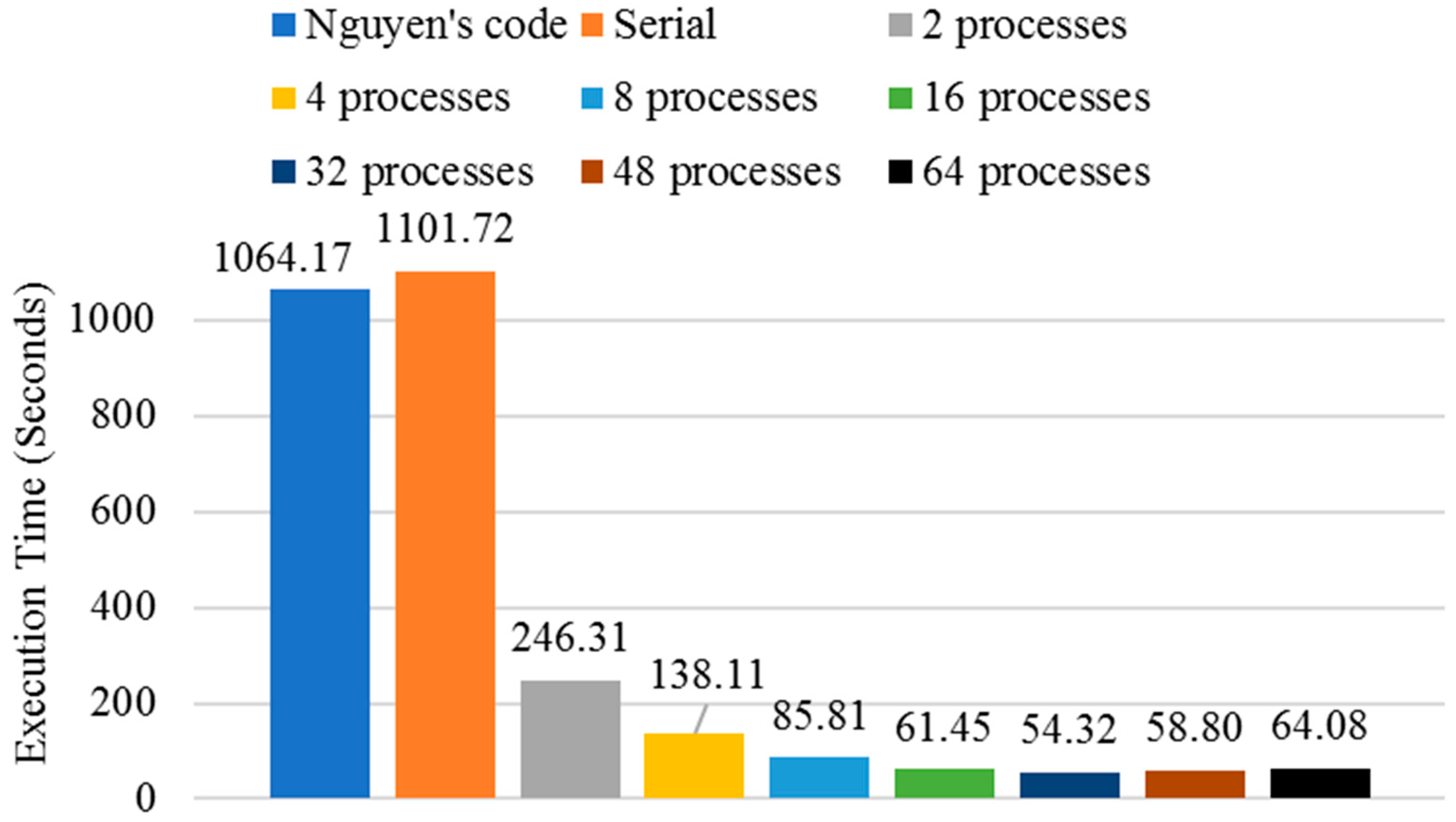
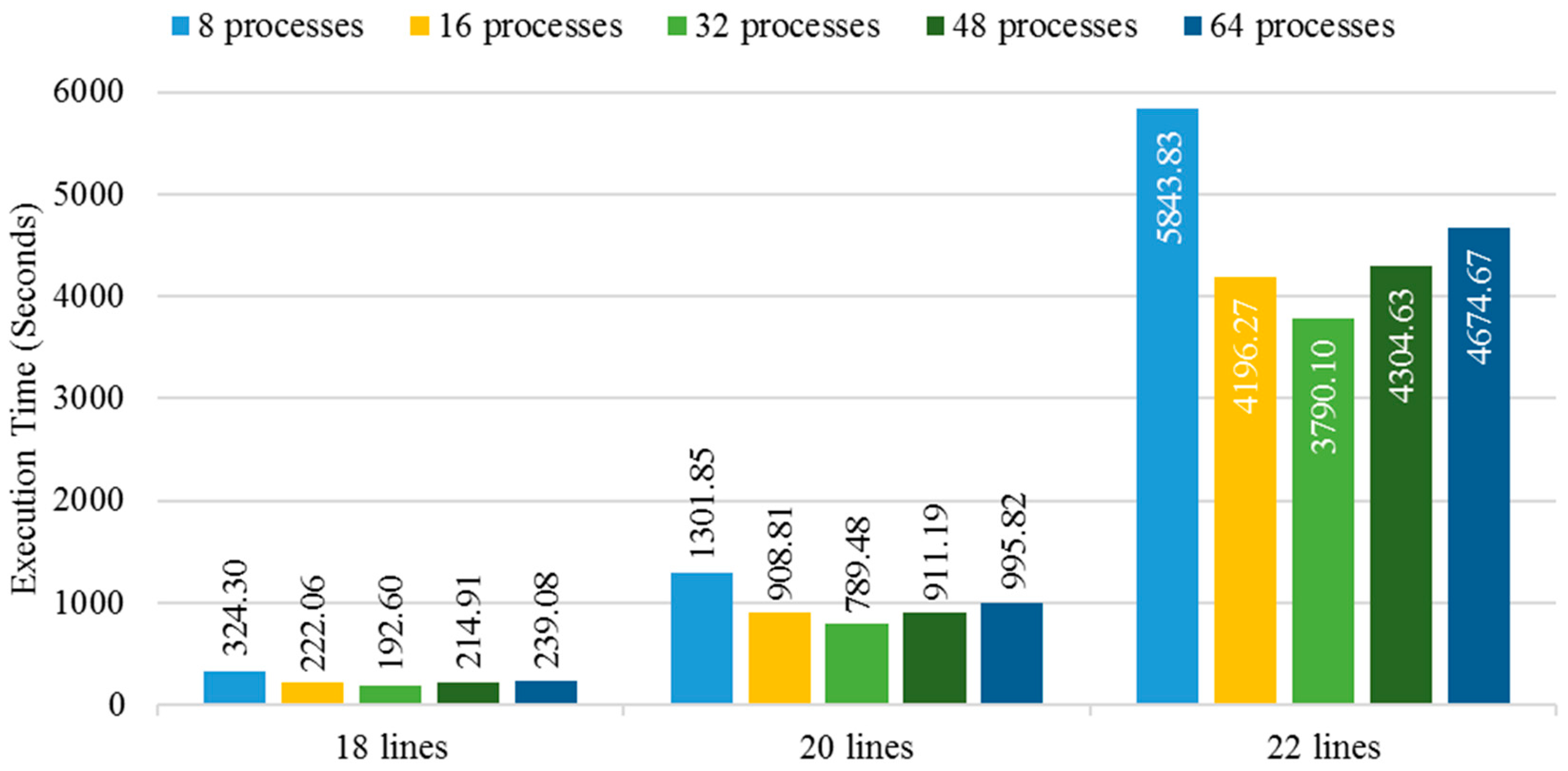
3.2. Execution Time Analysis

In this set of experiments, the execution time of each algorithm was tested on the laptop for sixteen strain lines of the Rh1G69D eye-size dataset. Nguyen’s original code was compared with the enhanced parallel implementation. Table 5 shows the measured execution time for each algorithm separately. The results show that there is a clear overhead when executing Algorithm 2 in parallel, and recommend the used of the sequential sapply function in the following experiments. Similarly, we recommend running Algorithm 4 for eight processes, since the increase in speed achieved when moving from four to eight processes was not significant and further increases in the number of processes may cause overhead. Algorithm 3, on the other hand, showed an outstanding speedup since it was originally the most time consuming one. In fact, the number of possible replicate combinations increases drastically with increasing the number of selected lines. For example, using 16 lines in this case, 65,536 (216) different correlation calculations are needed for each gene. With 22 lines, the number of possible combinations reaches 222 or 4,194,304.
Using the Diamond server, we were able to repeat the same experiment using the recommended parameters for Algorithm 2 and Algorithm 4 while increasing the number of processes running Algorithm 3. Figure 3 depicts the average execution time for ten runs using sixteen lines from the Rh1G69D eye-size dataset. The results clearly show the outstanding performance of the proposed parallel solution compared to Nguyen’s version, even when only two threads were used. Furthermore, the results show that the best performance was achieved with 32 processes, with a roughly 95% decrease in execution time when compared to the sequential version. Using more than 32 processes showed a slight overhead that affected the execution time. To further investigate the optimal setting for Algorithm 3, we repeated the same set of experiments considering more lines in the extreme eye-size groups. The results shown in Figure 4 confirm that the execution time when using 32 processes is consistently lower than other settings regardless of the number of selected lines.

3.3. Suspected Candidate Genes

Here, we are going to focus only on the top ten candidate modifiers that exhibit the highest correlation values with the extreme eye sizes for each of the three eye-size datasets. The complete list of genes will be provided as supplementary material (Tables S1–S12). The top candidate RP genes for the Rh1G69D dataset using 16, 18, 20, and 22 strain lines are listed in Table 6. Table 7 and Table 8 show the top genes for the rpr and p53 datasets, respectively. The suspect genes that carry over at least three groups of selected lines are highlighted in blue. Those are potentially significant and worth further investigation. For example, the gene FBgn0032847 appeared in all four groups of the Rh1G69D dataset and has the highest correlation values in both the 20 and 22 groups. The same is true for the genes FBgn0027601 and FBgn0053017 in the rpr dataset and FBgn0004373 in the p53 dataset. Furthermore, the gene FBgn0037770 was found to be a common suspect gene between Rh1G69D and p53, and FBgn0015024 existed in both lists of rpr and p53.

4. Discussion

We will focus our discussion here on top correlated RP genes that appeared at least three times in different line groups or across different eye-size datasets. Based on this criteria, 16 genes have been identified and are listed in Table 9. The table shows the actual gene names, symbols, and their human orthologs (the human genes that share the same functionality as the Drosophila genes). Some of these genes have potential connections to apoptosis/disease, which are briefly described in the last column.
This list of candidate modifiers is completely distinct from the results discussed in both Chow’s [4] and Amstutz’s [17] due to the different approaches implemented for the DGE analysis. However, when compared with Nguyen’s top ten candidate genes [18], two intersecting genes were identified: MORF-related gene 15 (MRG15) and p (pink). However, the relationship of these candidate genes with the degenerative retinal disease cannot be validated until further in-depth biological lab experiments.

5. Conclusions

In this study, we have improved the algorithm for finding candidate RP genes originally proposed by Nguyen [18]. The method starts with identifying extreme eye-size strains and generating an exhaustive list of their possible replicate combinations. The best replicate combination is then identified as the one maximizing the correlation between the eye-size phenotype and the expression profiles of all genes. With 2N possible replicate combinations considered for each gene in the dataset, the sequential implementation of the method was found to be time consuming, which limited the number of lines (N) that could be considered and hence the scope of the analysis.
Therefore, we have implemented a parallel version of the method using the foreach and the doParallel R packages. This enabled the program to run faster than the original version and decreased the execution time by up to 95% when using 32 processes. Moreover, beside the DGRP gene expression dataset, three eye-size datasets, Rh1G69D, rpr, and p53, were also considered. Several experiments have been conducted on groups of 16, 18, 20, and 22 extreme lines. In our analysis, we focused on the top ten candidate genes, giving a particular importance to those genes which emerged over multiple groups of selected lines and/or datasets. As a result, sixteen candidate genes were identified and need to be further validated through a follow up biological study to prove their association with the RP disease.
Future directions for this work could be extending the focus of analysis beyond the top ten candidate genes. In addition, given access to more powerful computational resources, the experiments could include groups with more than 22 extreme lines. Another extension could be applying a standard DGE analysis tool, such as DESeq2, to the expression data for the best replicate combination. One can also consider rewriting the code using other languages such as C/C++ and use GPUs for a more efficient parallel implementation.

Supplementary Materials

The following supporting information can be downloaded at: https://www.mdpi.com/article/10.3390/computation11060118/s1, Table S1: The list of all valid genes for 16-lines of Rh1G69D, Table S2: The list of all valid genes for 18-lines of Rh1G69D, Table S3: The list of all valid genes for 20-lines of Rh1G69D, Table S4: The list of all valid genes for 22-lines of Rh1G69D, Table S5: The list of all valid genes for 16-lines of rpr, Table S6: The list of all valid genes for 18-lines of rpr, Table S7: The list of all valid genes for 20-lines of rpr, Table S8: The list of all valid genes for 22-lines of rpr, Table S9: The list of all valid genes for 16-lines of p53, Table S10: The list of all valid genes for 18-lines of p53, Table S11: The list of all valid genes for 20-lines of p53, Table S12: The list of all valid genes for 22-lines of p53.

Author Contributions

Conceptualization, A.K.; Data curation, C.M.; Formal analysis, R.P.; Methodology, A.K.; Project administration, A.K.; Resources, R.P.; Software, C.M.; Visualization, C.M.; Writing—original draft, A.K.; Writing—review & editing, C.M. and R.P. All authors have read and agreed to the published version of the manuscript.

Funding

This research received no external funding.

Data Availability Statement

Genomic sequence and gene expression data for the DGRP is available at http://dgrp.gnets.ncsu.edu/ (accessed on 4 June 2023). Gene expression data was initially published in Huang et al. 2015. Eye size data is available as a supplementary file from Show et al. 2016. Code can be provided upon request.

Acknowledgments

This research was part of a Master thesis research in Computer Science at Purdue University Fort Wayne. We would like to thank the department for facilitating the access to the Diamond Server to run the parallel experiments during the period January to May 2023.

Conflicts of Interest

The authors declare no conflict of interest.

References

  1. Hartong, D.T.; Berson, E.L.; Dryja, T.P. Retinitis pigmentosa. Lancet 2006, 368, 1795–1809. [Google Scholar] [CrossRef] [PubMed]
  2. Huang, W.; Massouras, A.; Inoue, Y.; Peiffer, J.; Ràmia, M.; Tarone, A.M.; Turlapati, L.; Zichner, T.; Zhu, D.; Lyman, R.F.; et al. Natural variation in genome architecture among 205 Drosophila melanogaster Genetic Reference Panel lines. Genome Res. 2014, 24, 1193–1208. [Google Scholar] [CrossRef] [PubMed] [Green Version]
  3. Mackay, T.F.C.; Richards, S.; Stone, E.A.; Barbadilla, A.; Ayroles, J.F.; Zhu, D.; Casillas, S.; Han, Y.; Magwire, M.M.; Cridland, J.M.; et al. The Drosophila melanogaster Genetic Reference Panel. Nature 2012, 482, 173–178. [Google Scholar] [CrossRef] [PubMed] [Green Version]
  4. Chow, C.Y.; Kelsey, K.J.P.; Wolfner, M.F.; Clark, A.G. Candidate genetic modifiers of retinitis pigmentosa identified by exploiting natural variation in Drosophila. Hum. Mol. Genet. 2016, 25, 651–659. [Google Scholar] [CrossRef] [PubMed] [Green Version]
  5. Conesa, A.; Madrigal, P.; Tarazona, S.; Gomez-Cabrero, D.; Cervera, A.; McPherson, A.; Szcześniak, M.W.; Gaffney, D.J.; Elo, L.L.; Zhang, X.; et al. A survey of best practices for RNA-seq data analysis. Genome Biol. 2016, 17, 13. [Google Scholar] [CrossRef] [Green Version]
  6. Karademir, D.; Todorova, V.; Ebner, L.J.A.; Samardzija, M.; Grimm, C. Single-cell RNA sequencing of the retina in a model of retinitis pigmentosa reveals early responses to degeneration in rods and cones. BMC Biol. 2022, 20, 86. [Google Scholar] [CrossRef] [PubMed]
  7. Li, J.; Du, W.; Xu, N.; Tao, T.; Tang, X.; Huang, L. RNA-Seq Analysis for Exploring the Pathogenesis of Retinitis Pigmentosa in P23H Knock-In Mice. Ophthalmic Res. 2021, 64, 798–810. [Google Scholar] [CrossRef]
  8. Robinson, M.D.; Smyth, G.K. Moderated statistical tests for assessing differences in tag abundance. Bioinformatics 2007, 23, 2881–2887. [Google Scholar] [CrossRef] [Green Version]
  9. Robinson, M.D.; McCarthy, D.J.; Smyth, G.K. edgeR: A Bioconductor package for differential expression analysis of digital gene expression data. Bioinformatics 2010, 26, 139–140. [Google Scholar] [CrossRef] [Green Version]
  10. Hardcastle, T.J.; Kelly, K.A. baySeq: Empirical Bayesian methods for identifying differential expression in sequence count data. BMC Bioinform. 2010, 11, 422. [Google Scholar] [CrossRef] [Green Version]
  11. Leng, N.; Dawson, J.A.; Thomson, J.A.; Ruotti, V.; Rissman, A.I.; Smits, B.M.G.; Haag, J.D.; Gould, M.N.; Stewart, R.M.; Kendziorski, C. EBSeq: An empirical Bayes hierarchical model for inference in RNA-seq experiments. Bioinformatics 2013, 29, 1035–1043. [Google Scholar] [CrossRef] [PubMed] [Green Version]
  12. Tarazona, S.; García-Alcalde, F.; Dopazo, J.; Ferrer, A.; Conesa, A. Differential expression in RNA-seq: A matter of depth. Genome Res. 2011, 21, 2213–2223. [Google Scholar] [CrossRef] [PubMed] [Green Version]
  13. Li, J.; Tibshirani, R. Finding consistent patterns: A nonparametric approach for identifying differential expression in RNA-Seq data. Stat. Methods Med. Res. 2013, 22, 519–536. [Google Scholar] [CrossRef] [PubMed] [Green Version]
  14. Soneson, C.; Delorenzi, M. A comparison of methods for differential expression analysis of RNA-seq data. BMC Bioinform. 2013, 14, 91. [Google Scholar] [CrossRef] [PubMed] [Green Version]
  15. Liang, P.; Pardee, A.B. Analysing differential gene expression in cancer. Nat. Rev. Cancer 2003, 3, 869–876. [Google Scholar] [CrossRef] [PubMed]
  16. Rodriguez-Esteban, R.; Jiang, X. Differential gene expression in disease: A comparison between high-throughput studies and the literature. BMC Med. Genom. 2017, 10, 59. [Google Scholar] [CrossRef] [Green Version]
  17. Amstutz, J.; Khalifa, A.; Palu, R.; Jahan, K. Cluster-Based Analysis of Retinitis Pigmentosa Modifiers Using Drosophila Eye Size and Gene Expression Data. Genes 2022, 13, 386. [Google Scholar] [CrossRef]
  18. Nguyen, T.; Khalifa, A.; Palu, R. Identifying Genes Related to Retinitis Pigmentosa in Drosophila melanogaster Using Eye Size and Gene Expression Data. BioMedInformatics 2022, 2, 625–636. [Google Scholar] [CrossRef]
  19. Huang, W.; Carbone, M.A.; Magwire, M.M.; Peiffer, J.A.; Lyman, R.F.; Stone, E.A.; Anholt, R.R.H.; Mackay, T.F.C. Genetic basis of transcriptome diversity in Drosophila melanogaster. Proc. Natl. Acad. Sci. USA 2015, 112, E6010–E6019. [Google Scholar] [CrossRef] [Green Version]
  20. Palu, R.A.S.; Ong, E.; Stevens, K.; Chung, S.; Owings, K.G.; Goodman, A.G.; Chow, C.Y. Natural Genetic Variation Screen in Drosophila Identifies Wnt Signaling, Mitochondrial Metabolism, and Redox Homeostasis Genes as Modifiers of Apoptosis. G3 Genes Genomes Genet. 2019, 9, 3995–4005. [Google Scholar] [CrossRef] [Green Version]
  21. Posnien, N.; Hopfen, C.; Hilbrant, M.; Ramos-Womack, M.; Murat, S.; Schönauer, A.; Herbert, S.L.; Nunes, M.D.S.; Arif, S.; Breuker, C.J.; et al. Evolution of eye morphology and rhodopsin expression in the Drosophila melanogaster species subgroup. PLoS ONE 2012, 7, e37346. [Google Scholar] [CrossRef]
  22. Greenland, S.; Senn, S.J.; Rothman, K.J.; Carlin, J.B.; Poole, C.; Goodman, S.N.; Altman, D.G. Statistical tests, P values, confidence intervals, and power: A guide to misinterpretations. Eur. J. Epidemiol. 2016, 31, 337–350. [Google Scholar] [CrossRef] [PubMed] [Green Version]
  23. Weston, S.; Calaway, R. Getting Started with doParallel and Foreach. 2022. Available online: https://CRAN.R-project.org/package=doParallel (accessed on 6 January 2023).
Figure 1. The data parallelization scheme of the R doParallel package on a shared-memory architecture.
Computation 11 00118 g001
Figure 2. The cut-off thresholds of the average eye sizes for the groups of 16 and 22 extreme strains from the (a) Rh1G69D, (b) rpr, and (c) p53 datasets.
Computation 11 00118 g002
Figure 3. The sequential vs. parallel program execution times on the Diamond server with varying numbers of processes for 16 strains of the Rh1G69D eye-size dataset.
Computation 11 00118 g003
Figure 4. The parallel program execution time on the Diamond server with varying numbers of processes for different strain groups of the Rh1G69D eye-size dataset.
Computation 11 00118 g004
Table 1. A sample of the DGRP expression-level dataset.
GeneExpression Level
RAL021:1RAL021:2RAL026:1RAL026:2
FBgn00000144.2447231374.2163530884.0286854573.965513774
FBgn00000153.2348596993.1997739523.2660738553.514853684
FBgn00000178.0668646627.9620315058.0169658538.081375654
FBgn00000185.3170330885.2686650835.5837496744.949218486
FBgn00000223.0006830833.0001273434.0335426173.364429304
FBgn00000246.1206708136.0231831716.3634726616.83930746
FBgn00000284.1013095784.0509334044.5813496264.276622648
FBgn00000327.4609132827.686897997.7824555537.635495636
FBgn00000363.9880904173.7891391033.9791895123.95396714
FBgn00000374.4757473594.3232716184.4572391714.378994365
XLOC_0064392.4149512882.6129598633.7176525282.090561202
Table 2. A sample of the eye-size dataset.
Strain IDAverage Eye Size (Pixels × 103)
RAL02119,976.8
RAL02621,473.2
RAL03819,981.5
RAL04016,992.9
RAL04221,481.4
RAL91319,488.5
Table 3. Statistics of filtered eye-size datasets.
DatasetFiltered StrainsMeanMedianMinimumMaximumQuartile
1st3rd
Rh1G69D17021,540.2021,561.6514,254.6027,349.1119,995.8823,199.63
rpr17112,666.0912,486.2079,57.2016,883.5011,620.6013,906.10
p5317214,244.7314,166.0010,542.2017834.6013,160.1215,278.90
Table 4. Quantile threshold values for different groups selected lines.
DatasetNumber of
Selected Lines
Quantile (%)
BottomTop
Rh1G69D1620.9087.20
1821.0087.00
2021.5085.30
2222.1084.60
rpr1621.1083.80
1823.8080.80
2025.1080.40
2225.3079.90
p531617.8083.68
1818.9083.60
2019.1082.20
2219.2081.68
Table 5. The execution time of each algorithm (in seconds) on a laptop for 16 strains of the Rh1G69D eye-size dataset.
Nguyen’sOurs
Serial2 Processes4 Processes8 Processes
Algorithm 13.76321.21025.71023.13024.810
Algorithm 2862.640901.010322.110215.600166.960
Algorithm 371.34276.36223.96017.86817.562
Table 6. The top 10 candidate modifiers for the Rh1G69D eye-size dataset with various selected lines.
No. of Selected LinesGene IDCorrelation Coefficientp-Value
16FBgn0027378−0.8636613901.624926332 × 10−5
FBgn0263005−0.8563240862.297889577 × 10−5
XLOC_006268−0.8499925943.053251949 × 10−5
FBgn0032847−0.8405438494.560179069 × 10−5
FBgn00337820.8400688194.649931586 × 10−5
FBgn0036761−0.8345623695.802852891 x 10−5
FBgn0037531−0.8285357977.329098346 × 10−5
FBgn0086679−0.8260733698.042371477 × 10−5
FBgn0031233−0.8147733501.210237900 × 10−4
FBgn0038639−0.8108049451.388117979 × 10−4
18FBgn00853760.8592832054.923670750 × 10−6
FBgn00337820.8545299696.322511262 × 10−6
FBgn0037531−0.8506831187.692063225 × 10−6
FBgn00033450.8494985338.161927414 × 10−6
FBgn0036299−0.8241162422.609375328 × 10−5
FBgn0086679−0.8203523993.052250605 × 10−5
FBgn0032847−0.8092076024.758311930 × 10−5
FBgn00370160.8044350515.705515305 × 10−5
FBgn0263005−0.7991504476.936945025 × 10−5
FBgn02636590.7983579067.139778718 × 10−5
20FBgn0032847−0.8351620864.614128240 × 10−6
FBgn0086679−0.8102015911.489680678 × 10−5
XLOC_0048920.8085964851.596926917 × 10−5
FBgn0037531−0.7984028592.447648614 × 10−5
FBgn0037770−0.7951384652.792299682 × 10−5
FBgn0033087−0.7821291774.616635661 × 10−5
FBgn0038039−0.7775302525.470964221 × 10−5
FBgn02617030.7771482685.547684002 × 10−5
FBgn0263602−0.7769400295.589897080 × 10−5
FBgn0023513−0.776652875.648562369 × 10−5
22FBgn0032847−0.8197011753.041416193 × 10−6
FBgn00033450.8063717345.849733373 × 10−6
FBgn0039125−0.7984796068.420737122 × 10−6
FBgn0027378−0.7981162028.559914937 × 10−6
FBgn0037770−0.7752346612.259984672 × 10−5
FBgn0036299−0.7737182322.400671440 × 10−5
FBgn0038039−0.7666531853.162045710 × 10−5
FBgn0030817−0.7591974744.186542502 × 10−5
FBgn0033087−0.7586103294.278306102 × 10−5
FBgn0263602−0.7575529514.447992560 × 10−5
Table 7. The top 10 candidate modifiers for the rpr eye-size dataset with various selected lines.
No. of Selected LinesGene IDCorrelation Coefficientp-Value
16FBgn00530170.8781551787.701469269 × 10−6
FBgn00322250.8648243551.535297878 × 10−5
FBgn0033244−0.8638623831.609129485 × 10−5
FBgn0015513−0.8635785191.631477307 × 10−5
FBgn0027601−0.8633800841.647253890 × 10−5
FBgn00046200.8598764721.947654735 × 10−5
XLOC_0037030.8571120862.215964129 × 10−5
FBgn0052451−0.8540307152.550919501 × 10−5
FBgn00303940.8537566222.582664724 × 10−5
FBgn0015024−0.8532967122.636675031 × 10−5
18FBgn00303940.8630432314.013975720 × 10−6
FBgn0052451−0.8618249734.291403231 × 10−6
FBgn00530170.8570644745.539380529 × 10−6
FBgn0015513−0.8540168156.492125538 × 10−6
XLOC_0017540.852840746.895646685 × 10−6
FBgn0027601−0.8515382557.367464694 × 10−6
FBgn00322250.8481905738.709105665 × 10−6
FBgn00405080.8460604879.667524618 × 10−6
FBgn0051523−0.8394351441.324811250 × 10−5
XLOC_0037030.8384782481.384887686 × 10−5
20FBgn0052451−0.8654086088.358927794 × 10−7
FBgn0027601−0.8562700531.457998848 × 10−6
XLOC_0037030.8460024752.608233863 × 10−6
FBgn00372230.8420285383.230636630 × 10−6
FBgn00530170.8414965993.323055691 × 10−6
FBgn0033244−0.8344438884.784948638 × 10−6
FBgn0051523−0.8343400714.810090828 × 10−6
XLOC_0041200.8328213525.191263979 × 10−6
XLOC_0063780.8325844545.253030551 × 10−6
FBgn00394910.8284531746.437918905 × 10−6
22FBgn0027601−0.8487940665.948318658 × 10−7
FBgn00530170.8284281191.924641707 × 10−6
FBgn00046200.8191294083.131318980 × 10−6
FBgn0015513−0.8167218733.536085022 × 10−6
FBgn00368740.8159712363.671371942 × 10−6
FBgn00394910.8150067863.851872618 × 10−6
FBgn0033244−0.8124335254.372265832 × 10−6
FBgn00360170.807261595.608563439 × 10−6
FBgn00856920.8064245465.835169750 × 10−6
XLOC_0031280.8042850966.451350215 × 10−6
Table 8. The top 10 candidate modifiers for the p53 eye-size dataset with various selected lines.
No. of Selected LinesGene IDCorrelation Coefficientp-Value
16FBgn02631100.9141501857.326821639 × 10−7
FBgn00300890.9122124848.520806952 × 10−7
FBgn0051804−0.8931349173.203841392 × 10−6
XLOC_002940−0.8806642786.703825055 × 10−6
FBgn0262148−0.840190344.626832053 × 10−5
FBgn00043730.8248023748.432604659 × 10−5
FBgn0029952−0.8240300018.677364856 × 10−5
XLOC_006034−0.8169649081.120425958 × 10−4
FBgn0034624−0.8133490431.271757728 × 10−4
FBgn00263690.8090521471.473328296 × 10−4
18FBgn00300890.908727311.812918682 × 10−7
FBgn0051804−0.8847563121.083361127 × 10−6
XLOC_002940−0.8578752415.307141864 × 10−6
FBgn00043730.8232451482.706658753 × 10−5
FBgn02635980.8209012982.983927843 × 10−5
FBgn00854780.8130596234.094743159 × 10−5
FBgn00056320.8111692074.409799798 × 10−5
XLOC_001981−0.8102581074.568867256 × 10−5
FBgn0029952−0.8080058114.983200012 × 10−5
FBgn00150240.8005531966.589932229 × 10−5
20XLOC_002940−0.8386963273.848574574 × 10−6
FBgn00043730.8308228875.732735463 × 10−6
FBgn0050039−0.8143400581.241477643 × 10−5
FBgn0259146−0.8107305281.455735618 × 10−5
FBgn00056490.8058929291.792731166 × 10−5
FBgn00377700.7995029322.340117744 × 10−5
FBgn00273380.7992832442.361258995 × 10−5
FBgn00373270.7921069033.149179899 × 10−5
XLOC_003332−0.7904287413.363187698 × 10−5
FBgn00854780.7891545033.533971171 × 10−5
22XLOC_002940−0.8575562683.401980564 × 10−7
FBgn00300890.844212517.858326004 × 10−7
FBgn00854780.8026301486.966511250 × 10−6
FBgn00299760.7999463337.878992278 × 10−6
FBgn00056320.7992620028.127819248 × 10−6
FBgn00043730.7892364731.265143068 × 10−5
FBgn0029952−0.7880909361.328762771 × 10−5
FBgn02635980.7861983361.440028907 × 10−5
FBgn00217600.786176311.441370482 × 10−5
XLOC_004713−0.7840492521.576201243 × 10−5
Table 9. Suspected candidate modifiers of Retinitis pigmentosa shared between different groups and/or datasets.
Gene IDShared
Datasets/Lines
Gene
Symbol
Gene
Name
Human Ortho.Link to RP
FBgn0032847Rh1G69D: 16, 18, 20, 22CG10756TBP-associated factor 13TAF13; SUPT3HUnknown
FBgn0037531Rh1G69D: 16, 18, 20CG10445N/ATTF2; HLTFUnknown
FBgn0086679Rh1G69D: 16, 18, 20CG9770pinkHPS5; TECPR2Eye expression and
primary function.
FBgn0027601rpr: 16, 18, 20, 22CG9009pudgyACSF2/ACSF3Fatty acid metabolism influences mitochondrial function and cell death.
FBgn0053017rpr: 16, 18, 20, 22CG33017N/AGPATCH8Unknown
FBgn0052451rpr: 16, 18, 20CG32451secretory pathway calcium atpaseATP2C1/ATP2C2Calcium influx can be a trigger for apoptosis. Loss in humans is associated with various diseases, including some atrophy/degeneration.
XLOC_003703rpr: 16, 18, 20N/AN/AN/AUnknown
FBgn0015513rpr: 16, 18, 22CG10379myoblast cityDOCK1/DOCK2/
DOCK5
Associated in (DOCK2) with immunodeficiency 40 (OMIM 616433). More distant orthologue (DOCK3) associated with neurodevelopmental disorder with autophagy and degenerative axons.
FBgn0033244rpr: 16, 20, 22CG8726N/APXKLoss in humans associated with susceptibility to lupus.
FBgn0004373p53: 16, 18, 20, 22CG7004four-wheel drivePI4KBConnection to deafness and to insulin signaling in human/rodents.
XLOC_002940p53: 16, 18, 20, 22N/AN/AN/AUnknown
FBgn0030089p53: 16, 18, 22CG9113adaptor protein complex 1, gamma subunitAP1G1/AP1G2Associated with USRISR, a neurodevelopmental disorder (AP1G1) (OMIM 619548).
FBgn0029952p53: 16, 18, 22CG12689N/AN/AUnknown
FBgn0085478p53: 18, 20, 22CG34449zinc finger DHHC-type containing 8ZDHHC5/
ZDHHC8
Linked to learning and memory (neuronal function) in mouse models.
FBgn0037770Rh1G69D: 20, 22
p53: 20
CG5358arginine methyltransferase 4CARM1; METTL27/7B/7A; PRMT9/3/7/6/8/2/1;
NDUFAF5; ALKBH8; BUD23; ATPSCKMT; GSTCD; TRMT9B; ANTKMT
Unknown
FBgn0015024rpr: 16
p53: 18
CG2028casein kinase IαHsap\CSNK1A1, Hsap\CSNK1A1La biomarker for
Alzheimer’s Disease
Disclaimer/Publisher’s Note: The statements, opinions and data contained in all publications are solely those of the individual author(s) and contributor(s) and not of MDPI and/or the editor(s). MDPI and/or the editor(s) disclaim responsibility for any injury to people or property resulting from any ideas, methods, instructions or products referred to in the content.

