
Preemptive Priority Markovian Queue Subject to Server Breakdown with Imperfect Coverage and Working Vacation Interruption


Abstract
:1. Introduction
2. System Description
3. Steady-State Analysis
4. Performance Measures
- (1)
- The system state probabilities:
- (2)
- The mean length and mean waiting time of customers for each class:
- (3)
- Busy period and busy cycle:
- (4)
- Mean operating costs:
5. Numerical Experiments
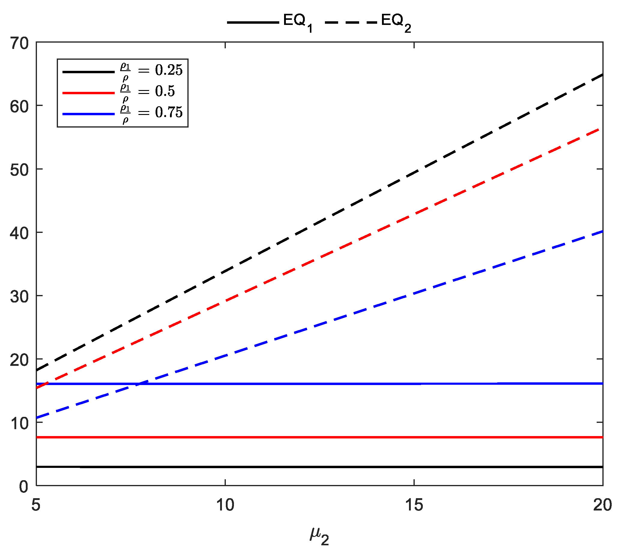
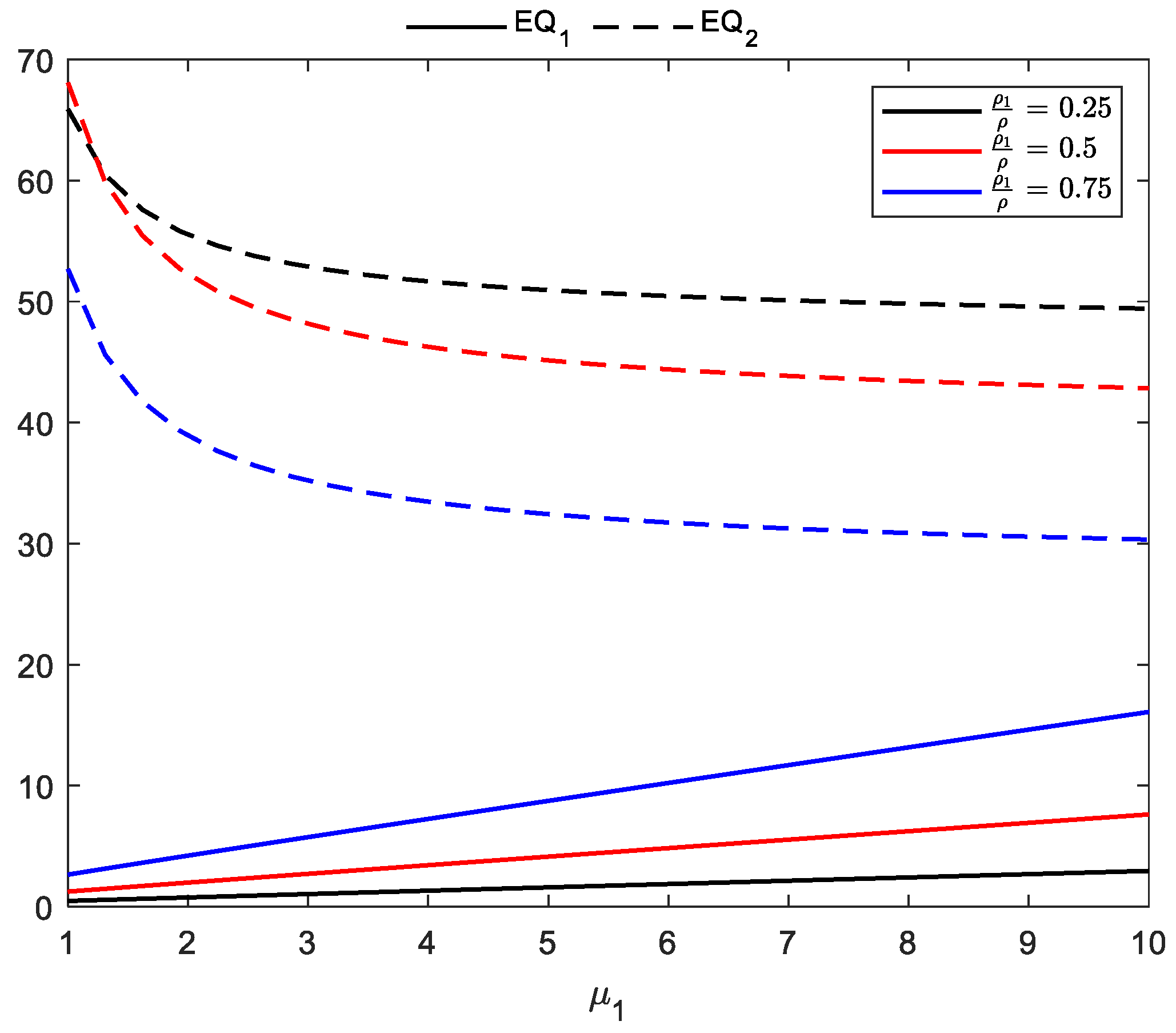
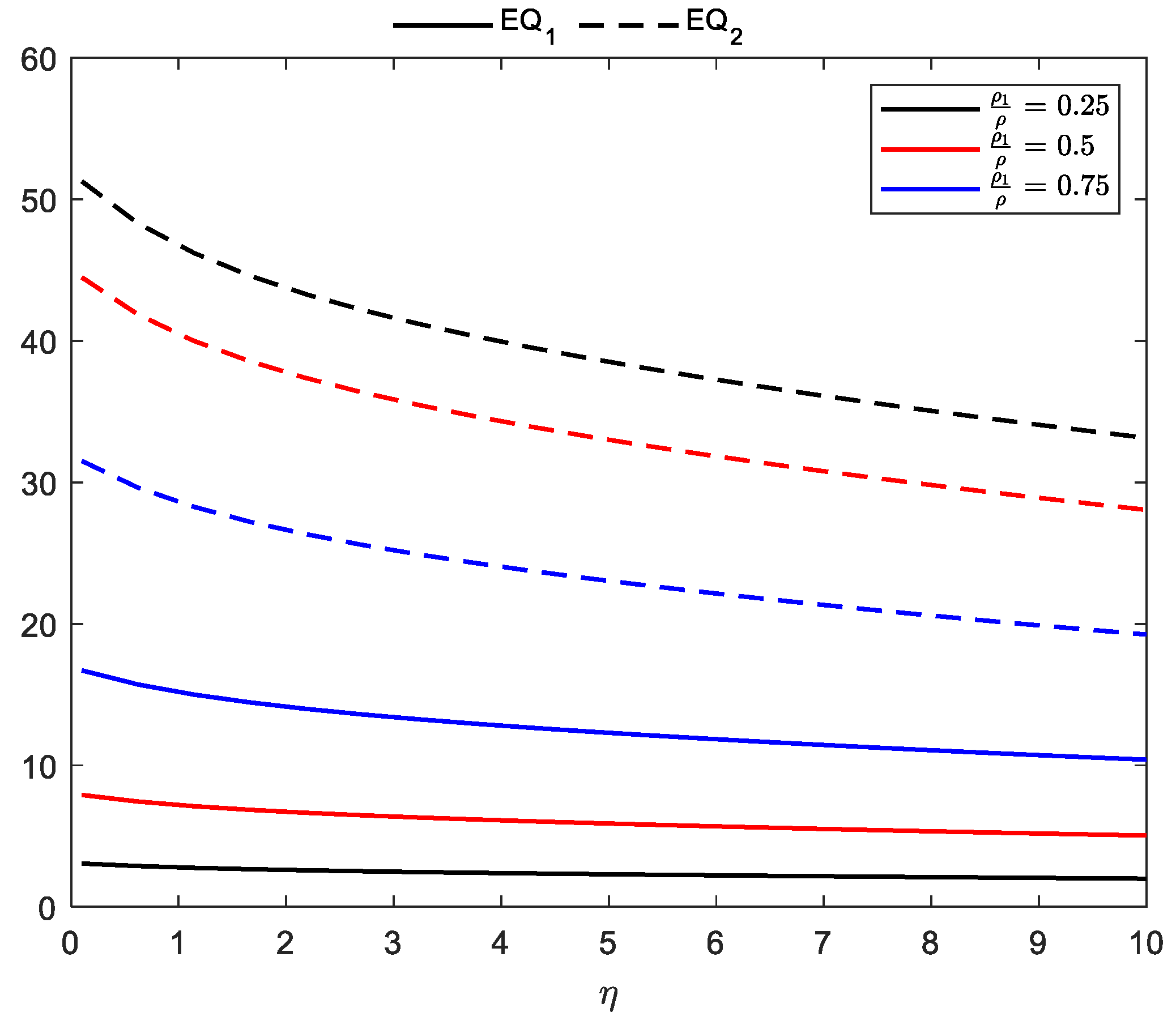
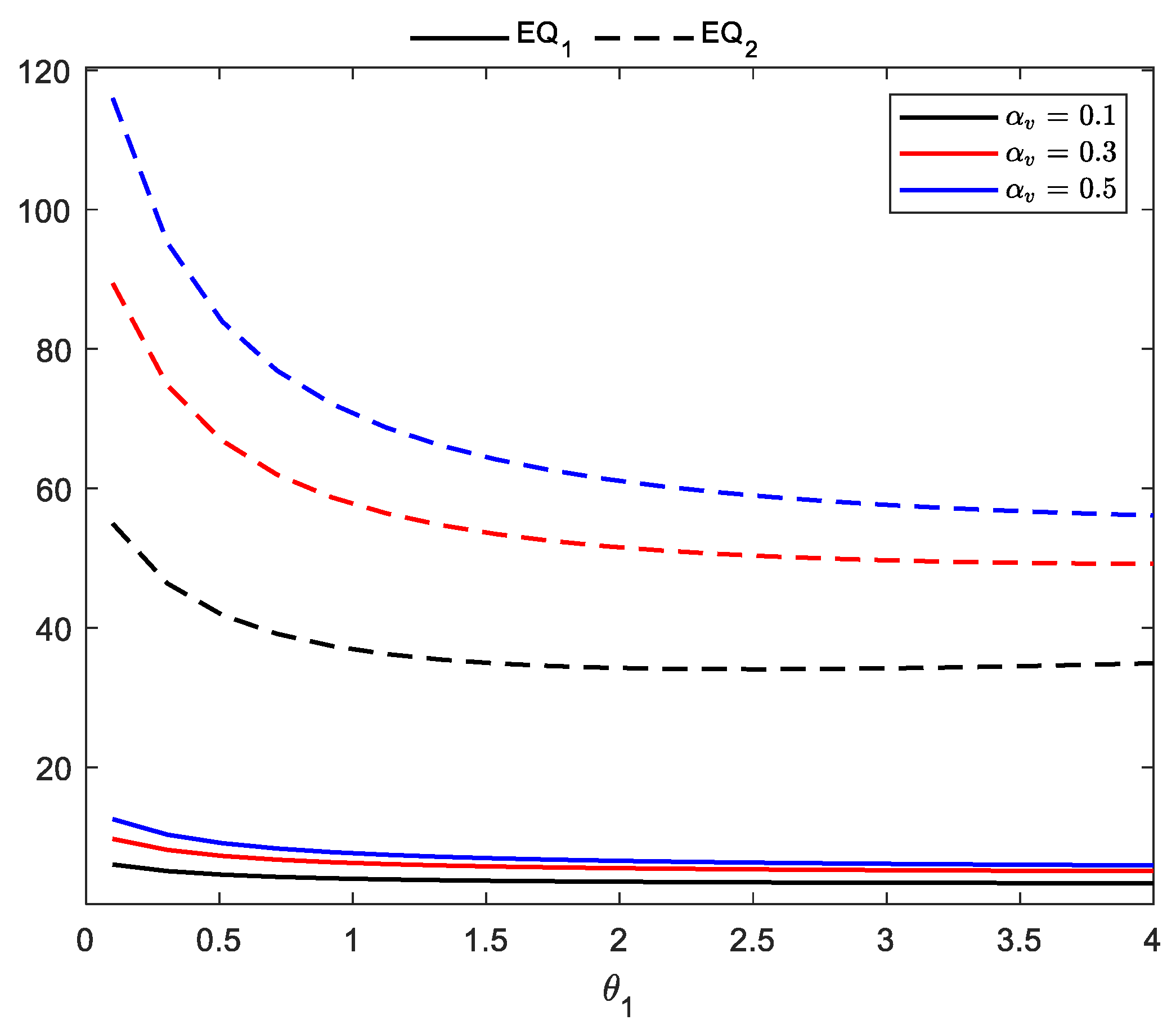
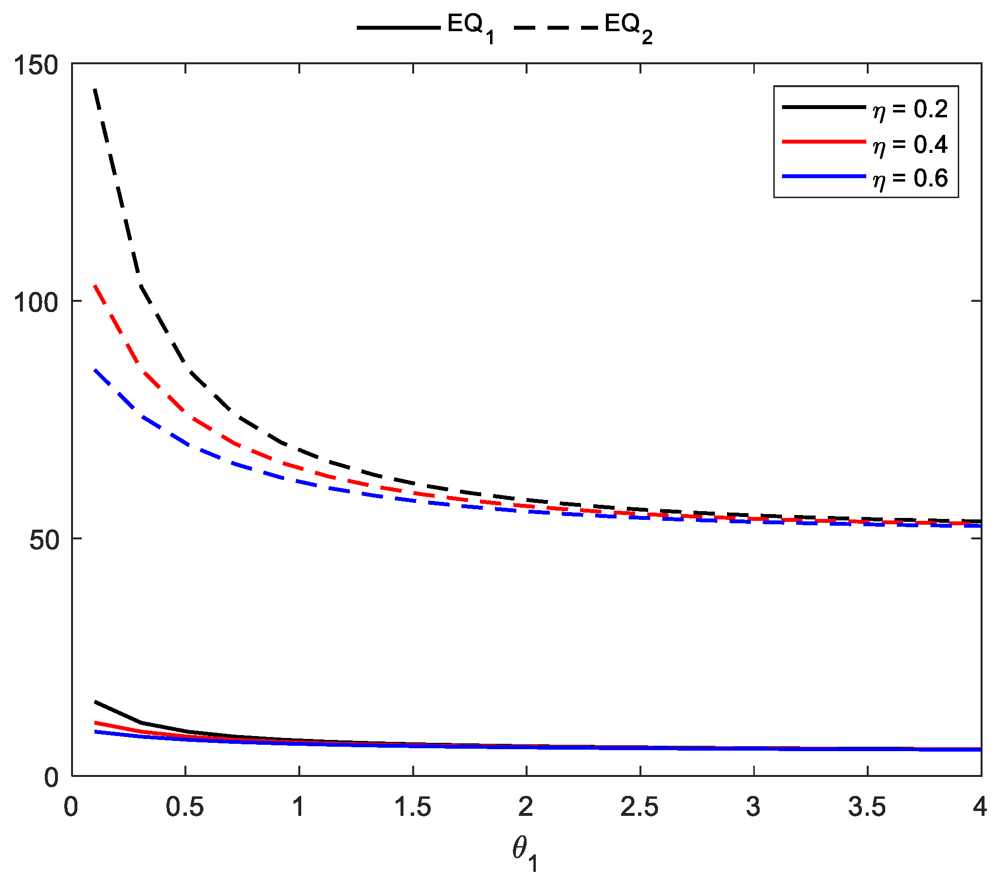
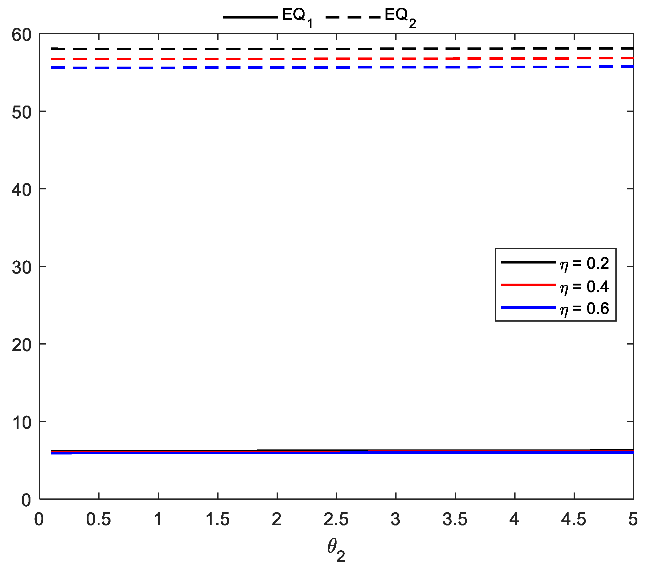
5.1. Effect of System Parameters on the Mean Length of Each Class of Customers
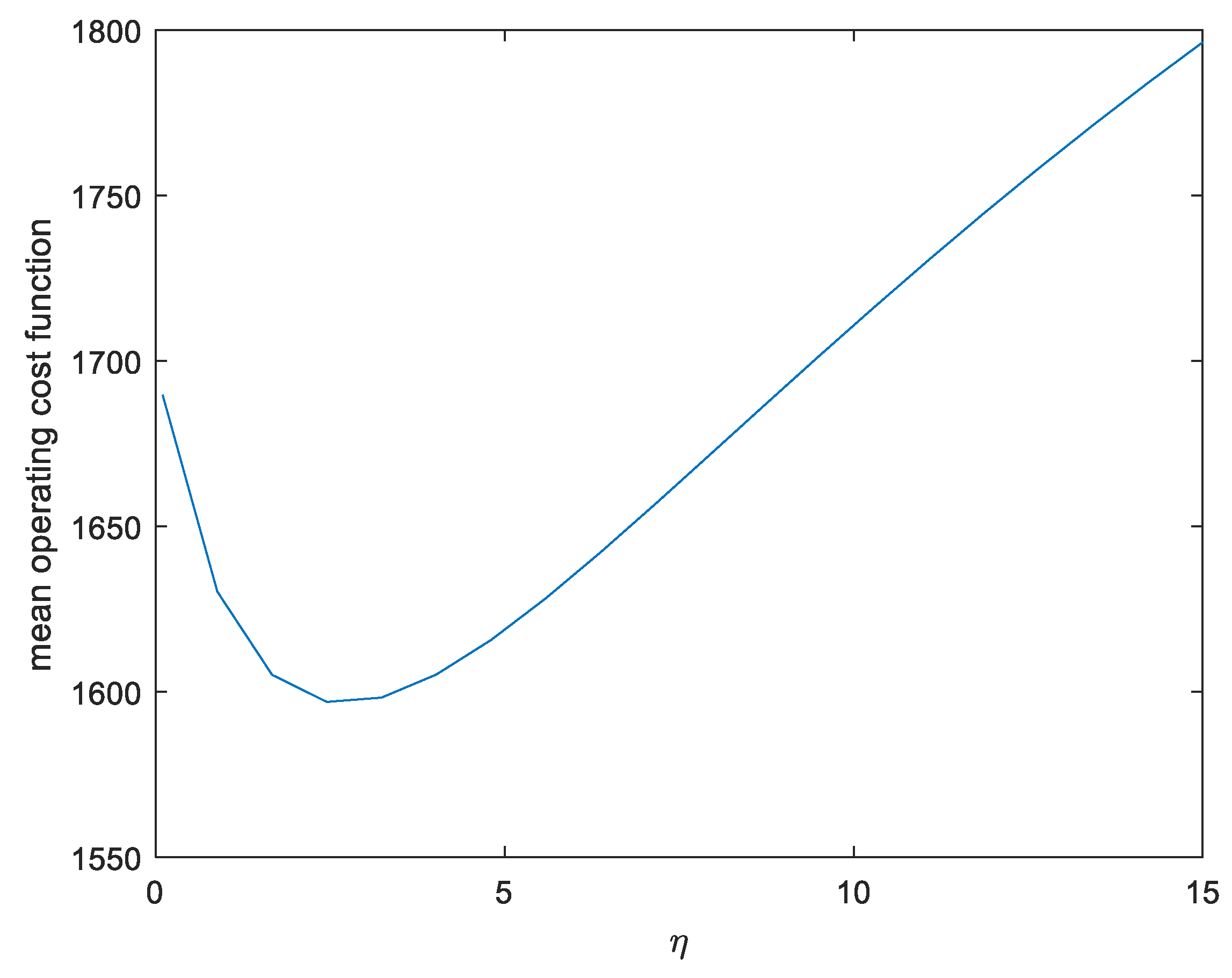
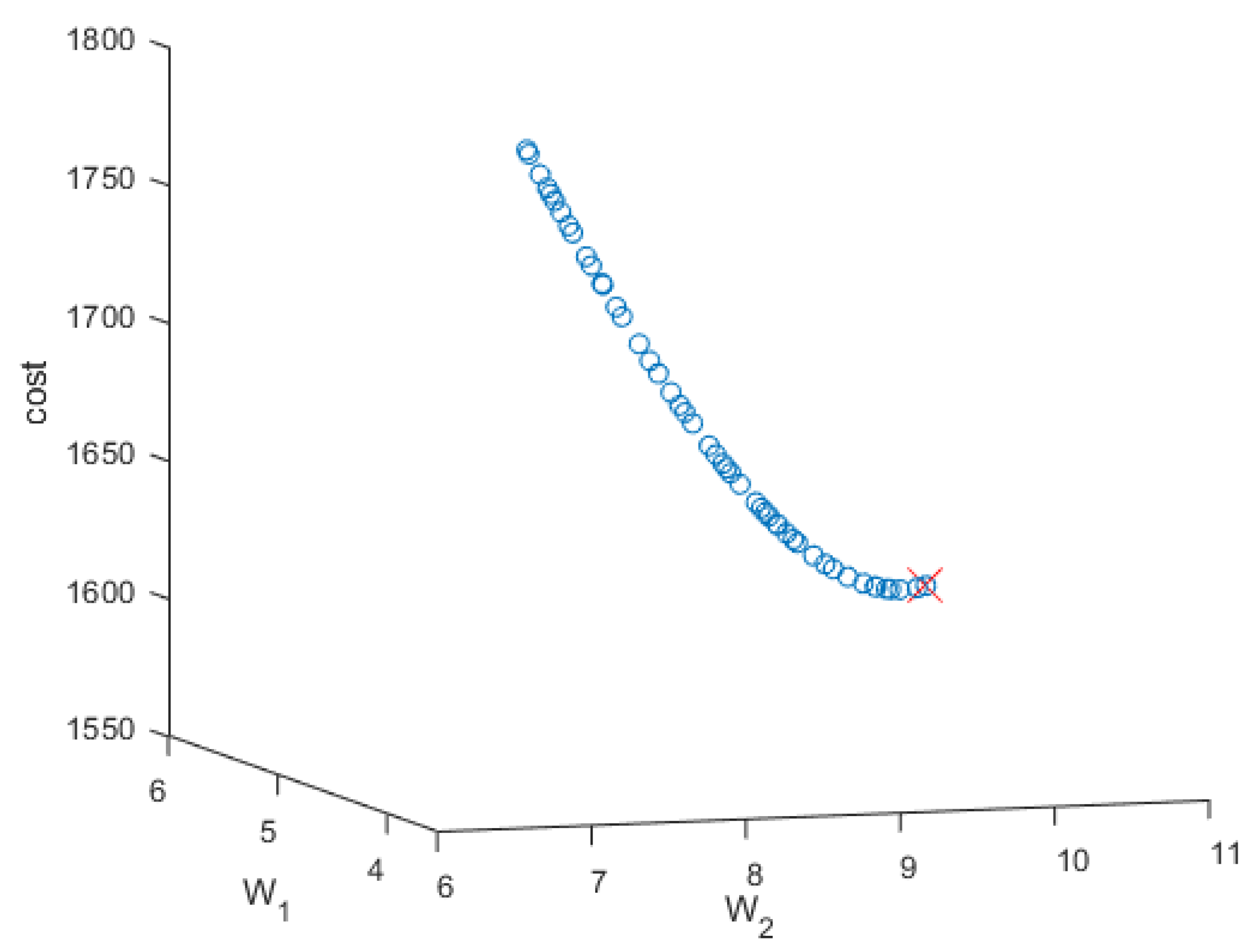
5.2. Cost Optimization
5.3. Waiting Time and Cost Analysis
6. Conclusions Remarks
Author Contributions
Funding
Data Availability Statement
Conflicts of Interest
Appendix A
Appendix B
References
- Tian, N.; Zhang, Z.G. Vacation Queueing Models: Theory and Applications; Springer: Boston, MA, USA, 2006. [Google Scholar]
- Ke, J.C.; Wu, C.H.; Zhang, Z.G. Recent developments in vacation queueing models: A short survey. Int. J. Oper. Res. 2010, 7, 3–8. [Google Scholar]
- Servi, L.D.; Finn, S.G. M/M/1 queues with working vacations (M/M/1/WV). Perform. Eval. 2002, 50, 41–52. [Google Scholar] [CrossRef]
- Tian, N.; Li, J.; Zhang, G. Matrix analysis method and working vacation queueing survey. Int. J. Manag. Sci. 2009, 20, 603–633. [Google Scholar]
- Choudhury, G.; Kalita, C.R. An M/G/1 queue with two types of general heterogeneous service and optional repeated service subject to server’s breakdown and delayed repair. Qual. Technol. Quant. Manag. 2018, 15, 622–654. [Google Scholar] [CrossRef]
- Varalakshmi, M.; Chandrasekaran, V.M.; Saravanarajan, M.C. A single server queue with immediate feedback, working vacation and server breakdown. Int. J. Eng. Technol. 2018, 7, 476–479. [Google Scholar]
- Vijayashree, K.V.; Anjuka, A. Stationary analysis of a fluid queue driven by an M/M/1 queue with working vacation. Qual. Technol. Quant. Manag. 2018, 15, 187–208. [Google Scholar] [CrossRef]
- Kempa, W.M.; Kobielnik, M. Transient solution for the queue-size distribution in a finite-buffer model with general independent input stream and single working vacation policy. Appl. Math. Model. 2018, 59, 614–628. [Google Scholar] [CrossRef]
- Suranga Sampath, M.I.G.; Liu, J. Impact of customers’ impatience on an M/M/1 queueing system subject to differentiated vacations with a waiting server. Qual. Technol. Quant. Manag. 2020, 17, 125–148. [Google Scholar] [CrossRef]
- Shekhar, C.; Varshney, S.; Kumar, A. Matrix-geometric solution of multi-server queueing systems with Bernoulli scheduled modified vacation and retention of reneged customers: A meta-heuristic approach. Qual. Technol. Quant. Manag. 2021, 18, 39–66. [Google Scholar] [CrossRef]
- Bouchentouf, A.A.; Guendouzi, A.; Meriem, H.; Shakir, M. Analysis of a single server queue in a multi-phase random environment with working vacations and customers’ impatience. Oper. Res. Decis. 2022, 32, 16–33. [Google Scholar] [CrossRef]
- Bouchentouf, A.A.; Yahiaoui, L.; Kadi, M.; Majid, S. Impatient customers in Markovian queue with Bernoulli feedback and waiting server under variant working vacation policy. Oper. Res. Decis. 2020, 30, 5–28. [Google Scholar] [CrossRef]
- Vadivukarasi, M.; Kalidass, K. Discussion on the transient behavior of single server Markovian multiple variant vacation queues. Oper. Res. Decis. 2021, 31, 123–146. [Google Scholar] [CrossRef]
- Li, J.; Tian, N. The M/M/1 queue with working vacations and vacation interruptions. J. Syst. Sci. Syst. Eng. 2007, 16, 121–127. [Google Scholar] [CrossRef]
- Lee, D.H. Equilibrium balking strategies in Markovian queues with a single working vacation and vacation interruption. Qual. Technol. Quant. Manag. 2019, 16, 355–376. [Google Scholar] [CrossRef]
- Bouchentouf, A.A.; Guendouzi, A.; Majid, S. On impatience in Markovian M/M/1/N/DWV queue with vacation interruption. Croat. Oper. Res. Rev. 2020, 11, 1–37. [Google Scholar] [CrossRef]
- Shekhar, C.; Varshney, S.; Kumar, A. Optimal and sensitivity analysis of vacation queueing system with F-policy and vacation interruption. Arab. J. Sci. Eng. 2020, 45, 7091–7107. [Google Scholar] [CrossRef]
- Vijayashree, K.V.; Ambika, K. An M/M/1 queue subject to differentiated vacation with partial interruption and customer impatience. Qual. Technol. Quant. Manag. 2021, 18, 657–682. [Google Scholar]
- Choudhury, G.; Deka, M. A batch arrival unreliable server delaying repair queue with two phases of service and Bernoulli vacation under multiple vacation policy. Qual. Technol. Quant. Manag. 2018, 15, 157–186. [Google Scholar] [CrossRef]
- Jiang, T.; Xin, B. Computational analysis of the queue with working breakdowns and delaying repair under a Bernoulli-schedule-controlled policy. Commun. Stat. Theory Methods 2019, 48, 926–941. [Google Scholar] [CrossRef]
- Yang, D.Y.; Cho, Y.C. Analysis of the N-policy GI/M/1/K queueing systems with working breakdowns and repairs. Comput. J. 2019, 62, 130–143. [Google Scholar] [CrossRef]
- Zhang, Y.; Wang, J. Strategic joining and information disclosing in Markovian queues with an unreliable server and working vacations. Qual. Technol. Quant. Manag. 2021, 18, 298–325. [Google Scholar] [CrossRef]
- Brandwajn, A.; Begin, T. Multi-server preemptive priority queue with general arrivals and service times. Perform. Eval. 2017, 115, 150–164. [Google Scholar] [CrossRef]
- Wang, J.; Cui, S.; Wang, Z. Equilibrium strategies in M/M/1 priority queues with balking. Prod. Oper. Manag. 2019, 28, 43–62. [Google Scholar] [CrossRef]
- Kim, K. Delay cycle analysis of finite-buffer M/G/1 queues and its application to the analysis of M/G/1 priority queues with finite and infinite buffers. Perform. Eval. 2020, 143, 102133. [Google Scholar] [CrossRef]
- Kim, B.; Kim, J.; Bueker, O. Non-preemptive priority M/M/m queue with servers’ vacations. Comput. Ind. Eng. 2021, 160, 107390. [Google Scholar] [CrossRef]
- Ajewole, O.R.; Mmduakor, C.O.; Adeyefa, E.O.; Okoro, J.O.; Ogunlade, T.O. Preemptive-resume priority queue system with Erlang service distribution. J. Theor. Appl. Inf. Technol. 2021, 99, 1426–1434. [Google Scholar]
- Gao, S.; Zhang, J.; Wang, X. Analysis of a retrial queue with two-type breakdowns and delayed repairs. IEEE Access 2020, 8, 172428–172442. [Google Scholar] [CrossRef]
- Bonyadi, M.R.; Michalewicz, Z. Particle swarm optimization for single objective continuous space problems: A review. Evol. Comput. 2017, 25, 1–54. [Google Scholar] [CrossRef] [PubMed]
- Goodarzi, A.H.; Diabat, E.; Jabbarzadeh, A.; Paquet, M. An M/M/c queue model for vehicle routing problem in multi-door cross-docking environments. Comput. Oper. Res. 2022, 138, 105513. [Google Scholar] [CrossRef]
- Hajipour, V.; Farahani, R.Z.; Fattahi, P. Bi-objective vibration damping optimization for congested location-pricing problem. Comput. Oper. Res. 2016, 70, 87–100. [Google Scholar] [CrossRef]
- Wu, C.H.; Yang, D.Y. Bi-objective optimization of a queueing model with two-phase heterogeneous service. Comput. Oper. Res. 2021, 130, 105230. [Google Scholar] [CrossRef]


| η* | CF | W1 | W2 | η* | CF | W1 | W2 |
|---|---|---|---|---|---|---|---|
| 3.91 | 1604.039 | 5.41 | 10.09 | 5.04 | 1619.256 | 5.13 | 9.57 |
| 2.84 | 1596.738 | 5.72 | 10.65 | 8.78 | 1687.794 | 4.39 | 8.17 |
| 3.18 | 1597.963 | 5.62 | 10.47 | 7.86 | 1670.044 | 4.55 | 8.48 |
| 11.05 | 1730.026 | 4.04 | 7.51 | 13.36 | 1770.167 | 3.73 | 6.94 |
| 2.69 | 1596.596 | 5.76 | 10.74 | 12.84 | 1761.468 | 3.80 | 7.06 |
| 3.35 | 1599.039 | 5.57 | 10.37 | 12.25 | 1751.377 | 3.87 | 7.20 |
| 10.82 | 1725.915 | 4.07 | 7.57 | 3.67 | 1601.634 | 5.48 | 10.21 |
| 7.33 | 1660.120 | 4.65 | 8.66 | 13.99 | 1780.379 | 3.66 | 6.80 |
| 9.51 | 1701.557 | 4.27 | 7.95 | 14.89 | 1794.540 | 3.55 | 6.60 |
| 11.57 | 1739.440 | 3.96 | 7.37 | 9.07 | 1693.336 | 4.34 | 8.08 |
| 13.02 | 1764.515 | 3.77 | 7.01 | 6.95 | 1652.857 | 4.72 | 8.80 |
| 3.44 | 1599.638 | 5.54 | 10.33 | 8.37 | 1679.905 | 4.46 | 8.31 |
| 6.36 | 1641.983 | 4.84 | 9.02 | 8.62 | 1684.597 | 4.42 | 8.23 |
| 7.65 | 1666.121 | 4.59 | 8.55 | 5.92 | 1634.116 | 4.94 | 9.19 |
| 11.61 | 1740.085 | 3.96 | 7.36 | 10.19 | 1714.271 | 4.16 | 7.75 |
| 5.71 | 1630.279 | 4.98 | 9.28 | 13.66 | 1774.966 | 3.70 | 6.87 |
| 5.96 | 1634.651 | 4.93 | 9.18 | 7.44 | 1662.199 | 4.63 | 8.62 |
| 4.25 | 1608.010 | 5.33 | 9.92 | 6.25 | 1639.998 | 4.87 | 9.06 |
| 5.53 | 1627.281 | 5.02 | 9.36 | 12.04 | 1747.684 | 3.90 | 7.25 |
| 13.83 | 1777.805 | 3.67 | 6.83 | 5.43 | 1625.650 | 5.04 | 9.40 |
| 14.34 | 1786.005 | 3.61 | 6.72 | 7.22 | 1657.917 | 4.67 | 8.70 |
| 6.51 | 1644.585 | 4.81 | 8.97 | 4.58 | 1612.400 | 5.24 | 9.77 |
| 3.65 | 1601.410 | 5.48 | 10.22 | 9.80 | 1706.97 | 4.22 | 7.86 |
| 4.76 | 1615.047 | 5.20 | 9.69 | 6.16 | 1638.26 | 4.89 | 9.10 |
Disclaimer/Publisher’s Note: The statements, opinions and data contained in all publications are solely those of the individual author(s) and contributor(s) and not of MDPI and/or the editor(s). MDPI and/or the editor(s) disclaim responsibility for any injury to people or property resulting from any ideas, methods, instructions or products referred to in the content. |
© 2023 by the authors. Licensee MDPI, Basel, Switzerland. This article is an open access article distributed under the terms and conditions of the Creative Commons Attribution (CC BY) license (https://creativecommons.org/licenses/by/4.0/).
Share and Cite
Liu, T.-H.; Hsu, H.-Y.; Ke, J.-C.; Chang, F.-M. Preemptive Priority Markovian Queue Subject to Server Breakdown with Imperfect Coverage and Working Vacation Interruption. Computation 2023, 11, 89. https://doi.org/10.3390/computation11050089
Liu T-H, Hsu H-Y, Ke J-C, Chang F-M. Preemptive Priority Markovian Queue Subject to Server Breakdown with Imperfect Coverage and Working Vacation Interruption. Computation. 2023; 11(5):89. https://doi.org/10.3390/computation11050089
Chicago/Turabian StyleLiu, Tzu-Hsin, He-Yao Hsu, Jau-Chuan Ke, and Fu-Min Chang. 2023. "Preemptive Priority Markovian Queue Subject to Server Breakdown with Imperfect Coverage and Working Vacation Interruption" Computation 11, no. 5: 89. https://doi.org/10.3390/computation11050089
APA StyleLiu, T.-H., Hsu, H.-Y., Ke, J.-C., & Chang, F.-M. (2023). Preemptive Priority Markovian Queue Subject to Server Breakdown with Imperfect Coverage and Working Vacation Interruption. Computation, 11(5), 89. https://doi.org/10.3390/computation11050089