Article

Modeling and Forecasting of nanoFeCu Treated Sewage Quality Using Recurrent Neural Network (RNN)

1
Centre for Water Research, Faculty of Engineering and the Built Environment, SEGi University, Petaling Jaya 47810, Malaysia
2
Department of Electrical and Electronic Engineering, Guangdong Technology College, Zhaoqing 526100, China
3
Faculty of Arts and Science, International University of Malaya-Wales, Kuala Lumpur 50480, Malaysia
*
Author to whom correspondence should be addressed.
Computation 2023, 11(2), 39; https://doi.org/10.3390/computation11020039
Submission received: 6 January 2023 / Revised: 30 January 2023 / Accepted: 12 February 2023 / Published: 17 February 2023
(This article belongs to the Special Issue Intelligent Computing, Modeling and its Applications)

Abstract

:
Rapid industrialization and population growth cause severe water pollution and increased water demand. The use of FeCu nanoparticles (nanoFeCu) in treating sewage has been proven to be a space-efficient method. The objective of this work is to develop a recurrent neural network (RNN) model to estimate the performance of immobilized nanoFeCu in sewage treatment, thereby easing the monitoring and forecasting of sewage quality. In this work, sewage data was collected from a local sewage treatment plant. pH, nitrate, nitrite, and ammonia were used as the inputs. One-to-one and three-to-three RNN architectures were developed, optimized, and analyzed. The result showed that the one-to-one model predicted all four inputs with good accuracy, where R2 was found within a range of 0.87 to 0.98. However, the stability of the one-to-one model was not as good as the three-to-three model, as the inputs were chemically and statistically correlated in the later model. The best three-to-three model was developed by a single layer with 10 neurons and an average R2 of 0.91. In conclusion, this research provides data support for designing the neural network prediction model for sewage and provides positive significance for the exploration of smart sewage treatment plants.

1. Introduction

Water is a crucial resource for life. Population growth, expansion of irrigated areas, and industrial development increase the global demand for freshwater supply. The global demand for freshwater supplies has increased by more than 600% since the 1960s [1]. Consequently, freshwater shortages have become a threat to sustainable human development [2]. It is prevalent in developing countries because of the poor enforcement of environmental laws and the low awareness of freshwater protection. Water pollution exacerbates the shortage issue. The major causes of water pollution include chemical spills [3], illegal industrial wastewater discharge [4], rural aquaculture wastewater [5], and domestic sewage pollution [6].
Studies showed that sewage polluted the world’s coastlines. Cascade et al. [7] used a geospatial model to measure and map the nitrogen (N) and pathogen-fecal indicator organisms (FIO) found in human sewage in approximately 135,000 watersheds worldwide. The results show that 63% of the nitrogen in coastal waters, which was equivalent to 3.9 Tg N, comes from sewage systems. It affects the safety of seafood, and human pathogens in seafood can lead to outbreaks of foodborne disease [8]. Eventually, it would be a threat to biodiversity and ecosystem health. Efforts have been made by government bodies and researchers to overcome the water pollution issue, especially for sewage treatment. Generally, the sewage treatment process is classified into three stages (primary, secondary, and tertiary treatment) controlled by a combination of physical, chemical, and biological processes. The primary treatment mostly adopts physical methods to treat larger suspended solids and sand in sewage through grid retention, filtration, and sedimentation. This treatment technology is relatively mature. Secondary treatment typically involves biological treatment to remove dissolved and suspended biological matter, such as the activated sludge process (ASP). It is worth noting that the effluent quality of the secondary treatment was unstable due to the microbe’s sensitivity to changes in pH, dissolved oxygen, pollutant concentration, and temperature [9]. Tertiary treatment processes include physical-chemical treatment such as coagulation, flocculation, sedimentation, and filtration, as well as advanced oxidation processes, for instance, photocatalytic oxidation and electrochemical oxidation. Usually, tertiary treatment processes have the advantage of high treatment efficiency and reliable effluent quality, but the process is expensive and possibly causes secondary pollution, such as the degradation of photocatalysts and electrodes [10].
Thus, it is important to create cross-disciplinary synergies to develop innovative technology for sewage treatment to address space and cost-effectiveness issues [11]. Lately, Chan et al. [12] found that FeCu nanoparticles could be used for ammonia removal via the oxidation process. The results demonstrated that the immobilized FeCu nanoparticles exhibited good ammonia removal performance when handling 10–100 ppm of ammonia solutions. The reusability study revealed that the immobilized FeCu could be reused at least three times without deterioration [13]. Meanwhile, the pilot-scale studies also revealed the full potential of immobilized FeCu for sewage treatment [14]. Recently, with the development and availability of computing power and big data, artificial neural networks (ANN) have been successfully applied in many fields, especially sequential prediction, such as rainfall-runoff [15] and weather and hydrological time sequence prediction [16]. In water treatment plants, sensors are used for measuring water level, flowrate, and water quality [17]. This generated a pool of time series data that can be used to monitor treatment efficiency. It is noteworthy that the acquired data are related in complex and nonlinear ways [18]. It is impractical to manually compute and analyze the data. Hence, it is essential to incorporate machine learning into water research.
Table 1 summarizes recent research on the use of machine learning to model and estimate water quality. Wu [19] combined the auto-regressive integrated moving average (ARIMA) and clustering models to improve the poor predictive performance of the traditional time-series ARIMA model for data with random characteristics. Tan [20] proposes a hybrid model for water quality prediction that combines the respective advantages of the convolutional neural network (CNN) model and the long short-term memory (LSTM) model. After the feature extraction of the CNN layer, the original data will get a new sequence with more vital feature ability than the original sequence. Compared with the conventional LSTM model, its mean absolute error was optimized by 11.63%. Li [21] uses several models, including back propagation neural networks (BPNN), radial basis function neural networks (RBFNN), and support vector machines (SVM), to simulate and predict water quality parameters. The results showed that the SVM achieved the best prediction effect, with an accuracy of 99% for both published and measured data.
The ANNs simulate the functions of the human brain [27], in which a large number of widely interconnected neurons form a network to conduct continuous learning, summarize past experience, and store the acquired knowledge. This information is then used for future forecasting [28]. During the training process, the network continuously adjusts its weights to minimize errors. If the network makes a poor prediction, the connection weights in the network will be adjusted in order to increase accuracy. Thus, the network is less likely to make the same mistake during the next iteration [29,30]. ANN is a general approximator that extracts the nonlinear relationships and interactions from different data features and solves large-scale problems by identifying the relationships in a given pattern [31], such as time series forecasting, pattern recognition, nonlinear modeling, classification, and control [32].
The recurrent neural network (RNN) is a versatile and easily assembled ANN [33]. The conventional ANN architecture is composed of an input layer, multiple hidden layers, and an output layer. Each layer consists of numerous interconnected neurons [34]. A neuron is a non-linear algebraic function [35]. When the signal is applied to the input of the neuron, its weights are modified [36]. Contrary to other neural network architectures, RNN uses state variables to store previous information. The output is then computed based on the current and previous states. Therefore, the RNN is widely used in the applications of time series, such as natural language processing, speech recognition, and machine translation [37]. However, it is noted that conventional RNNs usually do not perform well for long sequences due to gradient disappearance and gradient exploding [38]. These issues can be effectively addressed by optimizing the activation function or changing the network architecture [39].
The analysis based on experiments showed that the changes in the water quality parameters are not entirely random. Not only are there correlations among the water quality parameters, but the current statistical moments of the parameters are also closely related to the past moments, and these changes have certain asymptotic characteristics [40]. This characteristic makes it advantageous to use RNN for modeling water quality parameters. It is noted that the selection of appropriate input variables is an important step in the development of deep learning models. The work aims to develop an RNN model to predict the performance of immobilized nanoFeCu for sewage treatment with a focus on nitrogen compounds, including ammonia, nitrate, and nitrite. In this work, the water quality parameter data is obtained from a local sewage treatment plant. An ANN is designed for predicting the water quality to explore the correlation between the data, improve the prediction accuracy, and finally obtain the prediction results based on different network architectures and parameters. The study’s findings provide an exemplary model for predicting nano-FeCu-treated sewage using an RNN approach, which has not been studied previously. This work would serve as an important reference for the researchers and engineers who are exploring smart sewage treatment and nanotechnology.

2. Methodology

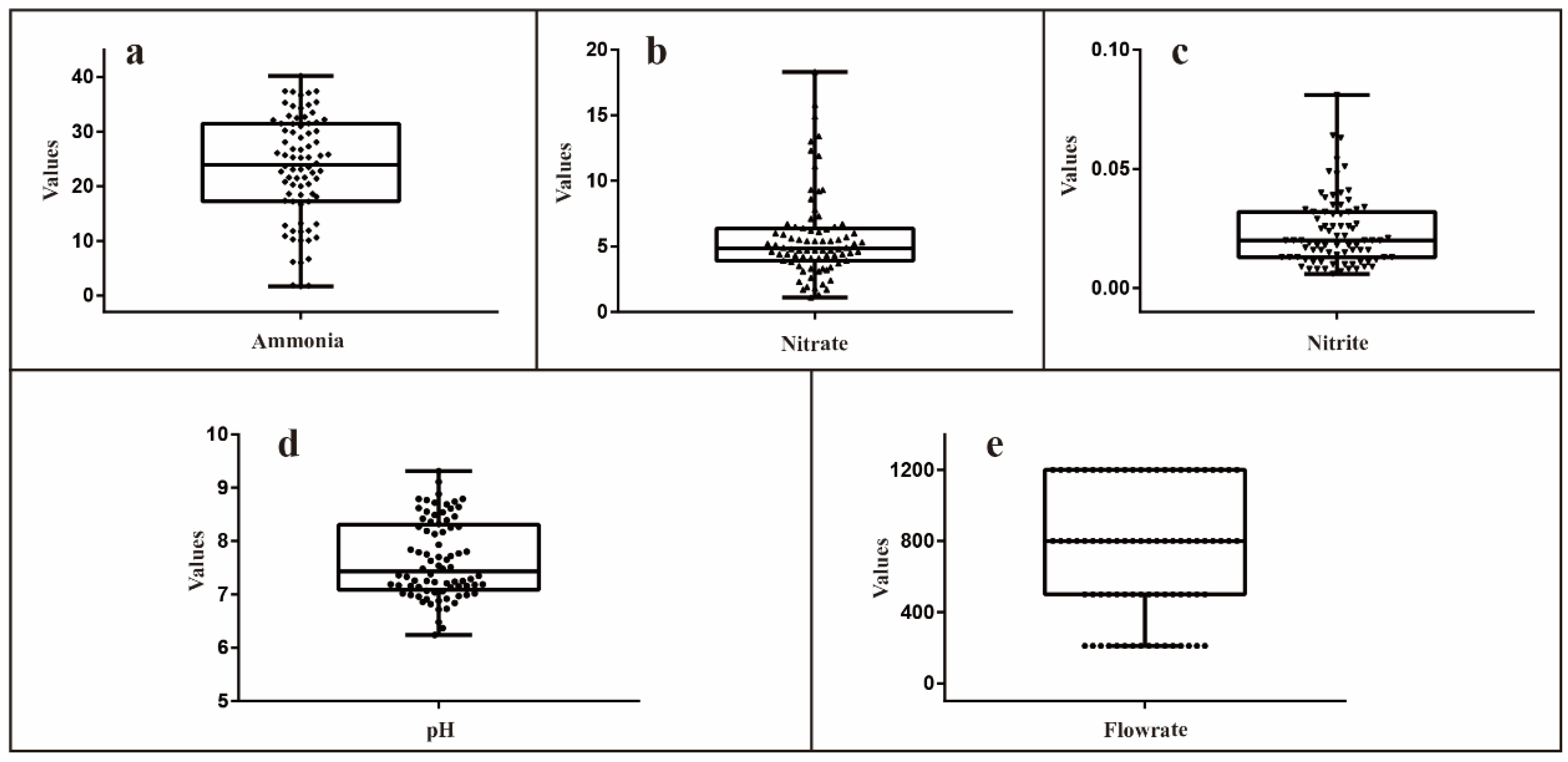
2.1. Data Collection and Processing

The data was collected from a pilot-scale study conducted at a local sewage treatment plant. 100 g of immobilized nanoFeCu was placed in a 50-L reactor and used to treat the sewage for a period of 27 weeks. A total of 84 sets of data were collected for ammonia, nitrate, nitrite, and pH readings at varied flowrates in the range of 210 mL/min to 1200 mL/min, from time t = 0 h to t = 7 h.
The data preprocessing is done by data screening, data cleaning, and data normalization. The purpose of data screening and cleaning is to filter out missing values and address the problem of outliers, which could be due to unpredictable weather during the process of data acquisition. The process of data cleaning to identify outliers in the dataset is performed based on the Pauta criterion [41]. Lastly, the data was normalized using the min-max normalization method, where the data was linearly transformed within the range of 0 to 1 for both inputs and outputs [42]. This is done to ensure that the data is properly fitted to the model. The min-max normalization method is mathematically expressed as Equation (1)
y i = x i min 1 j n { x j } max 1 j n { x j } min 1 j n { x j }
where x i denotes the raw data and y i denotes the normalized value. Xmin and Xmax represent the minimum and maximum data, respectively.
The statistically analyzed data was presented in Table 2 and illustrated using a box-and-whisker plot, as illustrated in Figure 1. The processed data were divided into 10 groups according to the collection time and flowrate. 90% of the data was used for training, and the remaining 10% was used for testing purposes.

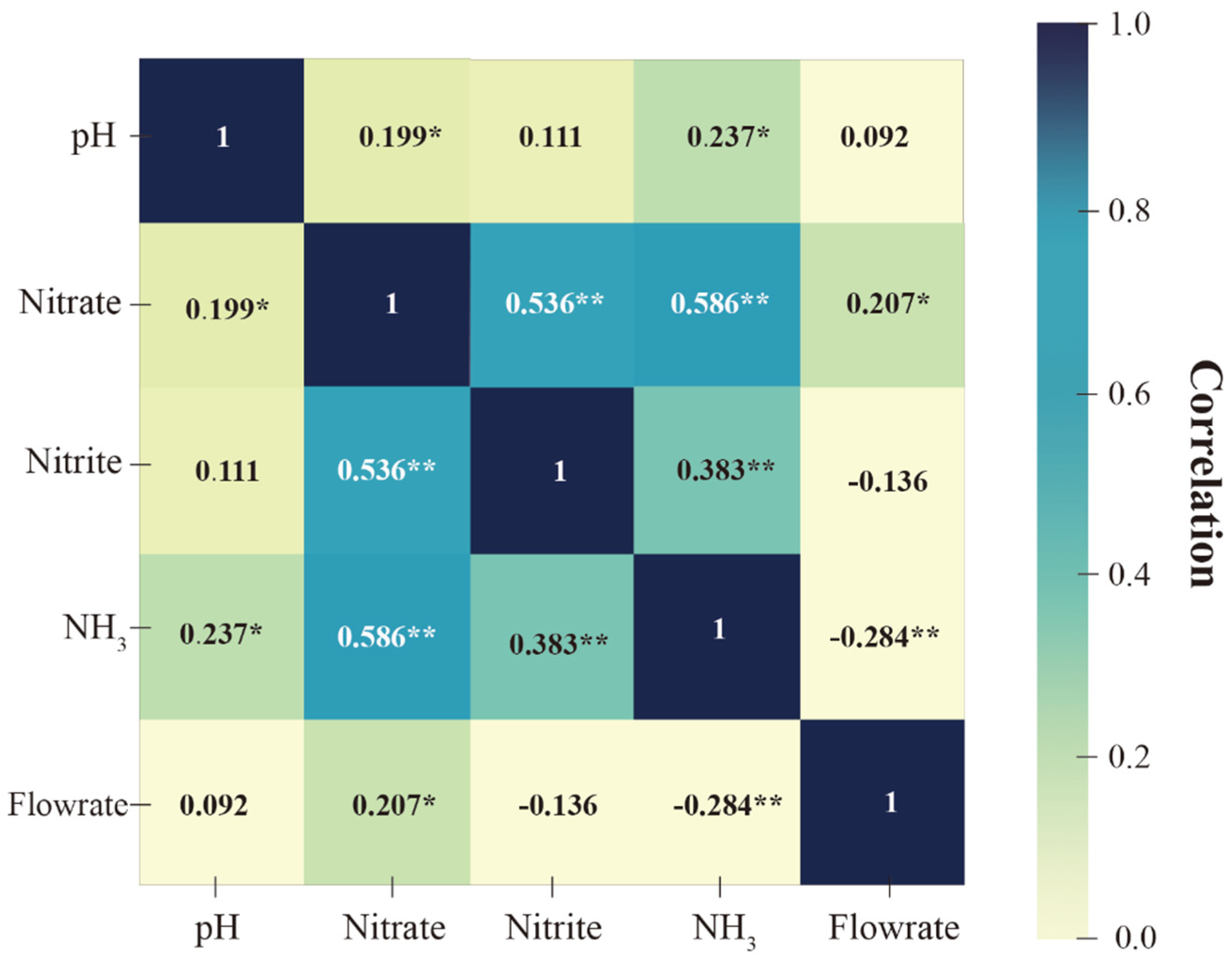
2.2. Pearson Correlation Coefficient

The Pearson correlation coefficient, as presented in Equation (2), was used to identify the relation between the inputs using SPSS 26 software
r = ( x i x ¯ ) ( y i y ¯ ) ( x i x ¯ ) 2 ( y i y ¯ ) 2
r = correlation coefficient
x i = values of the x-variable in a sample
x ¯ = mean of the values of the x-variable
y i = values of the y-variable in a sample
y ¯ = mean of the values of the y-variable

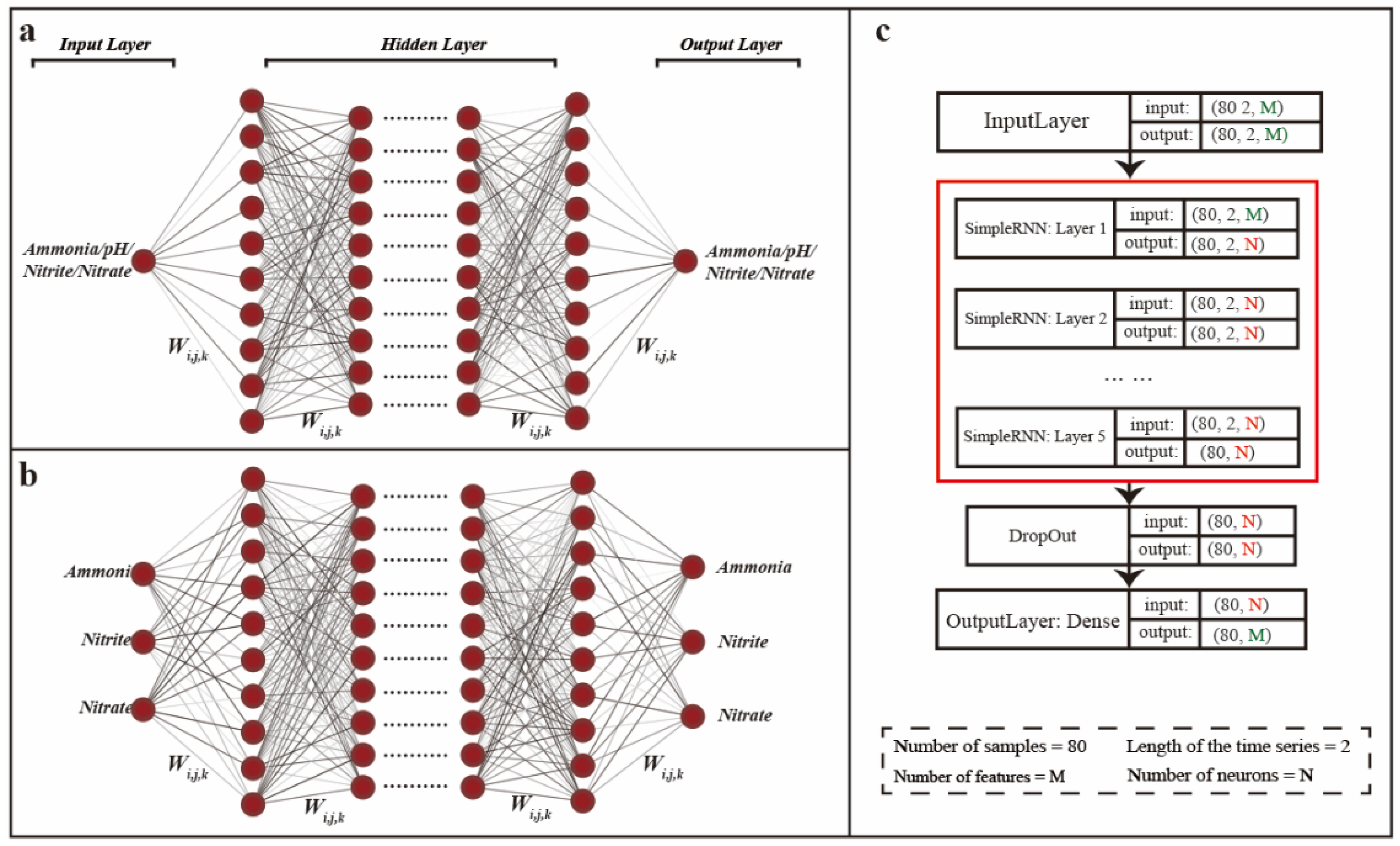
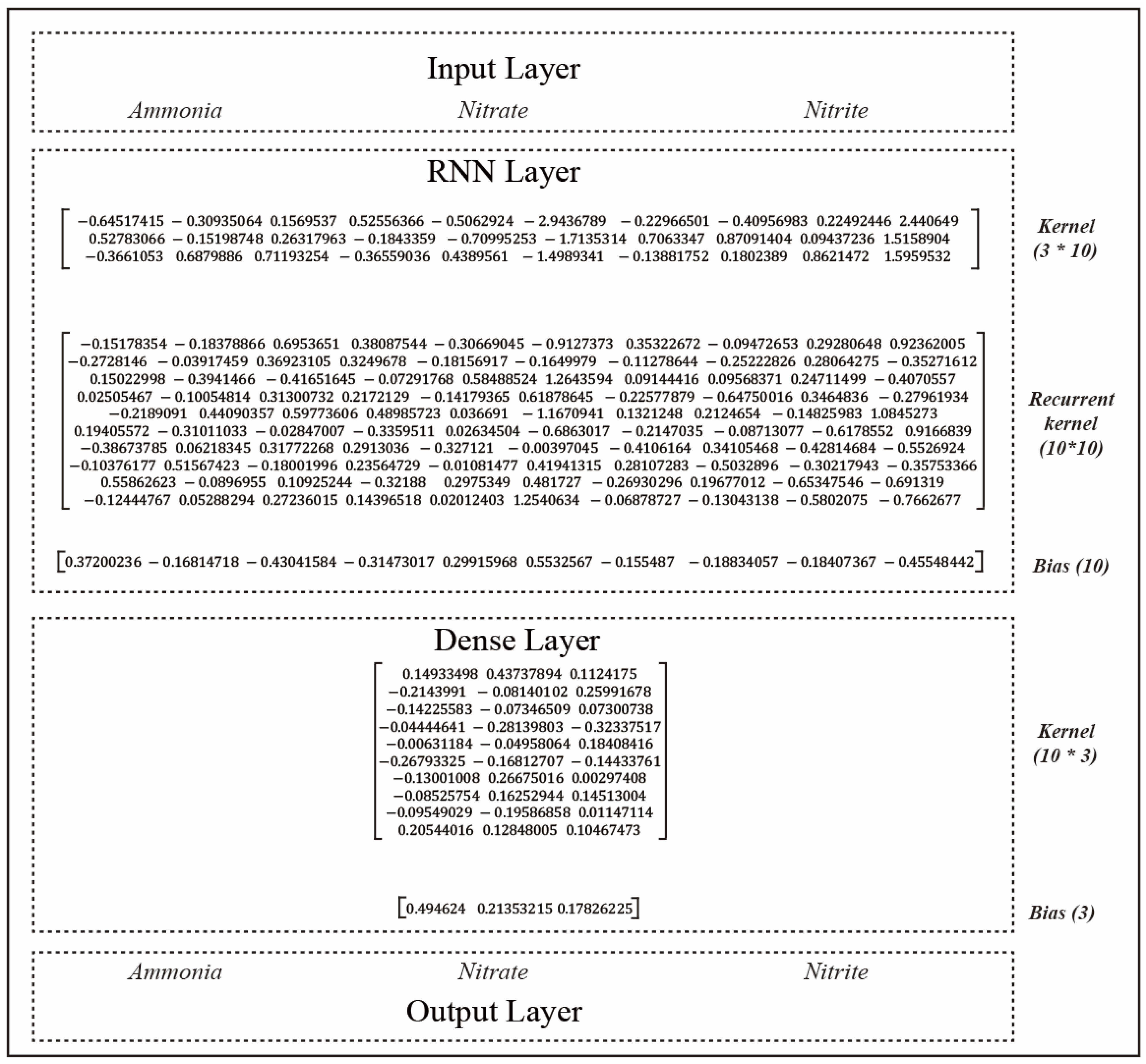
2.3. Model Setup and Implementation

Table 3 shows the RNN architectures adopted in this study, which are ideal to model time series data. pH, ammonia, nitrate, and nitrite at different time intervals were used as the inputs and outputs of the model. In this study, flowrate is the manipulated variable, which affects the performance of immobilized nanoFeCu. The flowrate was not affected by the time; thus, it was not used to develop the model. The number of neurons and hidden layers were manipulated within the range of 10–50 and 1–5, respectively, to increase the model’s performance. The dropout rate was set at 0.09. ReLU was chosen as the activation function as it is faster than Sigmoid and Tanh due to its simple function composition (when x ≤ 0, output = 0, and when x > 0, output = x) [43]. In addition, the non-saturating activation function of ReLU avoids the vanishing gradient. The RNN model is developed using TensorFlow, which is open-source software for deep learning [44]. 1000 iterations were used in this study due to minimum training loss, as illustrated in Figures S1–S5.
Figure 2a,b present the one-to-one and three-to-three RNN architectures. Figure 2c presents the design scheme of the RNN model. In the one-to-one model, one of the inputs, for example pH at t = 1 and 2 h, was used to predict the subsequent output at the following time interval, which was pH at t = 3 h. Meanwhile, three inputs (ammonia, nitrate, and nitrite) at a specific time were used to estimate the subsequent outputs in the three-to-three model. This means that ammonia, nitrate, and nitrite at t = 1 h and 2 h served as the inputs for ammonia, nitrate, and nitrite at t = 3 h.
The accuracy of prediction is measured by the coefficient of determination (R2) as presented in Equation (3)
R 2 = ( i = 1 n ( c t i c ¯ t ) · ( c t i c ¯ p ) ) 2 i = 1 n ( c t i c ¯ t ) 2 · i = 1 n ( c p i c ¯ p ) 2
n denotes the number of data, c t i represents the true value at the ith sample, c p i represents the predicted value for the ith sample, and c ¯ p and c ¯ t represent the average of the predicted results and the real results, respectively.

3. Result and Discussion

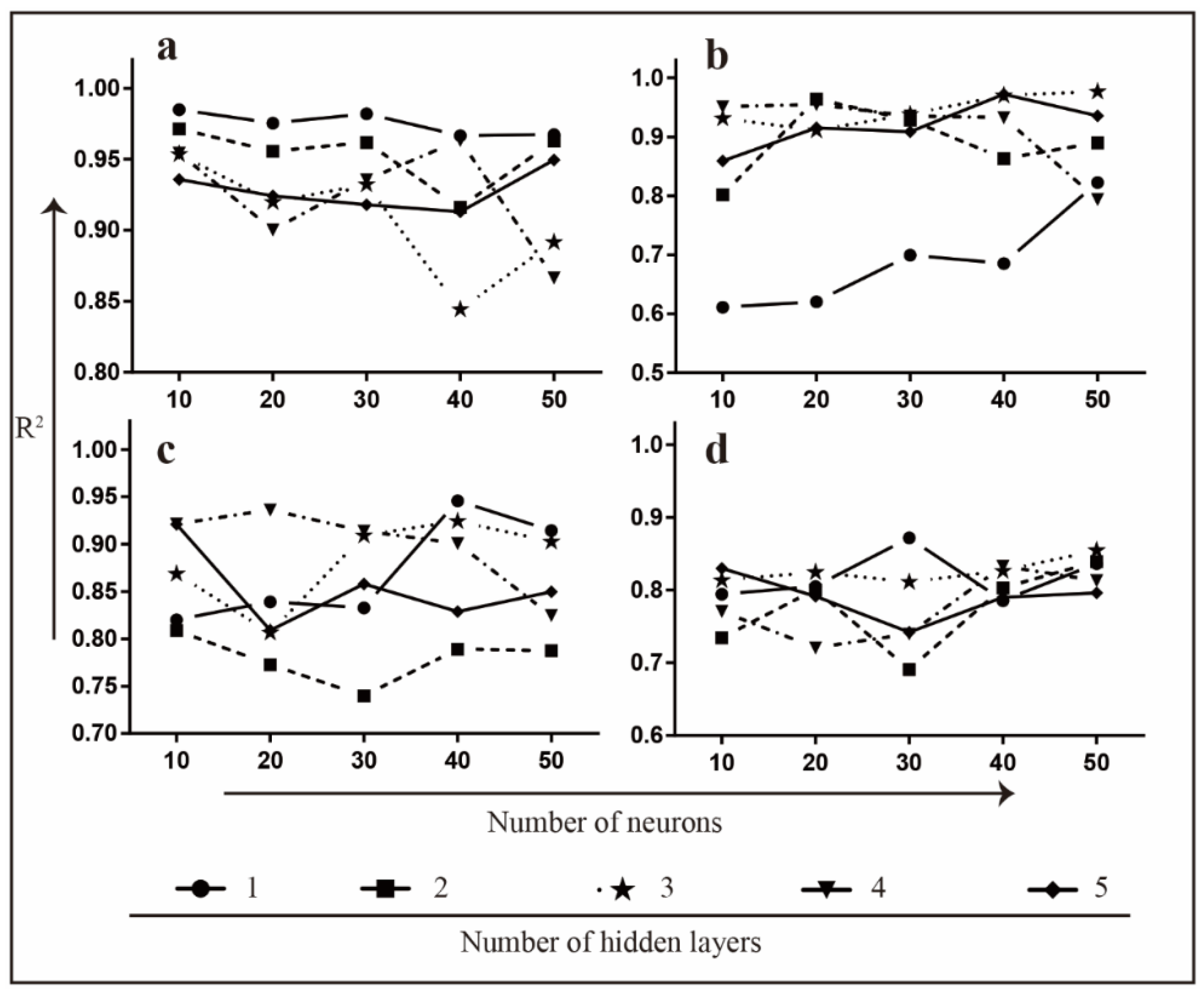
3.1. The Performance of One-to-One Model in Ammonia, Nitrate, Nitrite and pH Prediction

Figure 3 shows the prediction results of the one-to-one model for (a) pH, (b) ammonia, (c) nitrate, and (d) nitrite. In Figure 3a, when the number of hidden layers is 1, the R2 value is almost not affected by the number of neurons. However, as the number of hidden layers increases, the R2 value decreases. It could be clearly observed in the model, which consisted of 3 hidden layers and 40 neurons, where the R2 was equal to 0.844, while the model with a single layer and 40 neurons has a R2 value of 0.966. This could be due to the fact that the change in pH was not significant during the nanoFeCu-triggered ammonia oxidation process, as shown in Table 2, where the SD value of pH is 0.816. This indicates that a single layer is sufficient to develop a good model to predict the pH. A similar trend was observed in the nitrite model, where a small SD value of 0.014 was observed in Table 2, and Figure 3d showed that a single layer was good enough to predict its performance with a high R2 of ~0.8. The best nitrite prediction was found in the model with a single hidden layer, 30 neurons, and an R2 value of 0.872.
A similar approach was used to predict ammonia and nitrate, as shown in Figure 3b,c. In Figure 3b, one hidden layer is insufficient to support the model and achieve good results in predicting the value of ammonia. The increase in the number of neurons improves the performance of the prediction (R2 from 0.611~0.823), which indicates that the model structure of one hidden layer is too simple to extract the features of complex data. When the hidden layers are increased to 2–5 layers, the performance of the model is basically stable, and the R2 of the models is all greater than 0.793. The highest R2 value of 0.9770 was achieved from 3 hidden layers and 50 neurons in the RNN. For nitrate prediction, different variations of hidden layers and neurons can all achieve results with R2 > 0.8, except when the hidden layer is 2 and the neurons >10, as depicted in Figure 3c. A maximum R2 of 0.9456 was found in the RNN model with a single layer and 40 neurons. Comparatively, the R2 of pH and nitrite were higher than ammonia and nitrate, which could be due to the higher SD of ammonia and nitrate, which were 3.247 and 9.731, as tabulated in Table 2.
The result of the existing study is better than the work published by Lei [45], where back propagation neural network (BPNN) and radial basis function neural network (RBFNN) were used to predict pH, ammonia, nitrite, and nitrate. The highest R2 values of pH (R2 = 0.84) and ammonia (R2 = 0.88) were obtained by using RBFNN. Meanwhile, the highest R2 value of 0.96 for nitrate and 0.87 for nitrite were reported for BPNN. In the current study (one-to-one model), the highest R2 values for pH, ammonia, nitrate, and nitrite were 0.985, 0.977, 0.946, and 0.872, respectively. This could be due to the suitability of RNNs to handle time-series data.

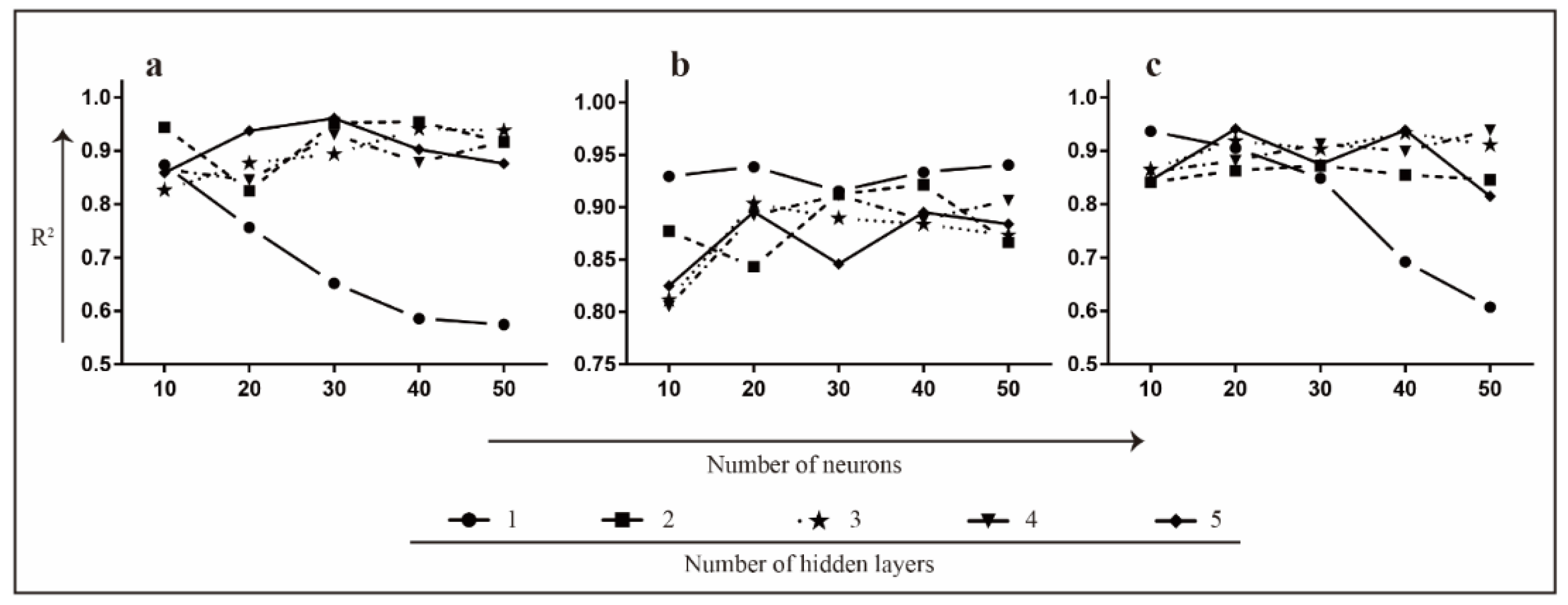
3.2. The Performance of Three-to-Three Model in Ammonia, Nitrate and Nitrite Prediction

A three-to-three model to predict the performance of ammonia, nitrate, and nitrite was developed, and the results are presented in Figure 4. This model was made as there was a close relationship between these three reactants in ammonia oxidation processes [12,13], as indicated in Equations (4)–(10). Nitrate and nitrite are the intermediate products used to oxidize ammonia to nitrogen gas with the aid of nanoFeCu. Fe releases the electrons to facilitate the oxidation process, while Cu assists in the electron transfer [46,47].
In Figure 4, for a single hidden layer, the added neurons decrease the R2 value of the model, especially in Figure 4a,b. This could indicate that the increasing number of neurons leads to the risk of overfitting the model. It is noteworthy that the change in neurons from 10 to 50 did not cause a dramatic change in R2 values when the number of hidden layers was increased from 1 to 5, as shown in Figure 4a,b. This suggests that when the hidden layer is small, even increasing the number of neurons may not lead to better prediction results. The best R2 predictions for ammonia, nitrate, and nitrite were 0.961 with 5 layers and 30 neurons, 0.940 with a single layer and 50 neurons, and 0.941 with 5 layers and 20 neurons, respectively. In addition, the three-to-three model predicted ammonia, nitrate, and nitrite well with an R2 value of > 0.9, except for the results of the single hidden layer.
NH 4 Cl + H 2 O H 3 O + + NH 3 + Cl
2 NH 3 + 4 O 2 NO 2 + NO 3 + 3 H 2 O
Fe 0 2 e + Fe 2 +
NO 3 + 2 e + H 2 O NO 2 + 2 OH
H 2 O + e OH + H ads
2 NO 2 + 4 H ads N 2 + 4 OH
2 NO 2 + 12 H ads 2 NH 4 + + 4 OH

3.3. The Comparison of One-to-One and Three-to-Three Models in Ammonia, Nitrate and Nitrite Estimation

The best RNN architectures of one-to-one and three-to-three models for predicting ammonia, nitrate, and nitrite were identified from Figure 3 and Figure 4. The selection criteria were made based on the R2 values and simplicity of RNN architectures. Based on the average R2 values of three-to-three models, a single hidden layer with 10 neurons was identified as the best RNN architecture, where the R2 average was equal to 0.9132. The R2 values for ammonia, nitrate, and nitrite were 0.8736, 0.9295, and 0.9366, respectively, as presented in Table 4. Compared to the one-to-one model, the R2 values of ammonia, nitrate, and nitrite were much lower, whereas the values were 0.6110, 0.8201, and 0.7943 for the same design of RNN architecture. The high R2 value found in the three-to-three model could be due to the chemical reaction between the three nitrogen compounds, as shown in Equations (4)–(10). This is also proved by the Person correlation coefficient chart, as illustrated in Figure 5, where ammonia, nitrate, and nitrite were significantly correlated at the 0.01 level. The details of the comparison between the one-to-one and three-to-three models are available in the supplementary data, Tables S1 and S2.
The Pearson correlation coefficient chart in Figure 5 showed that the correlation between pH and flowrate is lowest at r = 0.092. This indicates that pH and flowrate are independent parameters. Hence, these two parameters were not considered when developing the three-to-three model. It is notable that there is a weak correlation among pH, ammonia, and nitrate. This is because pH affects the NH 4 + and NH3 equilibrium [48], which eventually affects the formation of nitrate, as shown in Equation (10).
It was observed that the stability of the prediction model is higher in the three-to-three model compared to the one-to-one model, as depicted in Figure 3 and Figure 4. When a one-to-one model was used to predict nitrate, the R2 fluctuated from 0.740 (2 hidden layers and 30 neurons) to 0.946 (1 hidden layer and 40 neurons), as shown in Figure 3c. In Figure 4b, the three-to-three model becomes relatively stable, and R2 ranges from 0.805 (4 hidden layers and 10 neurons) to 0.940 (1 hidden layer and 30 neurons). This demonstrates the improved predictive stability of the model.
The coefficient matrix and bias values for the three-to-three model (single hidden layer and 10 neurons) are shown in Figure 6.

4. Conclusions

In this work, one-to-one and three-to-three RNN models were developed, optimized, and compared to identify the best model to predict and forecast the performance of nanoFeCu in sewage treatment. The R2 values of the one-to-one model for predicting pH, ammonia, nitrate, and nitrate fell within the range of 0.87 to 0.98. However, the overall performance of the model decreases and the results fluctuate when the number of hidden layers and neurons is increased. Comparatively, the stability of the three-to-three model was better as the nitrogen compounds are chemically related in the oxidation process. It is also proved by the Person correlation coefficient, where the nitrogen compounds were significantly correlated at the 0.01 level. Besides, the three-to-three model also improved the overall prediction performance. The best RNN architecture for predicting the nanoFeCu-treated sewage was identified at a single layer with 10 neurons, where an average R2 of 0.91 was recorded. The findings of this study showed that the RNN model developed in this study is suitable for a contact time of up to 7 h. The accuracy of the model could be reduced if the data is collected for >7 h due to the exploding and vanishing gradients problem in time series [49,50]. It is recommended to extend the research by developing the model using other machine learning approaches for a comparative study.

Supplementary Materials

The following supporting information can be downloaded at: https://www.mdpi.com/article/10.3390/computation11020039/s1. Table S1: The results for different numbers of neurons and hidden layers in one-to-one models. Table S2: The results for different numbers of neurons and hidden layers in three-to-three models. Figures S1–S5: The loss values of different neurons and hidden layers for three-to-three models at 1000 iterations.

Author Contributions

D.C.: software, validation, formal analysis, investigation, writing—original draft preparation, visualization. M.C.: conceptualization, methodology, formal analysis, investigation, resources, data curation, writing—original draft preparation, writing—review and editing, supervision, funding acquisition, project administration. S.N.: validation, writing—review and editing. All authors have read and agreed to the published version of the manuscript.

Funding

This research was funded by SEGi University, grant number SEGiIRF/2022-Q1/FoEBEIT/003.

Data Availability Statement

Data are available upon reasonable request.

Acknowledgments

Professional advice and support by the late Chan Chin Wang to this study are greatly appreciated.

Conflicts of Interest

The authors declare no conflict of interest.

References

  1. Piesse, M. Global Water Supply and Demand Trends Point towards Rising Water Insecurity. Analysis and Policy Observatory. 2020. Available online: https://apo.org.au/node/276976 (accessed on 27 February 2020).
  2. Ma, T.; Sun, S.; Fu, G.; Hall, J.W.; Ni, Y.; He, L.; Yi, J.; Zhao, N.; Du, Y.; Pei, T.; et al. Pollution Exacerbates China’s Water Scarcity and Its Regional Inequality. Nat. Commun. 2020, 11, 650. [Google Scholar] [CrossRef] [PubMed] [Green Version]
  3. Jiang, J.; Han, F.; Zheng, Y.; Wang, N.; Yuan, Y. Inverse Uncertainty Characteristics of Pollution Source Identification for River Chemical Spill Incidents by Stochastic Analysis. Front. Environ. Sci. Eng. 2018, 12, 6. [Google Scholar] [CrossRef]
  4. Mukate, S.; Wagh, V.; Panaskar, D.; Jacobs, J.A.; Sawant, A. Development of New Integrated Water Quality Index (IWQI) Model to Evaluate the Drinking Suitability of Water. Ecol. Indic. 2019, 101, 348–354. [Google Scholar] [CrossRef]
  5. Yi, X.; Lin, D.; Li, J.; Zeng, J.; Wang, D.; Yang, F. Ecological Treatment Technology for Agricultural Non-Point Source Pollution in Remote Rural Areas of China. Environ. Sci. Pollut. Res. 2021, 28, 40075–40087. [Google Scholar] [CrossRef]
  6. Nsenga Kumwimba, M.; Meng, F.; Iseyemi, O.; Moore, M.T.; Zhu, B.; Tao, W.; Liang, T.J.; Ilunga, L. Removal of Non-Point Source Pollutants from Domestic Sewage and Agricultural Runoff by Vegetated Drainage Ditches (VDDs): Design, Mechanism, Management Strategies, and Future Directions. Sci. Total Environ. 2018, 639, 742–759. [Google Scholar] [CrossRef]
  7. Tuholske, C.; Halpern, B.S.; Blasco, G.; Villasenor, J.C.; Frazier, M.; Caylor, K. Mapping Global Inputs and Impacts from of Human Sewage in Coastal Ecosystems. PLoS ONE 2021, 16, e0258898. [Google Scholar] [CrossRef]
  8. Littman, R.A.; Fiorenza, E.A.; Wenger, A.S.; Berry, K.L.E.; van de Water, J.A.J.M.; Nguyen, L.; Aung, S.T.; Parker, D.M.; Rader, D.N.; Harvell, C.D.; et al. Coastal Urbanization Influences Human Pathogens and Microdebris Contamination in Seafood. Sci. Total Environ. 2020, 736, 139081. [Google Scholar] [CrossRef]
  9. Shen, Y.; Linville, J.L.; Urgun-Demirtas, M.; Mintz, M.M.; Snyder, S.W. An Overview of Biogas Production and Utilization at Full-Scale Wastewater Treatment Plants (WWTPs) in the United States: Challenges and Opportunities towards Energy-Neutral WWTPs. Renew. Sustain. Energy Rev. 2015, 50, 346–362. [Google Scholar] [CrossRef] [Green Version]
  10. Garcia-Segura, S.; Lanzarini-Lopes, M.; Hristovski, K.; Westerhoff, P. Electrocatalytic Reduction of Nitrate: Fundamentals to Full-Scale Water Treatment Applications. Appl. Catal. B 2018, 236, 546–568. [Google Scholar] [CrossRef]
  11. Wear, S.L.; Acuña, V.; McDonald, R.; Font, C. Sewage Pollution, Declining Ecosystem Health, and Cross-Sector Collaboration. Biol. Conserv. 2021, 255, 109010. [Google Scholar] [CrossRef]
  12. Chan, M.K.; Abdullah, N.; Rageh, E.H.A.; Kumaran, P.; Tee, Y.S. Oxidation of Ammonia Using Immobilised FeCu for Water Treatment. Sep. Purif. Technol. 2021, 254, 117612. [Google Scholar] [CrossRef]
  13. Kee, C.M.; Mun, N.K.; Kumaran, P.; Selvam, R.; Kumaran, R.; Raja, S.D.; Shen, T.Y. The Impact of Ammonia Concentration and Reducing Agents on the Ammonia Oxidation Performance of Embedded Nano-FeCu. Mater. Chem. Phys. 2021, 274, 125189. [Google Scholar] [CrossRef]
  14. Chan, M.K.; Kumaran, P.; Thomas, X.V.; Natasha, E.; Tee, Y.S.; Mohd Aris, A.; Ho, Y.P.; Khor, B.C. Embedded nanoFeCu for Sewage Treatment: Laboratory-scale and Pilot Studies. Can. J. Chem. Eng. 2022, 1, 1–8. [Google Scholar] [CrossRef]
  15. Gauch, M.; Kratzert, F.; Klotz, D.; Nearing, G.; Lin, J.; Hochreiter, S. Rainfall-Runoff Prediction at Multiple Timescales with a Single Long Short-Term Memory Network. Hydrol. Earth Syst. Sci. 2020, 25, 2045–2062. [Google Scholar] [CrossRef]
  16. Tran Anh, D.; Duc Dang, T.; Pham Van, S. Improved Rainfall Prediction Using Combined Pre-Processing Methods and Feed-Forward Neural Networks. J 2019, 2, 65–83. [Google Scholar] [CrossRef] [Green Version]
  17. Saravanan, K.; Anusuya, E.; Kumar, R.; Son, L.H. Real-Time Water Quality Monitoring Using Internet of Things in SCADA. Environ. Monit. Assess 2018, 190, 556. [Google Scholar] [CrossRef]
  18. Sagan, V.; Peterson, K.T.; Maimaitijiang, M.; Sidike, P.; Sloan, J.; Greeling, B.A.; Maalouf, S.; Adams, C. Monitoring Inland Water Quality Using Remote Sensing: Potential and Limitations of Spectral Indices, Bio-Optical Simulations, Machine Learning, and Cloud Computing. Earth Sci. Rev. 2020, 205, 103187. [Google Scholar] [CrossRef]
  19. Wu, J.; Zhang, J.; Tan, W.; Lan, H.; Zhang, S.; Xiao, K.; Wang, L.; Lin, H.; Sun, G.; Guo, P. Application of Time Serial Model in Water Quality Predicting. Comput. Mater. Contin. 2023, 74, 67–82. [Google Scholar] [CrossRef]
  20. Tan, W.; Zhang, J.; Wu, J.; Lan, H.; Liu, X.; Xiao, K.; Wang, L.; Lin, H.; Sun, G.; Guo, P. Application of CNN and Long Short-Term Memory Network in Water Quality Predicting. Intell. Autom. Soft Comput. 2022, 34, 1943–1958. [Google Scholar] [CrossRef]
  21. Li, T.; Lu, J.; Wu, J.; Zhang, Z.; Chen, L. Predicting Aquaculture Water Quality Using Machine Learning Approaches. Water 2022, 14, 2836. [Google Scholar] [CrossRef]
  22. Qi, C.; Huang, S.; Wang, X. Monitoring Water Quality Parameters of Taihu Lake Based on Remote Sensing Images and LSTM-RNN. IEEE Access 2020, 8, 188068–188081. [Google Scholar] [CrossRef]
  23. Jiang, Y.; Li, C.; Sun, L.; Guo, D.; Zhang, Y.; Wang, W. A Deep Learning Algorithm for Multi-Source Data Fusion to Predict Water Quality of Urban Sewer Networks. J. Clean. Prod. 2021, 318, 128533. [Google Scholar] [CrossRef]
  24. Zhang, Y.-F.; Thorburn, P.J.; Fitch, P. Multi-Task Temporal Convolutional Network for Predicting Water Quality Sensor Data. In Proceedings of the 26th International Conference, ICONIP 2019, Sydney, NSW, Australia, 12–15 December 2019; pp. 122–130. [Google Scholar]
  25. Antanasijević, D.; Pocajt, V.; Povrenović, D.; Perić-Grujić, A.; Ristić, M. Modelling of Dissolved Oxygen Content Using Artificial Neural Networks: Danube River, North Serbia, Case Study. Environ. Sci. Pollut. Res. 2013, 20, 9006–9013. [Google Scholar] [CrossRef] [PubMed]
  26. Daw, A.; Karpatne, A.; Watkins, W.; Read, J.; Kumar, V. Physics-Guided Neural Networks (PGNN): An Application in Lake Temperature Modeling. arXiv 2017, arXiv:1710.11431. [Google Scholar]
  27. Agatonovic-Kustrin, S.; Beresford, R. Basic Concepts of Artificial Neural Network (ANN) Modeling and Its Application in Pharmaceutical Research. J. Pharm. Biomed. Anal. 2000, 22, 717–727. [Google Scholar] [CrossRef]
  28. Berner, J.; Grohs, P.; Jentzen, A. Analysis of the Generalization Error: Empirical Risk Minimization over Deep Artificial Neural Networks Overcomes the Curse of Dimensionality in the Numerical Approximation of Black--Scholes Partial Differential Equations. SIAM J. Math. Data Sci. 2020, 2, 631–657. [Google Scholar] [CrossRef]
  29. Abiodun, O.I.; Jantan, A.; Omolara, A.E.; Dada, K.V.; Mohamed, N.A.; Arshad, H. State-of-the-Art in Artificial Neural Network Applications: A Survey. Heliyon 2018, 4, e00938. [Google Scholar] [CrossRef] [Green Version]
  30. Dumont, T.M.; Rughani, A.I.; Tranmer, B.I. Prediction of Symptomatic Cerebral Vasospasm after Aneurysmal Subarachnoid Hemorrhage with an Artificial Neural Network: Feasibility and Comparison with Logistic Regression Models. World Neurosurg. 2011, 75, 57–63. [Google Scholar] [CrossRef]
  31. Ohn, I.; Kim, Y. Smooth Function Approximation by Deep Neural Networks with General Activation Functions. Entropy 2019, 21, 627. [Google Scholar] [CrossRef] [Green Version]
  32. Yaseen, Z.M.; El-Shafie, A.; Afan, H.A.; Hameed, M.; Mohtar, W.H.M.W.; Hussain, A. RBFNN versus FFNN for Daily River Flow Forecasting at Johor River, Malaysia. Neural Comput. Appl. 2016, 27, 1533–1542. [Google Scholar] [CrossRef]
  33. Sherstinsky, A. Fundamentals of Recurrent Neural Network (RNN) and Long Short-Term Memory (LSTM) Network. Phys. D 2020, 404, 132306. [Google Scholar] [CrossRef] [Green Version]
  34. Chowdhury, S.; Saha, P. das Artificial Neural Network (ANN) Modeling of Adsorption of Methylene Blue by NaOH-Modified Rice Husk in a Fixed-Bed Column System. Environ. Sci. Pollut. Res. 2013, 20, 1050–1058. [Google Scholar] [CrossRef] [PubMed]
  35. Lazar, M.; Pastravanu, O. A Neural Predictive Controller for Non-Linear Systems. Math. Comput. Simul. 2002, 60, 315–324. [Google Scholar] [CrossRef]
  36. Singh, K.P.; Basant, A.; Malik, A.; Jain, G. Artificial Neural Network Modeling of the River Water Quality—A Case Study. Ecol. Modell. 2009, 220, 888–895. [Google Scholar] [CrossRef]
  37. Singh, S.P.; Kumar, A.; Darbari, H.; Singh, L.; Rastogi, A.; Jain, S. Machine Translation Using Deep Learning: An Overview. In Proceedings of the 2017 International Conference on Computer, Communications and Electronics (Comptelix), Jaipur, India, 1–2 July 2017; pp. 162–167. [Google Scholar]
  38. Wang, Y.; Zheng, G.; Li, Y.; Zhang, F. Full Waveform Prediction of Blasting Vibration Using Deep Learning. Sustainability 2022, 14, 8200. [Google Scholar] [CrossRef]
  39. Gonzalez, J.; Yu, W. Non-Linear System Modeling Using LSTM Neural Networks. IFAC-PapersOnLine 2018, 51, 485–489. [Google Scholar] [CrossRef]
  40. Ömer Faruk, D. A Hybrid Neural Network and ARIMA Model for Water Quality Time Series Prediction. Eng. Appl. Artif. Intell. 2010, 23, 586–594. [Google Scholar] [CrossRef]
  41. Gallego-Schmid, A.; Tarpani, R.R.Z. Life Cycle Assessment of Wastewater Treatment in Developing Countries: A Review. Water Res. 2019, 153, 63–79. [Google Scholar] [CrossRef] [Green Version]
  42. Agyeman, J.K.; Ameyaw, B.; Li, Y.; Appiah-Kubi, J.; Annan, A.; Oppong, A.; Twumasi, M.A. Modeling the Long-Run Drivers of Total Renewable Energy Consumption: Evidence from Top Five Heavily Polluted Countries. J. Clean. Prod. 2020, 277, 123292. [Google Scholar] [CrossRef]
  43. Guarascio, M.; Manco, G.; Ritacco, E. Deep Learning. In Encyclopedia of Bioinformatics and Computational Biology; Elsevier: Amsterdam, The Netherlands, 2019; pp. 634–647. [Google Scholar]
  44. Abadi, M.; Barham, P.; Chen, J.; Chen, Z.; Davis, A.; Dean, J.; Devin, M.; Ghemawat, S.; Irving, G.; Isard, M.; et al. TensorFlow: A System for Large-Scale Machine Learning. In Proceedings of the 12th USENIX Symposium on Operating Systems Design and Implementation (OSDI 16), Savannah, GA, USA, 2–4 November 2016; pp. 265–283. [Google Scholar]
  45. Lei, T. Based on the Neural Network Model to Predict Water Quality; Haikou, D., Ed.; Hainan University: Haikou, China, 2015. [Google Scholar]
  46. Gao, Y.; Yang, X.; Lu, X.; Li, M.; Wang, L.; Wang, Y. Kinetics and Mechanisms of Cr(VI) Removal by NZVI: Influencing Parameters and Modification. Catalysts 2022, 12, 999. [Google Scholar] [CrossRef]
  47. Liu, X.; Cao, Z.; Yuan, Z.; Zhang, J.; Guo, X.; Yang, Y.; He, F.; Zhao, Y.; Xu, J. Insight into the Kinetics and Mechanism of Removal of Aqueous Chlorinated Nitroaromatic Antibiotic Chloramphenicol by Nanoscale Zero-Valent Iron. Chem. Eng. J. 2018, 334, 508–518. [Google Scholar] [CrossRef]
  48. Kissel, D.E.; Cabrera, M.L. Ammonia. In Encyclopedia of Soils in the Environment; Elsevier: Amsterdam, The Netherlands, 2005; pp. 56–64. [Google Scholar]
  49. Hochreiter, S. The Vanishing Gradient Problem During Learning Recurrent Neural Nets and Problem Solutions. Int. J. Uncertain. Fuzziness Knowl.-Based Syst. 1998, 6, 107–116. [Google Scholar] [CrossRef] [Green Version]
  50. Amalou, I.; Mouhni, N.; Abdali, A. Multivariate Time Series Prediction by RNN Architectures for Energy Consumption Forecasting. Energy Rep. 2022, 8, 1084–1091. [Google Scholar] [CrossRef]
Figure 1. A statistical analysis of the processed data was performed for (a) ammonia, (b) nitrate, (c) nitrite, (d) pH, and (e) flowrate.
Computation 11 00039 g001
Figure 2. The ANN architectures. (a) One-to-one architecture. (b) Three-to-three architecture. (c) The design scheme of the RNN model (red boxes represent hidden layers from 1 to 5).
Computation 11 00039 g002
Figure 3. The R2 values of the one-to-one model versus the number of neurons and hidden layers for (a) pH, (b) ammonia, (c) nitrate, and (d) nitrite.
Computation 11 00039 g003
Figure 4. The R2 values of the three-to-three model versus the number of neurons and hidden layers for (a) ammonia, (b) nitrate, and (c) nitrite.
Computation 11 00039 g004
Figure 5. The correlation among the inputs: flowrate, pH, ammonia, nitrite, and nitrate. ** Correlation is significant at the 0.01 level. * Correlation is significant at the 0.05 level.
Computation 11 00039 g005
Figure 6. The coefficient matrix and bias values for the three-to-three model (single hidden layer and 10 neurons).
Computation 11 00039 g006
Table 1. Recent works on the use of machine learning to model and estimate the water quality.
ApplicationsModel Description VariablesResultsLimitationsReferences
River water quality predictionCombines auto-regressive integrated moving average (ARIMA) and clustering modelThe water quality total phosphorus (TP)Mean absolute error (MAE) = 0.0082Inaccurate rainfall data will affect the model’s prediction accuracy.[19]
Predicting water quality data (obtained from the water quality monitoring platform)CNN-long short-term memory network (LSTM) combined modelDissolved oxygen (DO)RMSE = 0.8909Multi-layer hidden layer experiments were not explored.
Fewer input variables.
[20]
Predicting aquaculture water quality BPNN,
RBFNN.
SVM.
least squares support vector machine (LSSVM).
DO,
pH,
NH3-N,
NO3-N,
NO2-N
SVM obtained the most accurate and stable prediction results.Hyperparameter tuning experiments have not been performed in more detail.[21]
Monitoring water quality parametersLSTM -RNNpH,
DO,
chemical oxygen demand (COD),
NH3-H
R2 = 0.83
Mean Relative Error (MRE) = 0.18
The number of hidden layers can be further adjusted.[22]
Predict the water quality of urban sewer networks.Multiple linear regression (MLR),
Multilayer
perception (MLP)
RNN,
LSTM and gated recurrent unit (GRU)
Biological
oxygen demand (BOD), (COD),
NH 4 + -N
total nitrogen (TN),
TP
GRU achieved a 0.82–5.07% higher R2 than RNN and LSTM.The contribution of each input indicator to the model predictions needs to be explored.[23]
Predicting water quality dataMulti-task temporal convolution network (MTCN)DO and TemperatureTemperature (RMSE = 0.59)
DO(RMSE = 0.49)
Long training time
(9 hours:58 minutes)
[24]
Prediction of DO in river waters General regression neural network
(GRNN), BPNN,
RNN
Water flow, temperature, pH and electrical conductivityRNN > GRNN > BPNNNo adjustment to the structure and parameters of the individual models.[25]
Lake temperature modelingphysics-guided neural networks (PGNN)11 meteorological driversCompared to SVM, least squares boosted regression trees (LSBoost) and ANN models, PGNN ensures better generalizability as well as scientific consistency of results.The spatial and temporal nature of the data is not taken into account.[26]
Table 2. A statistical analysis of the processed data.
Data SetUnitCountMeanMinMaxStd Dev
pH 807.6006.2409.3100.816
Nitratemg/L805.6941.10018.3003.247
Nitritemg/L800.022840.0060.0810.014
Ammoniamg/L8023.4341.70047.4009.731
FlowratemL/min80742.00210.0001200.000374.788
Table 3. Specification of the RNN architecture.
Inputs at t = 0 h to 7 hAmmonia, Nitrite, Nitrate, pH
Outputs at t = 0 h to 7 hAmmonia, Nitrite, Nitrate, pH
Number of neurons10, 20, 30, 40, 50
Number of hidden layers1–5
Window size2
Activation functionReLU
Number of iterations1000
Table 4. The best RNN architectures for one-to-one and three-to-three models.
ModelHidden LayersOne-to-OneThree-to-Three
Hidden LayersR2R2
AmmoniaSingle: 10 neurons0.61100.8736
NitrateSingle: 10 neurons0.82010.9295
NitriteSingle: 10 neurons0.79430.9366
Average R2 --0.9132
The best RNN architectures with the highest R2 in the one-to-one model are extracted from Figure 3.
Disclaimer/Publisher’s Note: The statements, opinions and data contained in all publications are solely those of the individual author(s) and contributor(s) and not of MDPI and/or the editor(s). MDPI and/or the editor(s) disclaim responsibility for any injury to people or property resulting from any ideas, methods, instructions or products referred to in the content.

