Abstract
One of the effectual text classification approaches for learning extensive information is incremental learning. The big issue that occurs is enhancing the accuracy, as the text is comprised of a large number of terms. In order to address this issue, a new incremental text classification approach is designed using the proposed hybrid optimization algorithm named the Henry Fuzzy Competitive Multi-verse Optimizer (HFCVO)-based Deep Maxout Network (DMN). Here, the optimal features are selected using Invasive Weed Tunicate Swarm Optimization (IWTSO), which is devised by integrating Invasive Weed Optimization (IWO) and the Tunicate Swarm Algorithm (TSA), respectively. The incremental text classification is effectively performed using the DMN, where the classifier is trained utilizing the HFCVO. Nevertheless, the developed HFCVO is derived by incorporating the features of Henry Gas Solubility Optimization (HGSO) and the Competitive Multi-verse Optimizer (CMVO) with fuzzy theory. The proposed HFCVO-based DNM achieved a maximum TPR of 0.968, a maximum TNR of 0.941, a low FNR of 0.032, a high precision of 0.954, and a high accuracy of 0.955.
1. Introduction
In text analysis, organizing documents becomes a crucial and challenging task due to the continuous arrival of numerous texts []. Specifically, text data exhibit certain characteristics, such as being fuzzy and structure-less, that make the mining procedure somewhat complex for data mining techniques. Text mining is widely utilized in large-scale demands, such as visualization, database technology, text evaluation, clustering [,], data retrieval, extraction, classification, and data mining [,,]. Hence, the multi-disciplinary [] contribution of text mining makes the investigation even more thrilling among researchers. The deposition of essential data in the decades of information advancement has more significance, and data collection is accomplished by means of the internet. Generally, the information on the WWW exists as text, and, therefore, the collection of desired knowledge from data is a challenging process. In addition, the normal processing of data is also a major hurdle. Such limitations are addressed by introducing a text classification approach []. The tremendous development of the internet has maximized the availability of the number of texts online. One of the significant areas of data retrieval advancement is text categorization. The documents are classified into pre-defined types based on the contents utilizing text classification [,,].
Text categorization usually eases the task of detecting fake documents, filtering spam emails, evaluating sentiments, and highlighting the contents []. Text categorization is employed in the areas of email filtering [], content categorization [], spam message filtering, author detection, sentiment evaluation, and web page [] categorization. The text is further classified depending upon features refined from texts and it has been considered an essential process in supervised ML []. In text classification, useful information is refined from diverse online textual documents. Text classification is employed in large-scale applications [,], such as spam filtering, news monitoring, authorized email filtering, and data searching, that are utilized on the internet. The main intention of text categorization is to classify the text into a group of types by refining significant data from unstructured textual utilities []. The abundant data in text documents mean that text mining is a challenging task. The text mining process makes use of the linguistic properties that are extracted from the text. Different methods [] are created to satisfy text categorization needs and improve the efficacy of the model [].
Text classification is a commonly utilized technique for arranging large-scale documents and has numerous applications, such as filtering and text retrieval. To train a high-quality system, text classification typically uses a supervised or semi-supervised approach and requires a sufficient number of annotated texts. Numerous applications [,] may call for diverse annotated documents in varied contexts; as a result, field maestros are used to represent vast texts. Nevertheless, text labeling is a process that consumes a lot of time. Hence, deriving annotated documents of a high standard to guide an effective classifier is a challenging process in text categorization []. The widely employed ML [] techniques for text classification are NB, SVM, AC, KNN [], and RF []. In order to represent the documents basically, an interactive visual analytics system was introduced in [] for incremental classification. So far, diverse methods have been employed for incremental learning methodologies, such as neural networks [] and decision tress. Incremental learning performs the text classification depending upon the accumulation and knowledge management. For instant data, the system updates its theory without re-evaluating previous information. Hence, employing the learning approach for text classification is temporally, as well as spatially, economical. When training data exist for a long duration, then the utilization of an incremental learner may be cost-effective. The widely utilized text classification approaches are NNs, derived probability classification, K-NN, SVM, Booster classifier, and so on [].
The fundamental aspect of this work is to establish an efficient methodology for incremental text classification utilizing an HFCVO-enabled DMN.
The major contribution is given as follows:
Proposed HFCVO-based DMN: An efficacious strategy for incremental text classification is designed using the proposed HFCVO-based DMN. Moreover, the optimal features are selected using IWTSO, such that the performance of incremental text classification is enhanced.
The remaining portion of the study is structured as follows: Section 2 discusses the literature review of traditional methods for incremental text classification, as well as their advantages and shortcomings. In Section 3, the incremental text classification utilizing the suggested HFCVO-based DMN is explained. The created HFCVO-based DMN is explained in Section 4. Section 5 completes the research article.
2. Literature Survey
Various techniques associated with incremental classification are described as follows: V. Srilakshmi, et al. [] designed an approach named the SGrC-based DBN for offering best text categorization outcomes. The developed approach consisted of five steps and, here, features were refined from the vector space model. Thereafter, feature selection was performed depending on mutual information. Finally, text classification was carried out using the DBN, where the network classifier was trained using the developed SGrC. The developed SGrC was obtained by integrating the characteristics of SMO with the GCOA algorithm. Moreover, the best weights of the Range degree system were chosen depending upon SGrC. The developed model proved that the system was superior to that of the existing approaches. Nevertheless, the approach failed to extend the model for web page and mail categorization. Guangxu Shan, et al. [] modeled a novel incremental learning model referred to as Learn#, and this model consisted of four models, namely, a student model, an RL, a teacher, and a discriminator model. Here, features were extracted from the texts using the student model, whereas the outcomes of diverse student models were filtered using the RL module. In order to achieve the final text categories, the teacher module reclassified the filtered results. Based on their similarity measure, the discriminator model filtered the student model. The major advantage of this developed model was that it achieved a shorter time for the training process. Here, the method only used LSTM as student models. However, it failed to utilize other models, such as logistic regression, SVM, decision trees, and random forests. Mamta Kayest and Sanjay Kumar Jain, [] modeled an incremental learning model by employing an MB–FF-based NN. Here, feature refining was done utilizing TF–IDF from the pre-processed result, whereas holoentropy was used to determine the keywords from the text. Thereafter, cluster-based indexing was carried out utilizing the MB–FF algorithm, and the final task was the matching process, which was done using a modified Bhattacharya distance measure. Furthermore, the weights in the NN were chosen by employing the MB–FF algorithm. The demonstration results proved that the developed MB–FF-based NN was more significant for companies, which made large efforts across the world. The NN utilized in this model was very suitable for continuous, as well as discrete, data. However, the computational burden of this method was very high. Joel Jang, et al. [] devised an effective training model named ST, independent of the efficiencies of the representation model that enforced an incremental learning setup by partitioning the text into subsets, and the learner was trained effectively. Meanwhile, the complications within the incremental learning were easily solved using elastic weight consolidation. The method offered reliable results in solving data skewness in text classification. However, ensemble methods failed to train the multiple weak learners.
Nihar M. Ranjan, and Midhun Chakkaravarthy, [] developed an effectual framework of text document classifier for unstructured data. NN approaches were utilized to upgrade weights. Furthermore, the COA was employed to reduce errors and improve the accuracy level. In order to minimize the size of feature space, an entropy system was adopted. The developed system purely relied on an incremental learning approach, where the classifier classified upcoming data without prior knowledge of earlier data. However, the method failed to deal with imbalanced data. Yuyu Yan, et al. [] presented a Gibbs MedLDA. Here, the model generated topics as a summary of the text classification. This enables users to logically explore the text collection and locate labels for creation. A scatter plot and the classifier boundary were included in order to show the classifier’s weights. Gibbs MedLDA still did not achieve demands for real-world implementation. However, it failed to arrange contents into a hierarchy and develop novel visual encoding to highlight hierarchical contents. N. Venkata Sailaja, et al. [] devised a novel method for incremental text classification by adopting an SVNN. Pre-processing was carried here using stop word removal and stemming techniques. The generated model has four basic steps. Following feature refinement, TTF–IDF was retrieved together with semantic word-based features. Additionally, the Bhattacharya distance measure was used to select the right features. Finally, the SVNN was used to carry out the classification, and a rough set moth search was used to select the optimal weights. The developed Rough set MS-SVNN failed to improve accuracy and it should be investigated in future research. V. Srilakshmi, et al. [] designed a novel strategy named the SG–CAV-based DBN for text categorization. To train the DBN, which was created by integrating conditional autoregressive value and stochastic gradient descent, the modeled SG–CAV was used. Although the constructed model achieved the highest level of accuracy, it did not enhance classification performance.
Major Challenges
Some of the challenges confronted by conventional techniques are deliberated below:
- In [], the technique required a large amount of time for classifying the text labels. When an unannotated text collection is given, it is very complex for users to identify what label to produce and how to represent the very first training set for categorization.
- Most of the neural classifiers failed to integrate the possibility of a complex environment. This may cause a sudden failure of trained neural networks, resulting in insufficient classification. Hence, most of the neural networks faced the limitations of inefficient classification and incapability of learning the newly arrived unknown classes.
- The SGrC-based DBN developed in [] provided accurate outcomes for text categorization but, it was not capable of performing the tasks, such as web page classification and email classification.
- The computational complexity of this method was high. Moreover, the accuracy of the Rough set MS-SVNN must be enhanced [].
- The connectionist-based categorization method considered a dynamic dataset for categorization purposes such that the network had enough potential to learn the model based on the arrival of the new database. However, the method had an ineffective similarity measure [].
3. Proposed Method for Incremental Text Classification Using Henry Fuzzy Competitive Verse Optimizer
The ultimate aim is to design an approach for incremental text classification by exploiting the proposed HFCVO-based DMN. The pre-processing module receives the input text first and uses stop word removal and stemming to eliminate duplicate information and increase the precision of text classification. The necessary features are refined from the pre-processed data once feature extraction is accomplished using TF–IDF, wordnet-based features, co-occurrence-based features, and contextual words. The best features are selected from the retrieved features using the IWTSO hybrid optimization algorithm. The IWO and TSA are combined to form the IWTSO. Last but not least, HGSO, fuzzy theory, and CMVO are integrated to create the newly derived HFCVO optimization method, which is used to carry out incremental text categorization. When incremental data arrive, the same process is repeated, and error is computed for both the original and incremental data. If the error determined by the incremental data is less than that of the error of the original data, the weights are bounded based on the fuzzy bound approach, and the optimal weights are updated using the proposed HFCVO. Figure 1 illustrates the schematic structure of the proposed HFCVO-based DMN for incremental text classification.
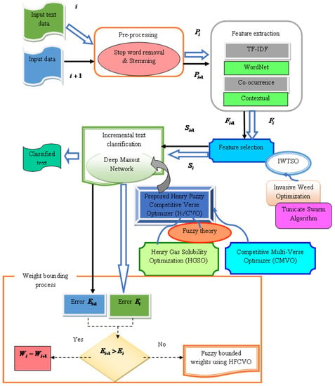
Figure 1.
Schematic view of proposed HFCVO-based DMN for incremental text classification.
3.1. Acquisition of Input Text Data
Let us consider the training dataset as with the number of training samples and it is expressed as,
where indicates the overall count of text documents and denotes the input data.
3.2. Pre-Processing Using Stop Word Removal and Stemming
The input text data is forwarded to the pre-processing phase, where redundant words are eliminated from the text data by employing two processes, namely, stop word removal and the stemming process. The occurrence of noises in the text data is due to unstructured data, and it is very necessary to eliminate the noises and redundant information from input data before performing the classification task. At this phase, data in the unstructured format are transformed into structured text representation for easy processing.
3.2.1. Stop Word Removal
Stop word is a division of the natural language processing system and stop words are words that contain articles, prepositions, or pronouns. Generally, words that do not contain any meaning are considered stop words. Stop word removal is the technique of eliminating unwanted or redundant words from a large database. It avoids the often occurring words that do not have any specific importance.
3.2.2. Stemming
By removing prefixes and suffixes, the stemming mechanism breaks down words into their stems at the root or base of the word. Stemming is an essential technique used to reduce words to their underlying words. For the purpose of distilling the words to their essence, many words are prepared. The pre-processed output of the input data is identified as , which is denoted as when it has undergone the feature extraction procedure. The pre-processing step is finished, and then the text in the text document is identified.
3.3. Feature Extraction
The pre-processed output is regarded as the starting point for the feature extraction procedure, which is how the important features are discovered. Wordnet-based features, co-occurrence-based features, TF–IDF-based features, and contextual-based features make up the features.
3.3.1. Wordnet-Based Features
Wordnet [] is the frequently employed lexical resource for NLP tasks, such as text categorization, information retrieval, and text summarization. It is the network of principles in the form of word nodes that is arranged using the semantic relations between the words depending upon their meaning. However, the semantic relationship is the relation between the principles such that each node consists of a group of words known as subsets that represent the real-world concept. In addition, it is the pointers among the subsets. It is basically utilized to determine the subsets from the pre-processed text data . The feature extracted from wordnet-based features is specified as .
3.3.2. Co-Occurrence-Based Features
The co-occurrence term is defined as the utilization of term sets or item sets. It is also described as the occurrence of term sets from the text repository, and this feature is utilized for the set of words. It is represented as,
where implies the co-occurrence frequency of words and ,and denotes the frequency of the word . Moreover, represents the feature obtained from co-occurrence features.
3.3.3. TF–IDF
TF–IDF consists of two parts, TF and IDF, in which TF finds the frequency of individual words, and IDF specifies the frequency of a word that is available in the text document. If a word, such as ‘are’, ‘is’, ‘am’, occurs in various texts, then the IDF value is low. In another case, if a word occurs in a small number of texts, then the IDF value is low. Meanwhile, IDF is highly utilized to determine the importance of words []. Let us assume that TF specifies the word frequency and it is represented as
where specifies the count of entries in each class and indicates the overall count of entries.
The IDF implies the inverse text frequency and it is computed below,
where implies the total count of texts available in the corpus and symbolizes the overall count of text that consists of word in the repository. Accordingly, TF–IDF is given by,
3.3.4. Contextual-Based Features
The context-based technique determines the correlated words by isolating it from the non-correlating text for achieving efficient categorization results. Finding the fundamental phrases that gain semantic meaning and the context terms that provide correlative context is necessary to complete this endeavor. The basic terms play the role of indicators of the correlated document, whereas the contexts [] play the role of validators. The purpose of validators is used to assess whether the determined basic terms are indicators or not. Hence, the technique chooses the correlated and non-correlated documents from the training dataset. Generally, the basic terms are identified utilizing a technique called language modeling employed from data retrieval.
Let us consider with as relevant documents and as non-correlative documents. Let us consider and as the context term and key term, respectively.
(i) Key term identification: The language model for this approach is specified as and it is determined as follows,
where and represent the language model for and , respectively.
(ii) Context term identification: After identifying the fundamental terms, the method starts to perform the context term detection for each key term individually.
The procedures followed by the mechanism of context term determination are defined as follows:
Step 1: Enumerate all basic term occurrences for both correlative and non-correlative documents and .
Step 2: Apply a sliding window of dimension ; the terms close to are refined as context terms. The window dimension is specified as the context length.
Step 3: The obtained correlative and non-relevant terms are denoted as and , respectively. The set of relevant documents and non-relevant documents is specified as and .
Step 4: The score is evaluated for the individual term and it is expressed as follows,
where denotes the language model for the relevant document set, whereas represents the language model for the non-relevant document.
The extracted feature from contextual-based features is and it is given by,
However, the feature extracted from the text data is indicated as in such a way that it includes , respectively.
3.4. Feature Selection
After refining the desired features, the refined feature is subjected to feature selection, where significant features are chosen utilizing the developed IWTSO algorithm. However, IWTSO is devised by integrating the features of IWO [,] with the TSA []. By merging these optimization algorithms, it helps to enhance the classification accuracy and also results in high-quality text data. The IWO algorithm is a metaheuristic population-based algorithm, which is designed to determine the best solution for a mathematical function through randomness and mimicking the compatibility of a weed colony. Weeds are plants that are resistant to any environmental changes and the exasperating growth of weeds influences crops. Additionally, this algorithm is inspired by the agriculture sector, expressed as colonies of invasive weeds. On the other hand, the TSA is an algorithm that was inspired by a novel and mimics the swarm behavior and jet propulsion of tunicates throughout the forage and navigation phase. Bright marine creatures called tunicates produce light that may be seen from a great distance. The weed features of IWO are combined with the swarm behavior and jet propulsion of the TSA to improve the rate of optimization convergence and produce the optimum solution to the optimization problem. However, the feature selected by the proposed developed method is denoted as . It is noteworthy to observe that the features chosen by processing the data with a Reuter dataset have a size of with a total count of 19,043 documents. However, the features selected with 20Newgroup dataset have the dimension of from a total count of 19,997 documents, whereas the features chosen with real-time data have the dimension of from a total number of 5000 documents.
Solution encoding: Solution encoding is the representation of the solution vector that evaluates the choice of best-fit features in such a way . The refined feature is subjected to feature selection, and the feature selected by the proposed developed method is denoted as . Figure 2 shows how the solution encoding is done.
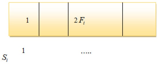
Figure 2.
Solution encoding.
Fitness function: The fitness parameter is exploited to identify the best feature among the set of features by considering the accuracy metric. The expression for accuracy is represented as,
where, specifies true positive, denotes true negative, indicates false positive, and implies false negative.
The algorithmic steps in IWTSO are explained below:
Step 1: Initialization
Let us initialize the population of weeds in the dimensional space as and the best position of the weed is denoted as .
Step 2: Compute the fitness function
The fitness parameter is utilized to determine the best solution by choosing the best features from a group of features.
Step 3: Update solution
The updated position of the weed in the improved IWO is expressed as follows,
The standard expression of the TSA is computed as,
Let us assume
As is the optimal search agent in the TSA, it can be replaced with the of the improved IWO.
where
where and imply the vector and gravity force, respectively. denotes the social force among the search agents, specifies the water flow advection, and indicates the random value that lies in the limit of . Moreover, the random number , , and lies within the limit of . Therefore, the value of and is set to 1 and 4, respectively.
Step 4: Determine the feasibility
The fitness function is determined for individual solutions and a solution with the optimal fitness measure is considered as the best solution.
Step 5: Termination
The aforementioned steps are continued until the best solution is achieved so far. Algorithm 1 elucidates the pseudocode of IWTSO.
| Algorithm 1. Pseudocode of proposed IWTSO. | |
| Sl. No | Pseudocode of IWTSO |
| 1 | Input:, |
| 2 | Output: |
| 3 | Initialize the weed population |
| 4 | Determine fitness function |
| 5 | Update the solution using Equation (14) |
| 6 | Determine the feasibility |
| 7 | Termination |
3.5. Arrival of New Data
When new data arrive, it is subjected to the pre-processing module, then the feature extraction module, followed by the feature selection module. These steps are explained in Section 3. The fuzzy-based incremental learning is performed by computing the error between the original data and the incremental or newly arrived data .
3.6. Incremental Text Classification Using HFCVO-Based DMN
The selected optimal feature is passed to the incremental text classification phase, where the process is done using the Deep Maxout Network. However, the network is trained by exploiting the developed HFCVO algorithm, such that the optimal weight of the classifier is increased. By doing so, the performance of text classification is accurate.
3.6.1. Architecture of Deep Maxout Network
The DMN [] is a type of trainable activation parameter with a multi-layer structure. Let us consider an input , which is a raw input vector of a hidden layer. Here, the DMN consists of layers, such as input, convolutional, dropout, max pooling layer, dense, maxout layer, and output layer. When an input with the dimension of is fed into the input neurons of the input layer, it produces an output of . The process is continued by the dropout layer and the convolutional layer, alternatively. The final dropout layer generates an output with a dimension of , which is considered an input to the dense layer. Subsequently, the final output of the DMN is denoted as with a dimension of .
The activation function of a hidden unit is mathematically computed as,
where denotes the total count of units present in the layer and implies the overall count of layers in the DMN. An arbitrary continuous activation parameter can be roughly approximated by the DMN activation function. To mimic the DMN structure, the traditional activation parameters’ ReLU and an absolute value rectifier are utilized. The ReLu is initially considered in RBM and it is expressed as,
where implies the input, whereas is the output.
The maxout is an extended ReLU, which performs the maximum function of the trainable linear function. The output achieved by a maxout unit is formulated below,
In a CNN, activation of a maxout unit is equivalent to feature maps. Although the maxout unit is equivalent to generally employed spatial max-pooling in CNNs, it consumes a large amount of time over trainable functions. Figure 3 portrays the architecture of the DMN.
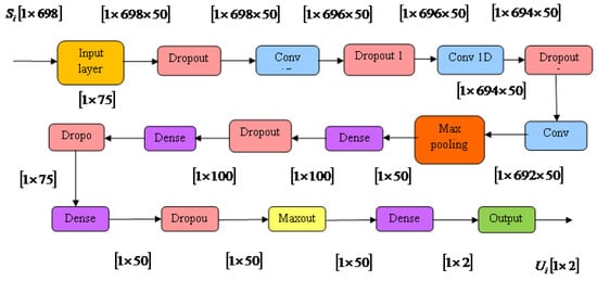
Figure 3.
Structure of the DMN.
3.6.2. Error Estimation
Error estimation of the original data utilized for text classification is determined using the following equation,
where denotes the total count of samples, and and indicate the targeted output and the result gained from the network classifier DMN.
3.6.3. Fuzzy Bound-Based Incremental Learning
When newly arrived data is included in the network, error is computed, and the weights are to be upgraded without learning the earlier occurrence. Then, compare the incremental data error with the original data error . If the error value of the incremental data is less than that of the original data, then immediately the weights are bounded based on the fuzzy bound approach, and the optimal weights are updated using the proposed HFCVO.
Based on the measurements given to the factors, can be achieved and the fuzzy bound is computed.
3.6.4. Weight Update Using Proposed HFCVO
In order to bound the weights, the optimal weights are updated using a newly proposed algorithm named HFCVO. This hybrid optimization algorithm is achieved by integrating the features of HGSO [] and CMVO [] with a fuzzy concept []. The revolutionary population-based metaheuristic algorithm known as HGSO is entirely based on physics principles. Additionally, this optimization is based on Henry’s law, which states that at a constant temperature, the capacity of a liquid and the amount of a particular gas that dissolves are proportional to half pressure. Due to this characteristic, HGSO is highly sought-after for addressing complex optimization problems with a variety of local best solutions. On the other hand, CMVO is an effective population-based optimization strategy that integrates the MVO with the idea of a pair-wise competition mechanism between universes. This algorithm increases the search capability and enhances the exploration and exploitation phases. By integrating this immense optimization algorithm, it generates promising results in updating the optimal weights.
Solution encoding: Solution encoding is used to represent the solution of a vector and here the optimal weights are determined using the solution vector. Here, is the solution vector in which represents the learning parameter.
The algorithmic procedure involved in this process is deliberated in the below steps:
Step 1: Initialization
Let us initialize the population of gases in the dimensional search space and the location of gases is initialized depending upon the below expression,
where denotes the solution in the search space, is a random measure that lies in the limit of , and and are the maximum and minimum bounds, respectively. Moreover, represents the iteration period. The Henry’s constant and partial pressure of gas in the cluster is represented as follows,
where and are constant values. and are the partial pressure of gas and the constant value of type .
Step 2: Fitness function
The fitness function is used to determine the optimal solution using Equation (26).
Step 3: Clustering
The search agents are equally partitioned into a number of gas categories. Every cluster possesses equivalent gases and, hence, it has an equivalent Henry’s constant measure.
Step 4: Evaluation
Every cluster is estimated to determine the best solution of gas that attains the maximum equilibrium state. After that, the gases are ordered in a hierarchical ranking to achieve the optimal gas.
Step 5: Update Henry’s coefficient
Henry’s coefficient is upgraded based on the below expression,
where implies that Henry’s coefficient for cluster , is the temperature, and specifies the iteration number.
Step 6: Update the solubility of gas
The solubility of gas is upgraded depending on computing the below equation,
where SOp,q is the gas solubility of p in cluster q, is the partial pressure on gas in cluster , and is a constant.
Step 7: Update the position
The location of Henry gas solubility is updated as follows:
From CMVO, the best universe through wormhole tunnels is given by,
Multiplying and inside the parentheses,
Substituting Equation (43) in Equation (38), the equation is given as,
Hence, the update solution becomes,
where represents the position of gas in cluster , and and imply the best gas in cluster and the best gas in the swarm, respectively. denotes the winner universe in the iteration, and the mean position value of the corresponding universe is expressed as . Moreover, implies the traveling distance rate.
Step 8: Escape from the local optimum
To leave the local location, one uses this local optimum. It can be described by the following equation:
where is the total count of search agents.
Step 9: Update the location of the worst agents
The location of the worst agents is updated as follows,
where denotes the location of gas in cluster , and and are the bounds of the problem.
Step 10: Termination
The algorithmic steps are continued until it achieves a suitable solution. Algorithm 2 elucidates the pseudocode of the developed HFCVO algorithm.
| Algorithm 2. Pseudocode of proposed HFCVO. | |
| SL. No. | Pseudocode of HFCVO |
| 1 | Input:, , , , and Output: |
| 2 | Begin |
| 3 | The population agents are divided into various gas kinds using Henry’s constant value |
| 4 | Determine each cluster |
| 5 | Obtain the best gas in each cluster and optimal search agent |
| 6 | for search agent do |
| 7 | Update all search agents’ positions using equation (50) |
| 8 | end for |
| 9 | Update each gas type’s Henry’s coefficient using Equation (34) |
| 10 | Utilizing Equation (35), update the solubility of gas |
| 11 | Utilizing Equation (51), arrange and select the number of worst agents |
| 12 | Using Equation (52), update the location of the worst agents |
| 13 | Update the best gas and best search agent |
| 14 | end while |
| 15 | |
| 16 | Return |
| 17 | Terminate |
4. Results and Discussion
This section explains how the created HFCVO-based DMN was evaluated in compliance with evaluation measures.
4.1. Experimental Setup
The implementation of the HFCVO-based DBN is done in the PYTHON tool. Table 1 shows the PYTHON libraries.

Table 1.
PYTHON Libraries.
4.2. Dataset Description
The datasets utilized for the implementation purpose are the Reuter dataset [], 20-Newsgroup dataset [], and the real-time dataset.
Reuter dataset: There are 21,578 cases in this dataset, and 19,043 documents were picked for the classification job. Depending on the categories of documents, groups and indexes are created here. It has five attributes, 206,136 web hits, and no missing values.
20-Newsgroup dataset: It is well recognized for its demonstrations of text appliances for machine learning techniques, including text clustering and text categorization, in a collection of newsgroup documents. In this case, duplicate messages are eliminated to reveal the headers “from” and “subject” on the original messages.
Real-time data: For each of the 20 topics chosen, 250 publications are gathered from the Springer and Science Directwebsites. Only a few of the topics include developments in data analysis, artificial intelligence, big data, bioinformatics, biometrics, cloud computing, and other concepts. 5000 documents are therefore included in the text categorization process.
4.3. Performance Analysis
This section describes the performance assessment of the developed HFCVO-based DMN with respect to evaluation metrics using three datasets.
4.3.1. Analysis Using Reuter Dataset
Table 2 illustrates the performance assessment of the HFCVO-based DBN utilizing the Reuter dataset. If the training percentage is 90%, the TPR obtained by the proposed HFCVO-based DBN with a feature size of 100 is 0.873, a feature size of 200 is 0.897, a feature size of 300 is 0.901, a feature size of 400 is 0.928, and afeature size of 500 is 0.935. By taking the training percentage as 90%, the proposed HFCVO-based DBN achieved aTNR of 0.858 for a feature size of 100, 0.874 for a feature size of 200, 0.896 for a feature size of 300, 0.902 for a feature size of 400, and 0.925 for a feature size of 500. By considering the training percentage as 90%, the FNR obtained by the proposed HFCVO-based DBN with a feature size of 100, 200, 300, 400, and 500 is 0.127, 0.103, 0.099, 0.072, and 0.065, respectively. If the training percentage is 90%, the precision attained by the developed HFCVO-based DBN with a feature size of 100 is 0.883, 200 is 0.909, 300 is 0.923, 400 is 0.947, and 500 is 0.970. If the training data is 90%, the testing accuracy achieved by the developed HFCVO-based DBN with a feature size 100 is 0.857, with a feature size of 200 is 0.878, with a feature size of 300 is 0.898, with a feature size of 400 is 0.905, and with a feature size of 500 is 0.924.
Table 2.
Performance analysis using Reuter dataset for TPR, TNR, FNR, precision, and testing accuracy.
4.3.2. Analysis Using 20Newsgroup Dataset
Table 3 depicts the assessment of the HFCVO-based DBN utilizing the 20 Newsgroup dataset. For a training percentage of 90%, the TPR yielded by the HFCVO-based DBN with a feature size of 100 is 0.894, with a feature size of 200 is 0.913, with a feature size of 300 is 0.935, with a feature size of 400 is 0.947, and with a feature size of 500 is 0.963. If the training percentage is maximized to 90%, the developed HFCVO-based DBN attained aTNR of 0.878 for a feature size of 100, 0.888 for a feature size of 200, 0.909 for a feature size of 300, 0.919 for a feature size of 400, and 0.939 for a feature size of 500. By assuming the training data as 90%, the FNR achieved by the proposed HFCVO-based DBN with a feature size of 100 is 0.106, 200 is 0.087, 300 is 0.065, 400 is 0.053, and 500 is 0.037, respectively. If the training data is 90%, the precision attained by the proposed HFCVO-based DBN with a feature size of 100 is 0.891, 200 is 0.918, 300 is 0.938, 400 is 0.955, and 500 is 0.974. By considering the training data as 90%, the testing accuracy yielded by the proposed HFCVO-based DBN with a feature size of 100, with a feature size of 200, with a feature size of 300, with a feature size of 400, and with a feature size of 500 is 0.871, 0.899, 0.918, 0.938, and 0.956, respectively.
Table 3.
Performance analysis using 20Newsgroup Dataset for TPR, TNR, FNR, precision, and testing accuracy.
4.3.3. Analysis Using Real-Time Dataset
Table 4 depicts the performance assessment of the developed HFCVO-based DBN utilizing the Real-time dataset. If the training percentage is 90%, the TPR obtained by the proposed HFCVO-based DBN with a feature of size = 100 is 0.869, with a feature size of 200 is 0.897, with a feature size of 300 is 0.929, with a feature size of 400 is 0.949, and with a feature size of 500 is 0.968. If the training percentage is increased to 90%, the proposed HFCVO-based DBN achieved a TNR of 0.865 for a feature size of 100, 0.886 for a feature size of 200, 0.908 for a feature size of 300, 0.926 for a feature size of 400, and 0.941 for a feature size of 500. By considering the training data as 90%, the FNR obtained by the proposed HFCVO-based DBN with a feature size of 100, 200, 300, 400, and 500 is 0.131, 0.103, 0.071, 0.051, and 0.032, respectively. If the training data is 90%, the precision attained by the proposed HFCVO-based DBN with a feature size of 100 is 0.878, 200 is 0.892, 300 is 0.919, 400 is 0.939, and 500 is 0.954. By considering the training percentage as 90%, the testing accuracy obtained by the proposed HFCVO-based DBN with a feature size of 100 is 0.884, with a feature size of 200 is 0.901, a feature size of 300 is 0.928, a feature size of 400 is 0.944, and a feature size of 500 is 0.955.
Table 4.
Performance analysis using Real-time dataset for TPR, TNR, FNR, precision, and testing accuracy.
4.4. Comparative Methods
The performance enhancement of the HFCVO-based DBN is compared with existing approaches, such as the SGrC-based DBN [], MB–FF-based NN [], LFNN [], and SVNN [].
4.5. Comparative Analysis
This section deliberates the comparative assessment of the developed HFCVO-based DBN in terms of the evaluation metrics using three datasets.
4.5.1. Analysis Using Reuter Dataset
Table 5 represents the assessment of the developed method by employing the Reuter dataset. When the training percentage is 90%, the TPR obtained by the proposed HFCVO-based DBN is 0.935, which results in a performance increment of the developed method compared with that of traditional approaches; for example, that compared with the SGrC-based DBN is 14.035%, the MB–FF-based NN is 9.652%, the LFNN is 6.510%, and the SVNN is 4.276%. If the training percentage is 90%, the TNR obtained by conventional methods, such as the SGrC-based DBN, MB–FF-based NN, LFNN, and SVNN, is 0.798, 0.814, 0.837, and 0.854, respectively. By considering the training percentage as 90%, the FNR attained by the developed method is 0.065, whereas the traditional methods attained an FNR of 0.196 for the SGrC-based DBN, 0.155 for the MB–FF-based NN, 0.125 for the LFNN, and 0.105 for the SVNN. If the training percentage is 90%, the precision achieved by the proposed method is 0.970, which reveals a performance development of the developed method compared with that of existing methods; for example, that compared with the SGrC-based DBN is 20.218%, the MB–FF-based NN is 19.164%, the LFNN is 13.915%, and the SVNN is 6.397%. The testing accuracy achieved by the proposed HFCVO-based DBN is 0.924 when the training data = 90%.
Table 5.
Comparative analysis using Reuter dataset for TPR, TNR, FNR, precision, and testing accuracy.
4.5.2. Analysis Using 20Newsgroup Dataset
Table 6 represents an assessment of the proposed method utilizing the 20 Newsgroup dataset. When the training percentage is 90%, the TPR obtained by the proposed HFCVO-based DBN is 0.963,which indicates the development of the proposed method compared with the classical schemes; for example, that compared with the SGrC-based DBN is 14.052%, the MB–FF-based NN is 11.038%, the LFNN is 7.692%, and the SVNN is 5.617%. If the training data is 90%, the TNR obtained by conventional methods, such as the SGrC-based DBN, MB–FF-based NN, LFNN, and SVNN, is 0.836, 0.860, 0.889, and 0.909. By assuming the training percentage as 90%, the FNR achieved by the developed technique is 0.037, while the traditional schemes attained an FNR of 0.173 for the SGrC-based DBN, 0.144 for the MB–FF-based NN, 0.111 for the LFNN, and 0.091 for the SVNN. If the training data is 90%, the precision yielded by the developed strategy is 0.974, which reveals a performance enhancement of the developed method compared with that of conventional methods; for example, that compared with the SGrC-based DBN is 19.377%, the MB–FF-based NN is 18.126%, the LFNN is 12.203%, and the SVNN is 5.923%. The testing accuracy attained by the proposed HFCVO-based DBN is 0.956 when the training data = 90%.
Table 6.
Comparative analysis using 20-Newsgroup Dataset for TPR, TNR, FNR, Precision, and testing accuracy.
4.5.3. Analysis Using Real-Time Dataset
Table 7 represents the assessment of the developed method using the Real-time dataset. When the training percentage is 90%, the TPR obtained by the proposed HFCVO-based DBN is 0.968,which indicates a performance enhancement of proposed method compared with that of conventional approaches; for example, that compared with the SGrC-based DBN is 13.425%, the MB–FF-based NN is 10.761%, the LFNN is 7.116%, and the SVNN is 5.709%. If the training percentage is 90%, the TNR obtained by conventional methods, such as the SGrC-based DBN, the MB–FF-based NN, the LFNN, and the SVNN is 0.802, 0.824, 0.855, and 0.897. By considering the training percentage as 90%, the FNR achieved by the developed model is 0.032, while the traditional techniques attained an FNR of 0.162 for the SGrC-based DBN, 0.137 for the MB–FF-based NN, 0.101 for the LFNN, and 0.088 for the SVNN. If the training percentage is 90%, the precision obtained by the proposed method is 0.954, which reveals the performance increment of the developed method compared with that of conventional techniques; for example, that compared with the SGrC-based DBN is 17.608%, the MB–FF-based NN is 15.868%, the LFNN is 11.299%, and the SVNN is 1.846%. The testing accuracy achieved by the proposed HFCVO-based DBN is 0.955 when the training data = 90%.
Table 7.
Comparative analysis using Real-time dataset for TPR, TNR, FNR, precision, and testing accuracy.
4.6. Analysis Based on Optimization Techniques
This section deliberates the assessment of the developed HFCVO-based DBM based on optimization techniques using three datasets. The algorithms utilized in this analysis are TSO + DMN [], IIWO + DMN [], IWTSO + DMN, HGSO + DMN [], and CMVO + DMN [].
4.6.1. Analysis Using Reuter Dataset
Table 8 shows the assessment of the optimization methodologies in terms of performance metrics. If the training data is 90%, the TPR obtained by the developed HFCVO + DMN is 0.935, whereas the TPR attained by TSO + DMN is 0.865, IIWO + DMN is 0.875, IWTSO + DMN is 0.887, HGSO + DMN is 0.899, and CMVO + DMN is 0.914. If the training data is 90%, the TNR obtained by the optimization algorithms, such as TSO + DMN, IIWO + DMN, IWTSO + DMN, HGSO + DMN, and CMVO + DMN, is 0.835, 0.854, 0.865, 0.887, and 0.905, respectively. By assuming the training percentage as 90%, the FNR yielded by the proposed HFCVO + DMN is 0.065, whereas the other optimization algorithms obtained an FNR of 0.135 for TSO + DMN, 0.125 for IIWO + DMN, 0.113 for IWTSO + DMN, 0.101 for HGSO + DMN, and 0.086 for CMVO + DMN. When the training percentage is maximized to 90%, the precision obtained by the developed HFCVO + DMN is 0.970. If the training percentage is elevated to 90%, the proposed HFCVO + DMN attained a testing accuracy of 0.924, whereas the conventional methodologies obtained a testing accuracy of 0.854 for TSO + DMN, 0.865 for IIWO + DMN, 0.875 for IWTSO + DMN, 0.898 for HGSO + DMN, and 0.905 for HFCVO + DMN.
Table 8.
Analysis based on optimization using Reuter dataset for TPR, TNR, FNR, precision, and testing accuracy.
4.6.2. Analysis Using 20Newsgroup Dataset
Table 9 specifies the assessment of the optimization methodologies in accordance with the performance measures. When the training data = 90%, the TPR yielded by the developed HFCVO + DMN is 0.963, while the TPR obtained by TSO + DMN is 0.887, IIWO + DMN is 0.904, IWTSO + DMN is 0.914, HGSO + DMN is 0.933, and CMVO + DMN is 0.954. By considering the training percentage as 90%, the TNR achieved by the optimization methodologies such as TSO + DMN is 0.841, IIWO + DMN is 0.865, IWTSO + DMN is 0.885, HGSO + DMN is 0.895, and CMVO + DMN is 0.925. By assuming the training percentage as 90%, the FNR attained by the developed HFCVO + DMN is 0.037, whereas the other optimization techniques achieved an FNR of 0.113 for TSO + DMN, 0.096 for IIWO + DMN, 0.086 for IWTSO + DMN, 0.067 for HGSO + DMN, and 0.046 for CMVO + DMN. When the training percentage = 90%, the proposed HFCVO + DMN obtained a precision of 0.974. When the training percentage is increased to 90%, the proposed HFCVO + DMN attained a testing accuracy of 0.956, whereas the conventional methodologies obtained a testing accuracy of 0.857 for TSO + DMN, 0.875 for IIWO + DMN, 0.885 for IWTSO + DMN, 0.937 for HGSO + DMN, and 0.941 for HFCVO + DMN.
Table 9.
Analysis based on optimization using 20Newsgroup dataset for TPR, TNR, FNR, precision, and testing accuracy.
4.6.3. Analysis Using Real-Time Dataset
Table 10 represents the assessment of the optimization methodologies in terms of the performance metrics. By considering the training percentage is 90%, the TPR obtained by HFCVO + DMN is 0.968, whereas the TPR attained by TSO + DMN is 0.875, IIWO + DMN is 0.885, IWTSO + DMN is 0.904, HGSO + DMN is 0.925, and CMVO + DMN is 0.941. If the training data is 90%, the TNR obtained by the optimization algorithms, such as TSO + DMN, IIWO + DMN, IWTSO + DMN, HGSO + DMN, and CMVO + DMN, is 0.865, 0.875, 0.895, 0.921, and 0.933, respectively. By considering the training percentage as 90%, the FNR yielded by the proposed HFCVO + DMN is 0.032, whereas the other optimization algorithms obtained an FNR of 0.125 for TSO + DMN, 0.115 for IIWO + DMN, 0.075 for IWTSO + DMN, 0.059 for HGSO + DMN, and0.032 for CMVO + DMN. When the training percentage is maximized to 90%, the precision obtained by the developed HFCVO + DMN is 0.954. If the training percentage is elevated to 90%, the proposed HFCVO + DMN attained a testing accuracy of 0.955, whereas the conventional methodologies obtained a testing accuracy of 0.865 for TSO + DMN, 0.885 for IIWO + DMN, 0.895 for IWTSO + DMN, 0.926 for HGSO + DMN, and 0.935 for HFCVO + DMN.
Table 10.
Analysis based on optimization using Real-time dataset for TPR, TNR, FNR, precision, and testing accuracy.
5. Conclusions
Text mining has been considered a significant tool for diverse knowledge discovery-based applications, such as document arrangement, fake email filtering, and news groupings. Nowadays, text mining employs incremental learning data, as they are economically cost-effective when handling massive data. However, the major crisis that occurs in incremental learning is low accuracy because of the existence of countless terms in the text document. Deep learning is an effectual technique for refining underlying data in the text but it provides superior results on closed datasets than real-world data. Hence, approaches to deal with imbalanced datasets are very significant for addressing such problems. Hence, this research proposes an effective incremental text classification strategy using the proposed HFCVO-based DMN. The proposed approach consists of four phases, namely, pre-processing, feature extraction, feature selection, and incremental text categorization. Here, the optimal features are extracted using the developed IWTSO algorithm. Moreover, the incremental text classification is done by exploiting the DBN, where the network is trained using HFCVO. When incremental data arrive, the error is computed for both the original data and incremental data. If the error of the incremental data is less than the error of the original data, then the weights are bounded based on a fuzzy theory using the same proposed HFCVO. The proposed algorithm is devised by merging the features of HGSO and CMVO with the fuzzy concept. Meanwhile, the proposed HFCVO-based DNM achieved a maximum TPR of 0.968, a maximum TNR of 0.941, a low FNR of 0.032, a high precision of 0.954, and a high accuracy of 0.955.
Author Contributions
Conceptualization, G.S. and A.N.; methodology, G.S.; software, G.S.; validation, G.S. and A.N.; formal analysis, G.S.; investigation, G.S.; resources, G.S.; data curation, G.S.; writing—original draft preparation, G.S.; writing—review and editing, G.S..; visualization, G.S.; supervision, G.S.; project administration, G.S.; funding acquisition, A.N. All authors have read and agreed to the published version of the manuscript.
Funding
This research received no external funding.
Institutional Review Board Statement
Not applicable.
Informed Consent Statement
Not applicable.
Data Availability Statement
The data presented in this study are openly available in “https://archive.ics.uci.edu/ml/datasets/reuters-21578+text+categorization+collection” (accessed on 23 January 2022), reference number [] and “https://www.kaggle.com/crawford/20-newsgroups” (accessed on 23 January 2022), reference number [].
Conflicts of Interest
The authors declare no conflict of interest.
Nomenclature
| Abbreviations | Descriptions |
| HFCVO | Henry Fuzzy Competitive Multi-verse Optimizer |
| DMN | Deep Maxout Network |
| IWTSO | Invasive Weed Tunicate Swarm Optimization |
| DMN | Deep Maxout Network |
| IWO | Invasive Weed Optimization |
| NB | Naïve Bayes |
| TSA | Tunicate Swarm Algorithm |
| DMN | Deep Maxout Network |
| HGSO | Henry Gas Solubility Optimization |
| CMVO | Competitive Multi-Verse Optimizer |
| WWW | World Wide Web |
| ML | Machine Learning |
| TNR | True Negative Rate |
| SVM | Support Vector Machine |
| FNR | False Negative Rate |
| KNN | K-Nearest Neighbor |
| AC | Associative Classification |
| SGrC-based DBN | Spider Grasshopper Crow Optimization Algorithm-based Deep Belief Neural network |
| SMO | Spider Monkey Optimization |
| GCOA | Grasshopper Crow Optimization Algorithm |
| RL | Reinforcement Learning |
| SVNN | Support Vector Neural Network |
| LSTM | Long Short-Term Memory |
| MB–FF-based NN | Monarch Butterfly optimization–FireFly optimization-based Neural Network |
| TF–IDF | Term Frequency–Inverse Document Frequency |
| ST | Sequential Targeting |
| COA | Cuckoo Optimization Algorithm |
| Gibbs MedLDA | Interactive visual assessment model depending on a semi-supervised topic modeling technique called allocation. |
| SG–CAV-based DBN | Stochastic Gradient–CAViaR-based Deep Belief Network |
| ReLU | Rectified Linear Unit |
| RBM | Restricted Boltzmann Machines |
| MVO | Multi-Verse Optimizer algorithm |
| NN | Neural Network |
| TPR | True Positive Rate |
| RF | Random Forest |
| NLP | Natural Language Processing |
References
- Yan, Y.; Tao, Y.; Jin, S.; Xu, J.; Lin, H. An Interactive Visual Analytics System for Incremental Classification Based on Semi-supervised Topic Modeling. In Proceedings of the IEEE Pacific Visualization Symposium (PacificVis), Bangkok, Thailand, 23–26 April 2019; pp. 148–157. [Google Scholar]
- Chander, S.; Vijaya, P.; Dhyani, P. Multi kernel and dynamic fractional lion optimization algorithm for data clustering. Alex. Eng. J. 2018, 57, 267–276. [Google Scholar] [CrossRef]
- Jadhav, A.N.; Gomathi, N. DIGWO: Hybridization of Dragonfly Algorithm with Improved Grey Wolf Optimization Algorithm for Data Clustering. Multimed. Res. 2019, 2, 1–11. [Google Scholar]
- Tan, A.H. Text mining: The state of the art and the challenges. In Proceedings of the Pakdd 1999 Workshop on Knowledge Discovery from Advanced Databases, Beijing, China, 26–28 April 1999; Volume 8, pp. 65–70. [Google Scholar]
- Yadav, P. SR-K-Means clustering algorithm for semantic information retrieval. Int. J. Invent. Comput. Sci. Eng. 2014, 1, 17–24. [Google Scholar]
- Sailaja, N.V.; Padmasree, L.; Mangathayaru, N. Incremental learning for text categorization using rough set boundary based optimized Support Vector Neural Network. In Data Technologies and Applications; Emerald Publishing Limited: Bingley, UK, 2020. [Google Scholar]
- Kaviyaraj, R.; Uma, M. Augmented Reality Application in Classroom: An Immersive Taxonomy. In Proceedings of the 2022 4th International Conference on Smart Systems and Inventive Technology (ICSSIT), Tirunelveli, India, 20 January 2022; pp. 1221–1226. [Google Scholar]
- Vidyadhari, C.; Sandhya, N.; Premchand, P. A Semantic Word Processing Using Enhanced Cat Swarm Optimization Algorithm for Automatic Text Clustering. Multimed. Res. 2019, 2, 23–32. [Google Scholar]
- Sebastiani, F. Machine learning in automated text categorization. ACM Comput. Surv. 2022, 34, 1–47. [Google Scholar] [CrossRef]
- Srilakshmi, V.; Anuradha, K.; Bindu, C.S. Incremental text categorization based on hybrid optimization-based deep belief neural network. J. High Speed Netw. 2021, 27, 1–20. [Google Scholar] [CrossRef]
- Jo, T. K nearest neighbor for text categorization using feature similarity. Adv. Eng. ICT Converg. 2019, 2, 99. [Google Scholar]
- Sheu, J.J.; Chu, K.T. An efficient spam filtering method by analyzing e-mail’s header session only. Int. J. Innov. Comput. Inf. Control. 2009, 5, 3717–3731. [Google Scholar]
- Ghiassi, M.; Olschimke, M.; Moon, B.; Arnaudo, P. Automated text classification using a dynamic artificial neural network model. Expert Syst. Appl. 2012, 39, 10967–10976. [Google Scholar] [CrossRef]
- Wang, Q.; Fang, Y.; Ravula, A.; Feng, F.; Quan, X.; Liu, D. WebFormer: The Web-page Transformer for Structure Information Extraction. In Proceedings of the ACM Web Conference (WWW ’22), Lyon, France, 25–29 April 2022; pp. 3124–3133. [Google Scholar]
- Yan, L.; Ma, S.; Wang, Q.; Chen, Y.; Zhang, X.; Savakis, A.; Liu, D. Video Captioning Using Global-Local Representation. IEEE Trans. Circuits Syst. Video Technol. 2022, 32, 6642–6656. [Google Scholar] [CrossRef]
- Liu, D.; Cui, Y.; Tan, W.; Chen, Y. SG-Net: Spatial Granularity Network for One-Stage Video Instance Segmentation. In Proceedings of the IEEE/CVF Conference on Computer Vision and Pattern Recognition, Nashville, TN, USA, 21 June 2021. [Google Scholar]
- Al-diabat, M. Arabic text categorization using classification rule mining. Appl. Math. Sci. 2012, 6, 4033–4046. [Google Scholar]
- Srinivas, K. Prediction of e-learning efficiency by deep learning in E-khool online portal networks. Multimed. Res. 2020, 3, 12–23. [Google Scholar] [CrossRef]
- Alzubi, A.; Eladli, A. Mobile Payment Adoption-A Systematic Review. J. Posit. Psychol. Wellbeing 2021, 5, 565–577. [Google Scholar]
- Rupapara, V.; Narra, M.; Gunda, N.K.; Gandhi, S.; Thipparthy, K.R. Maintaining Social Distancing in Pandemic Using Smartphones With Acoustic Waves. IEEE Trans. Comput. Soc. Syst. 2022, 9, 605–611. [Google Scholar] [CrossRef]
- Rahul, V.S.; Kosuru; Venkitaraman, A.K. Integrated framework to identify fault in human-machine interaction systems. Int. Res. J. Mod. Eng. Technol. Sci. 2022, 4, 1685–1692. [Google Scholar]
- Gali, V. Tamil Character Recognition Using K-Nearest-Neighbouring Classifier based on Grey Wolf Optimization Algorithm. Multimed. Res. 2021, 4, 1–24. [Google Scholar] [CrossRef]
- Shirsat, P. Developing Deep Neural Network for Learner Performance Prediction in EKhool Online Learning Platform. Multimed. Res. 2020, 3, 24–31. [Google Scholar] [CrossRef]
- Shan, G.; Xu, S.; Yang, L.; Jia, S.; Xiang, Y. Learn#: A novel incremental learning method for text classification. Expert Syst. Appl. 2020, 147, 113198. [Google Scholar]
- Kayest, M.; Jain, S.K. An Incremental Learning Approach for the Text Categorization Using Hybrid Optimization; Emerald Publishing Limited: Bingley, UK, 2019. [Google Scholar]
- Jang, J.; Kim, Y.; Choi, K.; Suh, S. Sequential Targeting: An incremental learning approach for data imbalance in text classification. arXiv 2020, arXiv:2011.10216. [Google Scholar]
- Nihar, M.R.; Midhunchakkaravarthy, J. Evolutionary and Incremental Text Document Classifier using Deep Learning. Int. J. Grid Distrib. Comput. 2021, 14, 587–595. [Google Scholar]
- Srilakshmi, V.; Anuradha, K.; Bindu, C.S. Stochastic gradient-CAViaR-based deep belief network for text categorization. Evol. Intell. 2020, 14, 1727–1741. [Google Scholar] [CrossRef]
- Nihar, M.R.; Rajesh, S.P. LFNN: Lion fuzzy neural network-based evolutionary model for text classification using context and sense based features. Appl. Soft Comput. 2018, 71, 994–1008. [Google Scholar]
- Liu, Y.; Sun, C.J.; Lin, L.; Wang, X.; Zhao, Y. Computing semantic text similarity using rich features. In Proceedings of the 29th Pacific Asia Conference on Language, Information and Computation, Shanghai, China, 30 October–1 November 2015; pp. 44–52. [Google Scholar]
- Wu, D.; Yang, R.; Shen, C. Sentiment word co-occurrence and knowledge pair feature extraction based LDA short text clustering algorithm. J. Intell. Inf. Syst. 2020, 56, 1–23. [Google Scholar] [CrossRef]
- Zhou, Y.; Luo, Q.; Chen, H.; He, A.; Wu, J. A discrete invasive weed optimization algorithm for solving traveling salesman problem. Neurocomputing 2015, 151, 1227–1236. [Google Scholar] [CrossRef]
- Sang, H.Y.; Duan, P.Y.; Li, J.Q. An effective invasive weed optimization algorithm for scheduling semiconductor final testing problem. Swarm Evol. Comput. 2018, 38, 42–53. [Google Scholar] [CrossRef]
- Kaur, S.; Awasthi, L.K.; Sangal, A.L.; Dhiman, G. Tunicate Swarm Algorithm: A new bio-inspired based metaheuristic paradigm for global optimization. Eng. Appl. Artif. Intell. 2020, 90, 103541. [Google Scholar] [CrossRef]
- Sun, W.; Su, F.; Wang, L. Improving deep neural networks with multi-layer maxout networks and a novel initialization method. Neurocomputing 2018, 278, 34–40. [Google Scholar] [CrossRef]
- Hashim, F.A.; Houssein, E.H.; Mabrouk, M.S.; Al-Atabany, W.; Mirjalili, S. Henry gas solubility optimization: A novel physics-based algorithm. Future Gener. Comput. Syst. 2019, 101, 646–667. [Google Scholar] [CrossRef]
- Benmessahel, I.; Xie, K.; Chellal, M. A new competitive multiverse optimization technique for solving single-objective and multi-objective problems. Eng. Rep. 2020, 2, e12124. [Google Scholar]
- Reuters-21578 Text Categorization Collection Data Set. Available online: https://archive.ics.uci.edu/ml/datasets/reuters-21578+text+categorization+collection (accessed on 23 January 2022).
- 20 Newsgroup Dataset. Available online: https://www.kaggle.com/crawford/20-newsgroups (accessed on 23 January 2022).
Disclaimer/Publisher’s Note: The statements, opinions and data contained in all publications are solely those of the individual author(s) and contributor(s) and not of MDPI and/or the editor(s). MDPI and/or the editor(s) disclaim responsibility for any injury to people or property resulting from any ideas, methods, instructions or products referred to in the content. |
© 2023 by the authors. Licensee MDPI, Basel, Switzerland. This article is an open access article distributed under the terms and conditions of the Creative Commons Attribution (CC BY) license (https://creativecommons.org/licenses/by/4.0/).