Article

An Efficient Path Planning Algorithm Using a Potential Field for Ground Forces

Department of Operations Research, Korea National Defence University (KNDU), Nonsan 33021, Republic of Korea
*
Author to whom correspondence should be addressed.
Computation 2023, 11(1), 12; https://doi.org/10.3390/computation11010012
Submission received: 22 December 2022 / Revised: 6 January 2023 / Accepted: 9 January 2023 / Published: 11 January 2023

Abstract

:
With the development and proliferation of unmanned weapons systems, path planning is becoming increasingly important. Existing path-planning algorithms mainly assume a well-known environment, and thus pre-planning is desirable, but the actual ground battlefield is uncertain, and numerous contingencies occur. In this study, we present a novel, efficient path-planning algorithm based on a potential field that quickly changes the path in a constantly changing environment. The potential field is composed of a set of functions representing enemy threats and a penalty term representing distance to the target area. We also introduce a new threat function using a multivariate skew-normal distribution that accurately expresses the enemy threat in ground combat.

1. Introduction

Unmanned systems such as robotics, autonomous vehicles, and UGVs (unmanned ground vehicles) have been widely used in commercial and industrial applications. Among the various technologies applied to unmanned systems, one of the most important is path planning, a method for planning paths to move an object from a start point to an end point while avoiding obstacles. Path planning can be applied to various environments with diverse obstacles. Kumar et al. [1] applied path planning to shelves as obstacles in a warehouse, and Hu et al. [2] considered cars as obstacles on a road. In such environments, the general path-planning procedure starts with analyzing prior information about the given environment, defining the space (whether discrete or continuous), and implementing obstacles depending on the defined space. Then, algorithms are applied to plan the path. Based on this general path planning concept, existing studies suggest various methods depending on the environment where their experiments are placed. For example, ŠIŠLÁK et al. [3] planned a path on a 2-dimensional discrete space targeting a robotics using A* algorithm. Iswanto et al. [4] targeted a quadrotor model to plan a path on a 3-dimensional continuous space.
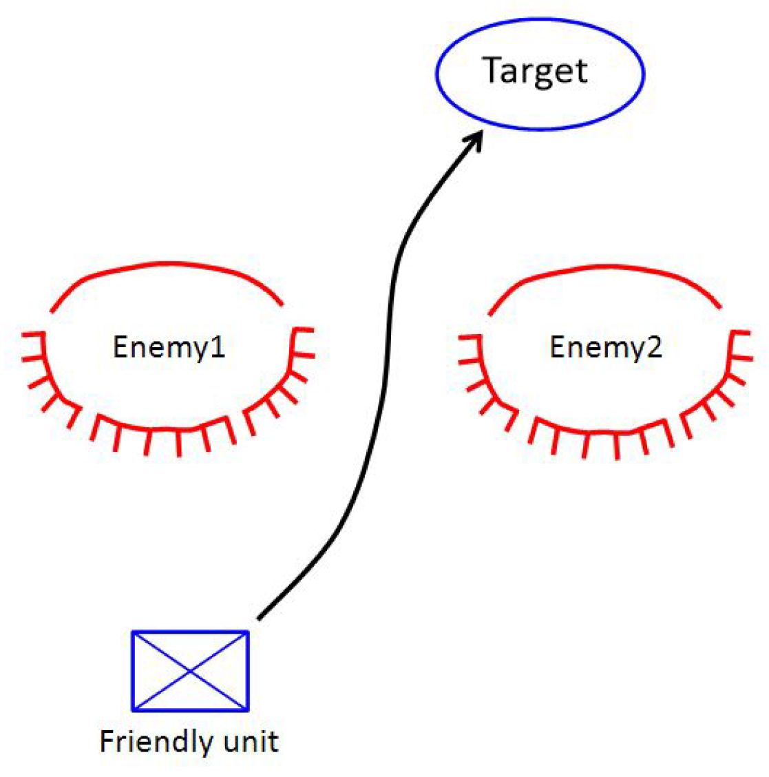
In the military context, path planning is important for unmanned weapons systems, which are gradually being developed and used on actual battlefields. Unmanned weapons systems such as UAVs (unmanned aerial vehicles) are not significantly affected by the environment because they operate in the air, above the terrain. However, UGVs are highly affected by the battlefield environment, which is uncertain and unpredictable. Since threats become obstacles on the battlefield [5], detection of the enemy’s position is very important, but the position obtained from prior information analysis continuously changes over time and is unpredictable. Additionally, since some threats, such as surveillance distance or rifle range, do not physically exist, it is difficult to implement these threats as obstacles. For these reasons, in some military operations, applying existing path-planning methods that provide pre-planned paths is not efficient. Exceptionally, if the prior information on the environment of a given battlefield is clear, there is no problem with applying the existing path-planning methods. However, since the ground battlefield environment of modern warfare changes rapidly, information analysis on the environment in which operations are conducted may not be sufficient. In order to overcome these battlefield characteristics, the Korean Ministry of National Defense is making efforts to develop MUM-T (manned-unmanned teaming), which is a new type of operation to achieve maximum efficiency by supplementing the shortcomings of manned and unmanned weapons systems. Recently, its utilization in ground forces is increasing. Based on this background, our study targets ground forces and assumes an operational situation in which a sudden enemy threat may occur in a continuously changing environment. In this case, algorithms applied to robots such as UGVs should not take up a lot of computational resources, so we designed a computationally cheap algorithm.
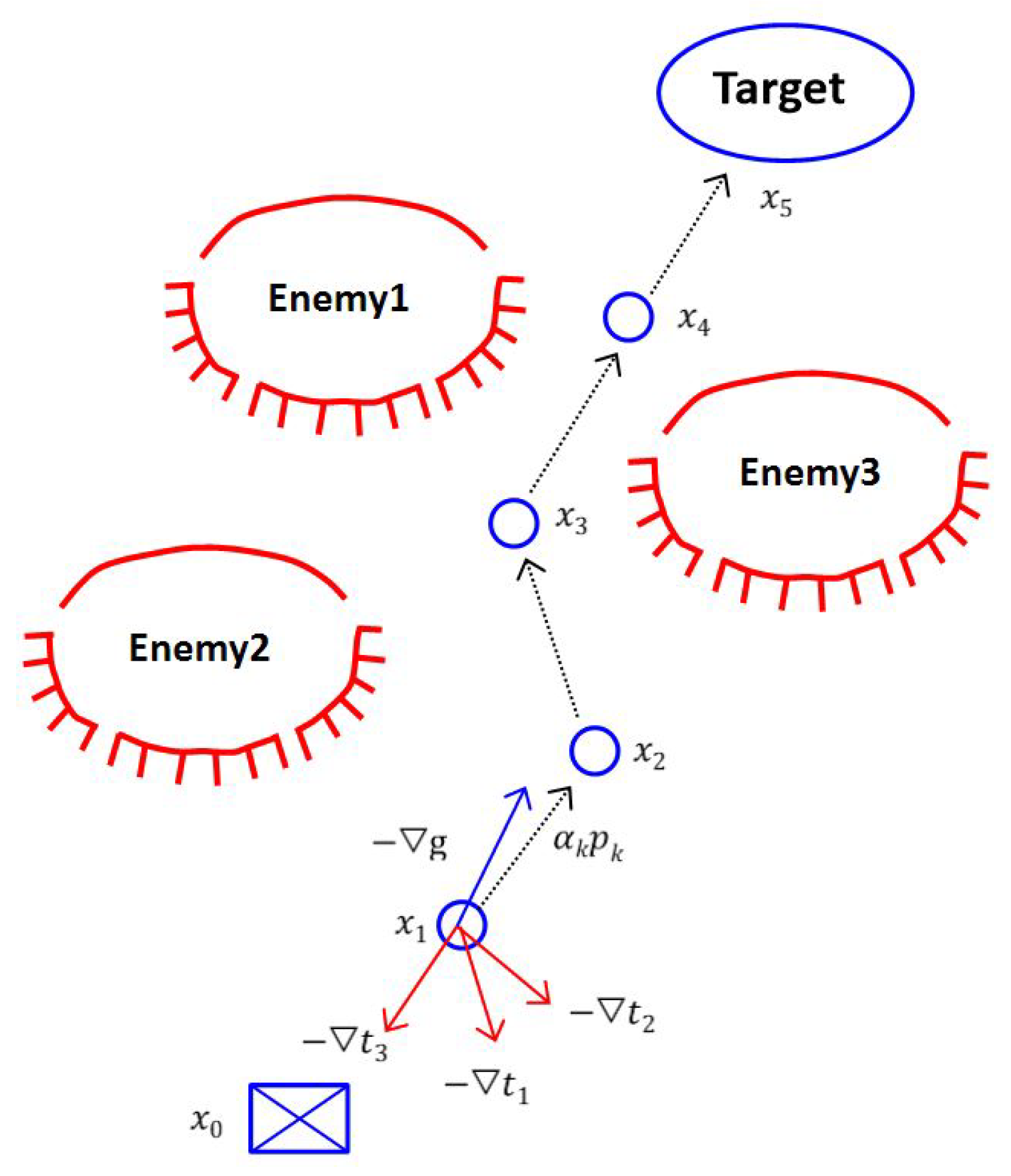
Our study presents a new path-planning algorithm that can be applied to the ground battlefield environment. The algorithm satisfies two conditions. First, it plans a path in near-real time, which enables a unit to respond quickly to changes on the battlefield. For example, if the enemy’s position changes during maneuvering due to ambush or concealment, our algorithm immediately finds a new path. Second, we implement enemy threats as obstacles by using a threat function. This function can change the size and shape of the enemy threat depending on the situation.
In Section 2, we introduce previous research on path planning. In Section 3, we describe the algorithmic path-planning sequence. We present the results obtained by applying the algorithm to sample models in Section 4 and conclude the research in Section 5.

2. Literature Review

Path planning is an optimization problem that plans an optimal path while avoiding collisions with obstacles. There are several common components that most path-planning studies consider. Although each study uses different terminology, the usual components are space, obstacles, and initial and goal states.
Space: The space can be an arbitrary two-dimensional space or a specific space such as a warehouse or a road. The space state allows for both discrete (finite or countably infinite) and continuous (uncountably infinite) states. The space definition is important because it affects both the design of the problem and the algorithm used.
Obstacles: Many studies focus on the implementation of obstacles, because this significantly affects the results of experiments. Obstacles can be an object, a wall, or in some cases a space that should not be accessed. The various shapes of obstacles are differently implemented according to the state space. In discrete space, the obstacles are simply expressed in a grid form [3]. In this case, a cost or probability is assigned to each cell to distinguish obstacles from spaces where a robot can move. In continuous space, obstacles can be expressed as various shapes, such as circles or curves [6].
Initial and goal state: Robots or vehicles have an initial point to start from and a goal point where the algorithm ends. In our study, the initial state is a start point, and the goal state is a target.
Depending on the specific definitions of the three components mentioned above, there are various methods of path planning. Among them, there are three representative path-planning methods, commonly distinguished in terms of space.
In discrete space, grid-based approaches, the most representative method set the space and obstacles with a grid [3]. This method is widely used and developed in various ways because it can easily configure the space, and such algorithms are well known for efficient path searching. That said, there are two major limitations that apply to situations where real-time path planning is required. First, prior information analysis of the given environment and obstacles is required, because it is necessary to decide at what interval the grid should be applied according to the size of the space and the shape of obstacles. The second is that as the space becomes larger or the grid becomes denser, the complexity of the problem increases rapidly and the computation time becomes longer [7]. Thus, most grid-based algorithms use heuristic methods [8] such as A* or D* algorithms, or ant colony optimization [3,9,10].
In continuous space, sampling-based approaches and potential-field approaches are typically used. Sampling-based approaches, such as rapidly-exploring random trees (RRTs) or probabilistic roadmaps, are used for stochastic searches [11]. These methods generate uniformly randomized direction or node samples and explore from start to end point [12]. RRTs and PRMs have been recognized as effective algorithms in high-dimensional spaces [13]. Nevertheless, as the size of space gets larger or obstacle shapes become more complex, the size of the sampled set increases [11].
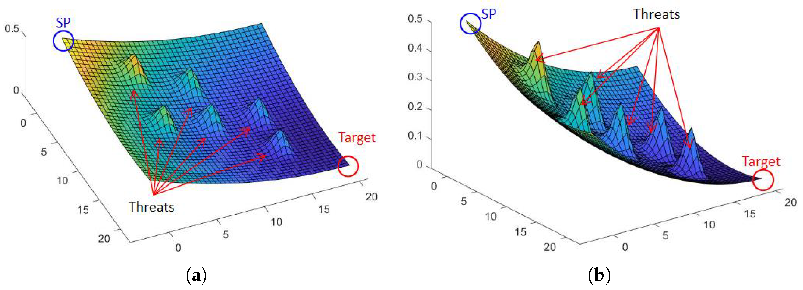
For potential-field-based approaches, Khatib and Oussama (1986) [14] suggested the concept of a potential field that consists of repulsive and attractive forces. Repulsive forces are used to avoid obstacles, and attractive forces are employed to reach the goal. These forces are implemented as functions. In this space, a robot moves autonomously due to forces without colliding with obstacles. This method is well known for real-time path planning, since it rapidly provides a local-minimum solution. However, this method has two typical problems. First, a local minimum trap can occur when a robot encounters a narrow passageway or multiple obstacles. Second, most studies have applied simple types of obstacles, such as circles [4] or walls. None of these studies showed a way to implement enemy threats which do not physically exist on the battlefield.
The uniqueness of our study derives from a review of the literature as follows:
  • We present a new path-planning algorithm that provides a path in near-real time reflecting the continuously changing environment.
  • To configure the environment, we define the potential field based on a penalty function.
  • We present a threat function that reflects the features of enemy threats on the battlefield.

3. Methodology

This section presents the problem definition considering the ground battlefield environment and suggests a new algorithm for planning a path.

3.1. Assumption

Our approach is based on the potential field method, with the field reflecting the battlefield environment. A two-dimensional continuous space is given in which a target exists as a goal to reach. Further, we assume the shapes of obstacles are defined as threats induced by the enemy’s defensive fighting position (DFP). A moving object—in other studies, usually a robot—is a friendly unit.
Figure 1 shows the concept of our approach’s configuration space with enemies, target, and a friendly unit. Even though the defensive position is shown as having already been set, we assume that a new enemy may suddenly appear or the existing DFP may change. Operationally, it is important to reach the target within the given time, so we focus not only on finding a collision-free path but also on determining the shortest of such paths.

3.2. PFP (Potential Field Based on Penalty Function) Model

The problem we define is to plan a path for friendly units to reach the target while avoiding enemy threats. We suggest the potential field based on a penalty function (hereafter referred to as PFP) model. In general, a penalty function is an objective function modified by reformulating a constraint as a penalty term in order to avoid straying too far from the feasible region [15]. The penalty function is defined as the sum of the threat function t j ( x ) with multiplier w j and the goal function g ( x ) with multiplier δ . The threat function acts in the potential field as a repulsive force that pushes a unit away from enemies, and the goal function acts as attractive force that pulls the unit toward the target.
Let the variable x be the coordinates of of the unit’s current position and j be an element in a set of threats T . Our PFP model is as follows.
min f ( x ) = j T w j t j ( x ) + δ g ( x )
We define the goal function g ( x ) as a penalty term whose value increases with the unit’s distance from the target. Specifically, we define g ( x ) as the 2-norm distance between x ^ (the target location) and x (current location of the unit) normalized by the distance between the start and end point. The definition of g ( x ) is as follows.
g ( x ) = x ^ x 2 x ^ x 0 2
To further discuss the PFP model’s procedure, we need to specify the threat function. Let t j ( x ) : R 2 R be a continuous and differentiable function of the enemy unit j’s position. t j ( x ) can be either convex or non-convex. In reviewing other literature in which the potential field is composed of functions to find the proper threat function, various functions have been applied to the potential field method. Kim et al. [16] configured a potential field by using a harmonic function. Figure 2 shows an example of a harmonic function’s surface plot. Hwang et al. [17] used a set of linear functions to implement the field of obstacles. Rasekhipour et al. [18] implemented triangular-shaped obstacles on the potential field.
However, these functions are not appropriate for our approach, because the threat function t j ( x ) is derived from the properties of enemy DFPs. For example, in a real battlefield, the threat increases as the unit gets closer to an enemy. Additionally, the shape of the threat induced by an enemy DFP is a distorted circle because the enemy defenses are oriented in a specific direction, rather than all directions uniformly: the threat is wide and gently sloping in the front, and narrow and steep in the rear. To satisfy these spatial features, we suggest an MSN (multivariate skewed-normal) distribution [19] as a threat function. The MSN distribution suggested by Azzalini and Dalla Valle (1996) takes the form
t ( x ) = 2 ϕ ( x ; σ 1 ) Φ ( α x ; σ 2 )
where ϕ and Φ denote the N ( 0 , 1 ) density and the distribution function, respectively. The parameters σ 1 and σ 2 are the standard deviations of density and distribution, and α is a given parameter. The details of this case will not be discussed in this paper. Instead, we suggest some parameters that determine the shape of the threat function. The parameters σ 1 and σ 2 are 2 × 2 matrices in which anti-diagonal elements are identical and determine the degree of distortion. The parameter α =   α 1 α 2 determines the position of distortion “position” which allows us to adjust the direction in which the enemy DFP is facing. Figure 3 shows the various shapes of enemy threats that changes according to these parameters.
Figure 4 shows an example of a PFP model’s surface plot. A descending slope is drawn across the plot from the start point to the target point. Threats are present In the field in the form of small mounds. The target is located at the lowest point of the potential field.

3.3. PFP Algorithm

Our approach is based on the line-search method. This method is generally applied on an unconstrained optimization model. The line-search procedure is as follows. First, at any point, a direction is searched by using first-order information for a given objective function. Second, the point moves one step to the next position by following the resulting direction. Third, this procedure is repeated until the point reaches a local minimum solution.
Figure 5 shows a conceptual diagram of our model. Red arrows are in opposite directions to threat function gradients, and the blue arrow is in the opposite direction to the gradient of the goal function. Black arrows are directions at the unit’s location determined as weighted sums of threat and goal vectors. Small blue circles connected by black arrows are current unit positions at the kth iteration, and the x k next to each blue circle represents its coordinates, where k { 0 , 1 , 2 , } . We define each x k as a sequence, and a set of sequences { x k } draws a path on the given space. Our primary interest in this study is not the local minimum solution x * , rather a set of sequences { x k } .
We next present the details of applying the line-search method. Let p k be a search direction where p k [ 1 , 1 ] × [ 1 , 1 ] . At any point x k , the next point is defined as x k + 1 = x k + α k p k , where the given parameter α k is the step length. We obtain first-order information by x f ( x ) :
f ( x k ) = j T w j t j ( x k ) + 2 δ k x ^ x 0 2 ( x ^ x k )
Since our objective function is a minimization problem, the direction p k needs to be a descent gradient. We choose the search direction at x k as
p k = f ( x k ) f ( x k )
Our approach is similar to descending a mountain efficiently. A climber searches direction based on the steepest slope at his position, proceeding down to the lowest point of the mountain while avoiding rocks or trees. Likewise, the friendly unit starts from the highest point of the potential field and moves step by step following the steepest descent gradient at each point to reach the lowest point of the field. The Algorithm 1 implementing this process is as follows.
Algorithm 1 PFP algorithm.
1:
Given: x ^ , t j ( x ) , δ k , j T , k K
2:
Initialization: x 0 = starting point, δ 0 = 0.08
3:
whilek = MAXITER or stop condition do
4:
    Calculate f ( x k ) = j T w j t j ( x k ) + δ k g ( x k )
      where, t j ( x k ) * t j ( x k ( 1 ) + ϵ ) t j ( x k ( 1 ) ) ϵ , t j ( x k ( 2 ) + ϵ ) t j ( x k ( 2 ) ) ϵ T , ( 0 < ϵ 1 e 10 )**
        where, x k ( 1 ) and x k ( 2 ) are x and y - coordinates of x k , respectively,
5:
    Calculate p k = f ( x k ) f ( x k )
6:
     x k + 1 x k + α k p k
6:
     where, α k 10 1 , 10 2 **
7:
     k k + 1
8:
    (If necessary) update δ k
9:
    Stop condition: x k x ^ 0.1
10:
end while
11:
Return sequence of x k as a path
* We approximate gradient of the threat function.
** Empirically chosen
This algorithm iterates the line-search method until the friendly unit reaches the target. In the iteration, we approximate the gradient of the threat function because the closed form of first order information of the MSN distribution is not known [19,20]. Additionally, we suggest α k and δ k empirically because the situation varies depending on the size of space and the number of enemy threats. The parameter δ k is important because it determines the size of the attractive force from the target. We describe the details for δ k in Section 4.

4. Computational Results

To verify the effectiveness of the algorithm proposed in this study, we experiment with various instances. The algorithm was coded in MATLAB (R2021b 9.11.0.1809720) and performed on an (Intel(R) Core(TM) i5-10210U CPU with 8 GB RAM.
We aimed to improve and check the algorithm in a simple instance consisting of a 10 × 10 space and two enemy threats. Additionally, we conducted several experiments to choose values for two parameters, δ k and α k , because these parameters significantly affect the path-planning result. Based on the experiments, we empirically chose δ k and α k that show the most stable result. Table 1 shows the simple instance and given parameters. The result in this instance is shown in Figure 6.
In Figure 6, the two contour plots (red lines) represent enemy threats. The blue line, drawn as a sequence of small dots, is a path. As we can see in Figure 6, we obtain a path that avoids enemy threats and reaches the target. Furthermore, it takes less than 2 s of computation time to obtain this result.
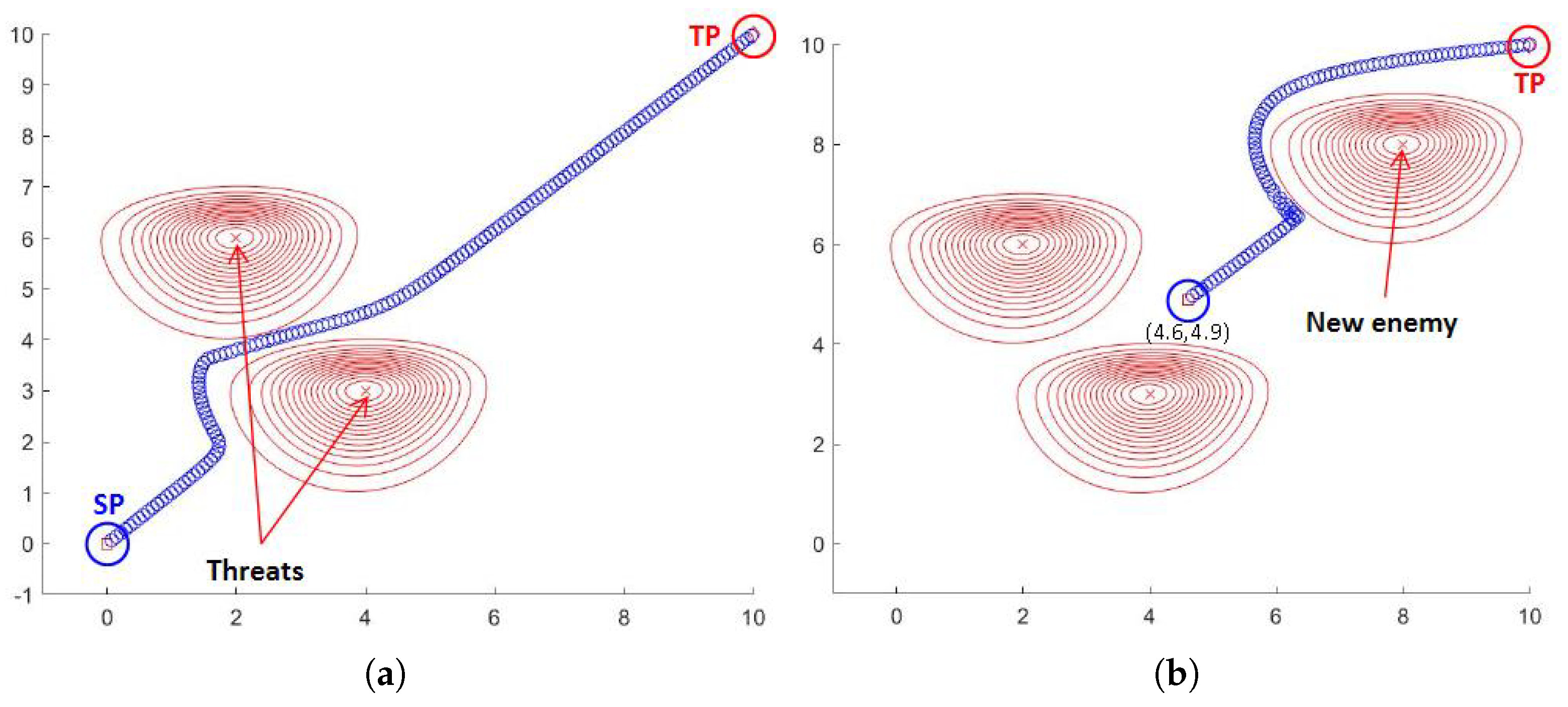
We now apply the algorithm to a larger-sized instance. The size of the space is 20 × 20, and the number of enemy threats is six. We conducted experiments in various environments, changing the positions of the start point, target, and enemy threats. Based on this experiment, it takes less than 5 s of computational time to plan a collision-free path. Figure 7 shows the results of the expanded experiments.
Additionally, we experimented to see if the algorithm works even in a changing environment. Contingency situations are likely to happen in military contexts and could affect another action or situation [21], such as ambush, concealment, or a situation caused by inaccurate prior information analysis. Hence, we create a situation in which an enemy suddenly appears while a unit is maneuvering toward the target.
Figure 8 shows the experimental results. The situation is as follows. At first, there are two enemies, and the expected path is shown in Figure 8a. We bring a new enemy when the unit reaches coordinates x k = ( 4.6 , 4.9 ) . In this situation, as shown in Figure 8b, the unit follows a modified path that is computed based on a new start point and the new enemy threat position. This process is repeated whenever information about the environment is updated.
The parameter δ k depends closely on both the threat function and the goal function. Figure 9 shows the different path-planning results according to the choice of δ k . These results show that the choice of δ k has a rule such that a large δ k causes the unit to ignore enemy threats, and a small δ k makes the unit move further away from enemy threats; if it is too small, the unit cannot reach the target. In Table 2 below, we suggest the appropriate δ k values that we empirically obtained in various sizes of space. Although we suggest empirical data for δ k , the choice of δ k can be flexible depending on the operational situation. For example, if a unit needs to reach a target as fast as possible, δ k needs to be increased. Conversely, if the purpose of an operation is to minimize vulnerability to enemy threats, δ k needs to be decreased.
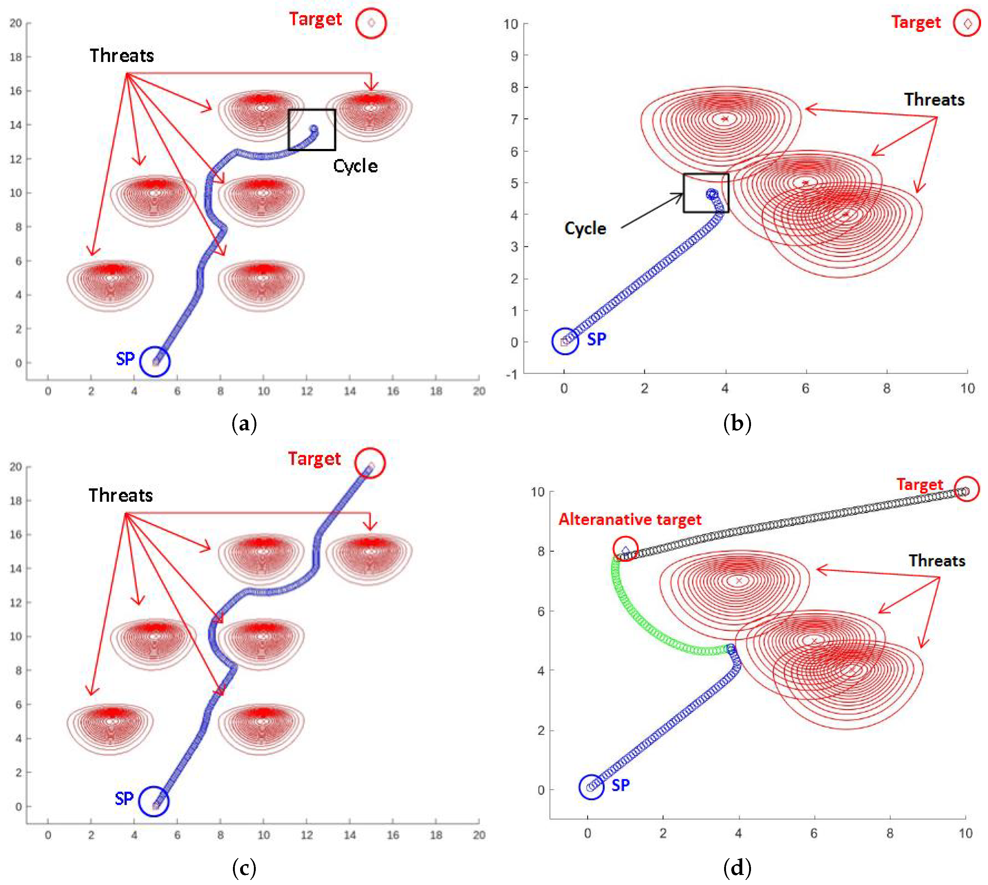
Even though the PFP algorithm performs efficiently and reaches the target in various conditions, we found a problem when changing the positions of the enemy threats and the size of the space. The problem is said to be a cycle [22], meaning that the sequence x k obtained by the algorithm converges to a specific point that is not the target point. There are two typical reasons that cause the cycling problem. First, a small δ k applied to an expanded space causes cycling because the distance between the start and target point affects the vector of the goal function, as described in Equation (2). Second, if the unit is surrounded or blocked by enemy threats, as shown in Figure 10, cycling can arise.
There are various empirical solutions to escape cycling. We suggest some of these. The simplest solution is to increase δ k , as shown in Figure 10c. Alternatively, input a random direction for a certain number of iterations, then return to the original algorithm or change direction p k toward an alternative target, such as a designated assembly point or an arbitrary point, as shown in Figure 10d. Although these empirical solutions are not always the best option because the way to escape cycling depends on the operational situation, they can nevertheless help to escape cycling in various situations.
We next discuss computational time, to verify the effectiveness of the algorithm. Table 3 shows various conditions and the results. The time gradually increases as the size of space becomes larger and the number of enemy threats increases. In our approach, the computation time in the table below is the sum of the time taken for each sequence. This means that, at any point, the time consumed by searching for direction and moving to the next position is shorter than that shown in the table. With this interpretation, robots or unmanned vehicles in the contingency situation that we described earlier do not need to wait for a new planned path. Rather, they continuously move to the next position by searching for a new direction in real time.

5. Conclusions

In this study, we presented a PFP model that provides a path for a friendly unit from a start point to a target while avoiding enemy threats. To develop the PFP model, we generated a potential field based on a penalty function in a two-dimensional space that reflects properties of the ground battlefield. Additionally, we described features of enemy threats induced by the enemy’s DFPs and suggested a threat function with an MSN distribution. Our experiments, described in Section 4, showed that the PFP model can obtain a path in near-real time. Additionally, as the size of the instance increases, our model has an increasing advantage in computation time because the algorithm only requires first-order information.
The findings regarding military perspectives derived from this study are as follows:
  • In the context of ground personnel forces such as special forces, conducting an infiltration—reaching the target without being detected by the enemy—is the most important operational task. The navigational equipment currently issued to the forces only provides a straight path to the target or a map graphic. Due to this limitation, accomplishing tasks depends on the commander’s ability to find a proper path. If the PFP model is applied to the equipment, it can suggest an appropriate direction considering both enemy threats and the target point. The commander can then maneuver to the target with less risk of exposure to enemy threats.
  • UGVs have been developed and are being used in ground battlefields. Their movement is mostly based on sensors or remote control. For example, unmanned reconnaissance vehicles follow a pre-planned path while avoiding obstacles detected by sensors. This system also requires remote control, since there is a possibility of losing a path if it deviates too much from the pre-planned path. The PFP algorithm is expected to overcome these limitations, allowing autonomous systems to develop further with technologies already in use. Additionally, adapting the algorithm to the system is not a huge burden, since the algorithm is computationally cheap, as mentioned above.
The PFP model has limitations in that the parameters are chosen empirically, and we applied a specific threat-function MSN distribution. Additionally, we assumed a two-dimensional continuous space for applying the algorithm on the ground battlefield. In view of these limitations, future research should define the parameters from a computational aspect. Additionally, based on literature reviewed in Section 2, for various obstacle functions in potential field-based studies, we can assume various shapes of threat and implement these as functions. In the context of military operations, research on other forms of induced threat from enemy operations besides DFP is also required. In terms of the dimension of space, since the same principle can be applied to our algorithm in a 3-dimensional space, it is required to study the application of the algorithm to a 3-dimensional space in consideration of the topographical effects of the ground battlefield.

Author Contributions

Conceptualization, N.C. and S.K.; methodology, N.S.; validation, N.C. and S.K.; formal analysis, N.S.; writing—original draft preparation, N.S.;writing—review and editing, N.C.; visualization, N.S.; supervision, N.C and S.K.; All authors have read and agreed to the published version of the manuscript.

Funding

This research received no external funding.

Data Availability Statement

Data sharing is not applicable to this article.

Conflicts of Interest

The authors declare no conflict of interest.

References

  1. Kumar, N.V.; Kumar, C.S. Development of collision free path planning algorithm for warehouse mobile robot. Procedia Comput. Sci. 2008, 133, 456–463. [Google Scholar] [CrossRef]
  2. Hu, X.; Chen, L.; Tang, B.; Cao, D.; He, H. Dynamic path planning for autonomous driving on various roads with avoidance of static and moving obstacles. Mech. Syst. Signal Process. 2018, 100, 482–500. [Google Scholar] [CrossRef]
  3. Šišlák, D.; Volf, P.; Pechoucek, M. Accelerated A* trajectory planning: Grid-based path planning comparison. In Proceedings of the 19th International Conference on Automated Planning & Scheduling (ICAPS), Thessaloniki, Greece, 19–23 September 2009; AAAI Press: Menlo Park, CA, USA, 2009; pp. 74–81. [Google Scholar]
  4. Iswanto, I.; Ma’arif, A.; Wahyunggoro, O.; Cahyadi, A.I. Artificial potential field algorithm implementation for quadrotor path planning. Int. J. Adv. Comput. Sci. Appl. 2019, 10, 575–585. [Google Scholar] [CrossRef] [Green Version]
  5. Bruvoll, S. Situation Dependent Path Planning for Computer Generated Forces; Norwegian Defence Research Establishment (FFI): Kjeller, Norway, 2014. [Google Scholar]
  6. Oroko, J.A.; Nyakoe, G.N. Obstacle avoidance and path planning schemes for autonomous navigation of a mobile robot: A review. In Proceedings of the Sustainable Research and Innovation Conference, Nairobi, Kenya, 12 November 2022; pp. 314–318. [Google Scholar]
  7. Krishnaswamy, G.; Stentz, A. Resolution Independent Grid-Based Path Planning; Carnegie-Mellon Univ Pittsburgh Pa Robotics Inst: Pittsburgh, PA, USA, 1995. [Google Scholar]
  8. Karur, K.; Sharma, N.; Dharmatti, C.; Siegel, J.E. A survey of path planning algorithms for mobile robots. Vehicles 2021, 3, 448–468. [Google Scholar] [CrossRef]
  9. Stentz, A. Optimal and efficient path planning for partially known environments. In Intelligent Unmanned Ground Vehicles; Springer: Boston, MA, USA, 1997; pp. 203–220. [Google Scholar]
  10. Ajeil, F.H.; Ibraheem, I.K.; Azar, A.T.; Humaidi, A.J. Grid-based mobile robot path planning using aging-based ant colony optimization algorithm in static and dynamic environments. Sensors 2020, 20, 1880. [Google Scholar] [CrossRef] [PubMed] [Green Version]
  11. Gammell, J.D.; Srinivasa, S.S.; Barfoot, T.D. Informed RRT*: Optimal sampling-based path planning focused via direct sampling of an admissible ellipsoidal heuristic. In Proceedings of the 2014 IEEE/RSJ International Conference on Intelligent Robots and Systems, Chicago, IL, USA, 14–18 September 2014; pp. 2997–3004. [Google Scholar]
  12. LaValle, S.M. Planning Algorithms; Cambridge University Press: Cambridge, UK, 2006. [Google Scholar]
  13. Devaurs, D.; Siméon, T.; Cortés, J. Optimal path planning in complex cost spaces with sampling-based algorithms. IEEE Trans. Autom. Sci. Eng. 2015, 13, 415–424. [Google Scholar] [CrossRef] [Green Version]
  14. Khatib, O. Real-time obstacle avoidance for manipulators and mobile robots. In Proceedings of the 1985 IEEE International Conference on Robotics and Automation, St. Louis, MO, USA, 25–28 March 1985; pp. 500–505. [Google Scholar]
  15. Smith, A.E.; Coit, D.W.; Baeck, T.; Fogel, D.; Michalewicz, Z. Penalty functions. In Handbook of Evolutionary Computation; IOP Publishing Ltd.: Bristol, UK, 1997; Volume 97, p. C5. [Google Scholar]
  16. Kim, J.O.; Khosla, P. Real-Time Obstacle Avoidance Using Harmonic Potential Functions. IEEE Trans. Robot. Autom. 1992, 8, 338–349. [Google Scholar] [CrossRef] [Green Version]
  17. Hwang, Y.K.; Ahuja, N. A potential field approach to path planning. IEEE Trans. Robot. Autom. 1992, 8, 23–32. [Google Scholar] [CrossRef] [Green Version]
  18. Rasekhipour, Y.; Khajepour, A.; Chen, S.K.; Litkouhi, B. A potential field-based model predictive path-planning controller for autonomous road vehicles. IEEE Trans. Intell. Transp. Syst. 2016, 18, 1255–1267. [Google Scholar] [CrossRef]
  19. Azzalini, A.; Valle, A.D. The multivariate skew-normal distribution. Biometrika 1996, 83, 715–726. [Google Scholar] [CrossRef]
  20. Wright, S.; Nocedal, J. (Eds.) Numerical Optimization; Springer: New York, NY, USA, 1999. [Google Scholar]
  21. Bowyer, R. Dictionary of Military Terms; Routledge: London, UK, 2018. [Google Scholar]
  22. Lumelsky, V.; Stepanov, A. Dynamic path planning for a mobile automaton with limited information on the environment. IEEE Trans. Autom. Control 1986, 31, 1058–1063. [Google Scholar] [CrossRef]
Figure 1. An example of a conceptual diagram of our approach.
Computation 11 00012 g001
Figure 2. An example of a harmoric function’s surface plot.
Computation 11 00012 g002
Figure 3. Various threat function shapes by MSN distribution: (a) basic shape; (b) changing the degree of distortion; (c) changing direction toward the south; (d) changing direction toward the northwest.
Computation 11 00012 g003
Figure 4. Example of the PFP model’s 3D surface plot: (a) 3D surface plot viewed from above; (b) 3D surface plot viewed from side.
Computation 11 00012 g004
Figure 5. Sample conceptual diagram of a PFP model.
Computation 11 00012 g005
Figure 6. Path planning result for a simple instance experiment.
Computation 11 00012 g006
Figure 7. Path planning results in large instances: (a) Initial state of expanded instance. (b) Changing the start and target point. (c) Changing enemy threat positions. (d) Changing all components.
Computation 11 00012 g007
Figure 8. Path planning in a contingency situation: (a) initial state with two enemy threats; (b) contingency situation: a new enemy appears.
Computation 11 00012 g008
Figure 9. Effect on the path planning of choice of δ k : (a) result when δ k is large ( δ k = 2 ); (b) result when δ k is small ( δ k = 0.01 ).
Computation 11 00012 g009
Figure 10. Cycling problems and remedies: (a) Cycling caused by inappropriate δ k . (b) Cycling caused by enemy threats. (c) Remedy for problem (a): changing δ k ; (d) remedy for problem (b): changing direction p k to an intermediate point.
Computation 11 00012 g010
Table 1. Simple instance and parameters.
MAXITERStart PointTargetEnemy Position δ k α k
K = 300 x 0 = (0, 0) x ^ = (10, 10)Enemy 1 = (4, 6)
Enemy 2 = (7, 3)
0.080.1
Table 2. The suggested range of δ k that was empirically obtained.
Size of Space x ^ x 0 2 The Suggested Range of δ k
10 × 102000.08 ≤ δ k ≤ 0.2
20 × 204000.3 ≤ δ k ≤ 0.5
30 × 3018000.7 ≤ δ k ≤ 0.9
Table 3. Computational time of the PFP model in various conditions.
MAXITERSize of SpaceNumber of
Enemy Threats
δ k α k Computation
Time(s)
30010 × 1020.080.11.760
42.609
20 × 2040.30.22.931
63.832
30 × 3060.70.35.117
85.488
50010 × 1020.080.12.273
43.421
20 × 2040.30.23.642
64.679
30 × 3060.70.35.329
86.909
100010 × 1020.080.13.306
44.918
20 × 2040.30.25.087
66.760
30 × 3060.70.38.171
811.302
Disclaimer/Publisher’s Note: The statements, opinions and data contained in all publications are solely those of the individual author(s) and contributor(s) and not of MDPI and/or the editor(s). MDPI and/or the editor(s) disclaim responsibility for any injury to people or property resulting from any ideas, methods, instructions or products referred to in the content.

