Credit Spreads, Leverage and Volatility: A Cointegration Approach

Abstract

This work documents the existence of a cointegration relationship between credit spreads, leverage and equity volatility for a large set of US companies. It is shown that accounting for the long-run equilibrium dynamic between these variables is essential to correctly explain credit spread changes. Using a novel structural model in which equity is modeled as a compound option on the firm’s assets, a new methodology for estimating the unobservable market value of the firm’s assets and volatility is developed. The proposed model allows to significantly reduce the pricing errors in predicting credit spreads when compared with several structural models. In terms of correlation analysis, it is shown that not accounting for the long-run equilibrium equation embedded in an error correction mechanism (ECM) results into a misspecification problem when regressing a set of explanatory variables onto the spread changes. Once credit spreads, leverage and volatility are correctly modeled, thus allowing for a long-run equilibrium, the fit of the regressions sensibly increases if compared to the results of previous research. It is further shown that most of the cross-sectional variation of the spreads appears to be more driven by firm-specific characteristics rather than systematic factors.

1. Introduction

Structural models of credit risk have faced several difficulties in explaining both the level and changes of bond and CDS spreads observed in the data since its pioneering introduction by [1]. The early empirical work by [2] shows that the Merton model for callable coupon bonds overprices such bonds. This findings have motivated a variety of extensions, such as allowing for default before the bond maturity, stochastic interest rates, jumps, and strategic default. Despite these extensions, the structural approach is still questioned regarding its ability to explain the level of credit spreads ([3]).

This work attempts at giving an alternative explanation to the (alleged) lack of accuracy by structural models of default to explain credit spreads. In particular, the most important finding of the paper is that the documented inability by such models to describe both the cross-section and the time-series components of the spreads lies first in the type of default model chosen for the analysis, but mostly in the econometric tools employed for assessing the goodness to fit of the former.

Given the recent findings in [4] documenting the need of a time-varying volatility of the asset in order to explain the level of credit spread over medium- and long-term maturities, a novel estimation technique of a time-varying volatility of the assets is introduced herein. However, the novel structural model proposed here as well as the related estimation technique are much simpler than the one in [4]. As a matter of fact, their calibration methodology relies on the Fortet’s lemma, maximum likelihood and Chebychev interpolation in the case of stochastic diffusive asset volatility (and, on top of those, on simulated maximum likelihood when jumps are introduced). They have 9 parameters, over a total of 12, to estimate. In this paper, even though the asset value process is assumed to follow a geometric Brownian motion (thus asset volatility is not stochastic), the proposed estimation methodology allows to retrace the time series of the asset volatility for a given firm. Hence, the time series of the equity volatility can be also estimated accordingly.

To help the reader navigate throughout the paper, a brief roadmap of the steps and findings is provided:

(a)

A new structural model is developed along the lines of [1,5]. The model developed here is an extension of the Merton’s model in which the firm’s equity is priced as an n-fold compound call option instead of a vanilla call option; this allows to account for more than one debt maturing at only one future date, which surely is one of the most evident limitations of the Merton’s model.

(b)

A new estimation technique is implemented for those variables which structural models of default predict to be the drivers for the spreads. More specifically, a simple estimation which relies only on the joint calibration on the price of the equity and CDS spreads (and, indirectly, by the book value of the firm’s debt) is proposed to estimate the value of the firm’s assets alongside its volatility, which are both unobservable quantities.

(c)

Once the asset volatility and the market leverage are estimated, the goodness of these estimates is tested as their own ability to predict the one-period ahead CDS spreads. Different combinations of the model parameters are tested in order to obtain a satisfying calibration.

(d)

Finally, an econometric analysis of the determinants of the credit spreads is conducted using an error correction mechanism (ECM).

The findings in (d) are the most interesting, as, to the best of my knowledge, the  inability of structural models to explain the level of credit spreads has never been addressed via cointegration analysis. In fact, previous works such as [6,7,8,9] investigated the link between credit spreads and their determinants via simple linear regressions. There, a set of variables (usually leverage, equity volatility and characteristics of the term structure of interest rates) is regressed onto the spreads in order to explain their level and changes. This paper shows that use of such regressions to explain the level of the spreads (either bonds or CDS) is intrinsically flawed. As shown later in the paper, the level of credit spreads, as well as other variables entering the regressions, display a unit root. Therefore, any regression analysis based on these variables would detect spurious correlations. Hence, the only consistent way to tackle this problem is investigating the presence of a long-run equilibrium equation between these variables using an error correction mechanism (ECM), as introduced by [10]. If these variables are cointegrated (that is, if there exists a linear combination of them which is stationary), an ECM can be estimated and the economic relationship between them can be further investigated. If the variables are not cointegrated, only the changes in spreads can be explained by regressing the first differences those variables onto the former (alternatively, a stationary VAR can be used). The use of an ECM, when possible, is more desirable, as it allows to shed light on the economic, and not only statistical, relationship between the variables.

It still appears surprising how previous works fully ignore a possible cointegration, despite [11] developing a VECM to investigate the cointegration of bond and CDS spreads. Such analysis is possible only if the time-series component of the spreads is non-stationary. Here, instead, a cointegration analysis is conducted between the CDS spreads and their determinants as predicted by the structural models of default. This leads to a cointegrated system, where credit spreads, financial leverage and the firm’s riskiness comove, adjusting to a long-run equilibrium. Empirical results discussed in this paper support the existence of a cointegrating relationship between these variables

In the following analysis, CDS rather than bond spreads are used, as the former constitute a more direct and clean signal for the underlying default risk. In fact, CDS spreads provide relatively pure pricing of the default event of the underlying entity, as they are typically traded on standardized terms. In fact, unlike bonds, CDSs have a constant maturity, the underlying instrument is always par valued, they concentrate liquidity in one instrument, and are not affected by different taxation regimes; also, bond spreads are more likely to be affected by differences in contractual arrangements, such as differences in seniority, coupon rates, embedded options, and guarantees. Secondly, many corporate bonds are bought by investors who simply hold them to maturity, and the secondary market liquidity is therefore often poor. Furthermore, shorting bonds is even more difficult in the cash market, as the repo market for corporate bond is often illiquid, and the tenor of the agreement is usually very short. CDS contracts instead allow investors to implement trading strategies to hedge credit risk over a longer period of time at a known cost. Moreover, as shown by [11], CDS spreads tend to respond more quickly than bond spreads to changes in credit conditions in the short run.

The rest of the paper is organized as follows. Section 2 provides a short literature review of the works connected to the paper. Section 3 introduces the compound option structural model of default alongside the estimation methodology for the firm’s asset value and volatility. Section 4 models the cointegration relationship between the variables, and the short-term adjustment is estimated. Finally, Section 5 discusses the main findings and performs some robustness checks. Section 6 concludes.

2. Literature Review

Academic research has taken mainly three routes in analyzing the quite surprising lack of accuracy of structural models in explaining the observed credit spreads.

Firstly, attempts to empirically implement models on individual corporate bond spreads have failed ([12]). Mixed evidence supporting the structural approach is instead documented for CDS spreads ([8,9]), thus suggesting liquidity and tax arguments for the lack of success in case of bonds ([13,14]). Ref. [15] finds that expected losses account for a low fraction of spreads for investment grade bonds. Ref. [6] documents that proxies for credit risk explain only a small portion of changes in yield spreads and that the unexplained portion is driven mainly by factors that are independent of both credit-risk and standard liquidity measures.

Secondly, efforts to calibrate models to observable moments, including historical default rates and Sharpe ratios, have been unable to match average credit spreads levels (the so-called credit spread puzzle). Ref. [3], testing over an extensive class of structural models, shows that credit risk accounts for only a small fraction of yield spreads for investment-grade bonds of all maturities, with the fraction lower for bonds of shorter maturities, but it accounts for a much higher fraction of yield spreads for high-yield bonds. They calibrate each of the models on the historical default loss experienced and equity risk premia, and demonstrate that different models (under)predict similar credit risk premia.

Thirdly, models have been unable to jointly explain the dynamics of credit spreads and equity volatilities. Within this framework of research, ref. [16] finds that idiosyncratic volatility can explain one-third of yield spreads for investment grade bonds rated below Aaa. An important recent development which examines potential links between the credit spread puzzle and macroeconomic conditions using consumption-based asset-pricing is [17]. The authors show that the [18] pricing kernel combined with some mechanism to match the countercyclical nature of defaults is able to capture the level and time variation of Baa-Aaa spreads. However, they also show that a pricing kernel that explains the equity premium with a constant Sharpe ratio cannot explain the credit spread.

A recent paper which tries to address all the above-mentioned failures of structural models of default in explaining credit spreads is [4]. In their paper, the authors use the framework in [19] (i.e., the firm has issued a consol bond) in which the unlevered asset process is modeled as in [20]. Thus allowing for stochastic volatility in firm value process and calibrating the variance risk premium consistently with reasonable firm-level Sharpe ratios, they are first able to resolve the credit spread puzzle for medium- to longer-term maturities for representative Baa- and Aa-rated firms. Secondly, introducing jumps in the asset value process allows to fit shorter term credit spreads as well. Moreover, their model succeeds at explaining the joint dynamics of credit spreads and equity volatilities, and allows them to identify economically significant variance risk premia, which explain an important part of spread levels.

To summarize, this works hopes to fill some theoretical, methodological and empirical gaps detected in this literature, more specifically, the following:

• Provide a novel and richer, though still tractable, structural model of default which removes one of the most stringent restriction of the Merton’s model, namely clustering the firm’s debt at one single point in time (theoretical);
• Develop a new estimation technique for some crucial unobservable variables, such as the value of the firm’s assets and volatility (methodological);
• Conduct a cointegration analysis on a large panel of US CDS spreads (using the estimated variables) to show that large part of the empirical failure of structural models is more apparent than real as it was largely due to an omitted variable problem (empirical).

3. The Model, Estimation Methodology and Data Description

3.1. The Compound Option Model

Consider a firm which has issued n bonds and equity, both receiving payments in the form of coupons and dividends. According to the indenture of the bonds: (1) the firm promises to repay each bond, with face value $F_i$, to the bondholders at known times $t_i\in (t_0,t_n]$, $i\in I:=\left\{1,\dots ,n\right\}$; (2) in case of default, which may occur only at the given $t_i$s, the bondholders immediately take over the company, and the shareholders receive nothing; and (3) the firm cannot issue any senior or equivalent rank claims on the firm nor do share repurchases before $t_n$. Usual assumptions in terms of transaction cost, taxes, bid/ask spreads, short-selling and indivisibility of assets apply.

For convenience of notation, set $t_0:=0$ and denote the generic payoff at time $t_i$ as $X_{t_i}:=X_i$. Let V, S and D represent the firm’s assets, equity and debt, respectively. According to the structural approach and the Modigliani–Miller theorem, both equity and debt are functions of the firm’s assets and not vice versa ([21]). It is important to have in mind that under the structural approach to default, there is one state variable, namely V, which drives the prices of all the assets in the economy: both S and D (and any derivatives written on them) are functions of V and, of course, of the parameters driving the process assumed for V. Neither S nor D can be functions of one another; this would violate the Modigliani–Miller Proposition I (with no taxes).

Then, fix a filtered probability space $(\Omega ,\mathcal{F},\mathbb{F},\mathbb{P})$ and assume no-arbitrage conditions in the economy. Under certain technical conditions, there exists a risk-neutral probability measure $\mathbb{Q}$, equivalent to $\mathbb{P}$ such that the gain process associated with any admissible trading strategy deflated by the risk-free rate is a martingale. Furthermore, the following notation for the (risk-free) discount factor

$$\mathrm{DF}(t_i,t_j)=\frac{B_i}{B_j}=exp\left(-{\int }_{t_i}^{t_j}{r}_s\mathsf{d}s\right),$$

is used, being that $B_t=exp\left({\int }_0^t{r}_s\mathsf{d}s\right)$ is the value of the money-market account at time t, and $r_t$ is a (possibly stochastic) positive function of time.

Similarly to [5], the firm refinances each bond payment with equity. In this setting, bankruptcy occurs when the firm fails to make the reimbursement payment because it is unable to issue new equity. Ref. [22] argues that the firm will find no takers for its stock whenever the value of the equity, if the payment is made, is less than the value of the payment due. If all of the firm debt is finally repaid, the firm is liquidated, and the shareholders receive any remaining value as a lump-sum liquidating dividend.

More specifically, if at time $t_i$ the value of equity prior to making the payment is larger than payment due, the bond is paid off and the firm is kept alive; otherwise, bondholders declare bankruptcy. In the case that the bond is repaid, the same mechanism occurs at the next payment date, $t_{i+1}$, and so on until the last payment date, $t_n$. This mechanism can also be interpreted as the firm defaulting on its debt because is unable to issue new equity ([5]). Hence, the default time is defined as

$$\tau :=\underset{i\in I}{inf}\left\{t_i:S_i^{\star }\left(V\right)<F_i\right\}$$

(1)

where $S_i^{\star }\left(V\right)$ is the continuation value of equity, that is the value of equity before paying the bond, e.g., if the continuation value of the equity $S^{\star }$ is 20 and the face value of debt is 30, then equity is worthless ($S=0$). The eventuality that shareholders may have an incentive to raise new equity to keep receiving dividends in the future, thus postponing default, is not possible within this model. Most importantly, though the process driving both the firm’s assets and equity will be assumed to be defined in continuous time, default is assumed to occur only at discrete times, namely when the bonds outstanding are due. This is clearly a limitation and main feature of compound option model of default. For structural models in which the default barrier is monitored continuously, see, among others, ref. [19,22,23].

As for any structural model, given that the firm’s equity is a function of the firm value, default times can be re-expressed as events in the asset value space: for each value of equity which triggers default corresponds only one value of the firm assets, namely ${\overline{V}}_i$ at time $t_i$, which implies (1), that is

$$\tau =\underset{i\in I}{inf}\left\{t_i:V_i<{\overline{V}}_i\right\}.$$

The default barrier ${\left({\overline{V}}_i\right)}_{i\in I}$ can be interpreted as a latent sequence of thresholds embedded into the firm’s capital structure and riskiness. Operationally, the default thresholds are found recursively starting from the default threshold in $t_n$, which coincides with $F_n$ as in the Merton’s model. The other values of the barrier are calculated as the solution of an integral equation, where the dimension of the integrals increases alongside with the number of bond outstanding (i.e., given n bond outstanding, $n-1$ integral equation must be solved, being the last integral to be solved an $(n-1)$-dimensional integral).

Within this framework, both the present and the continuation value of the equity can be calculated as the risk-neutral expectation of their terminal payoffs. At any time $t_i\in [0,t_n]$, the terminal payoff of the the firm’s equity can be expressed as

$$S_n\left(V\right)=V_n{𝟙}_{\tau >t_n}-\sum _{k=i+1}^n\frac{F_k}{\mathrm{DF}\left(t_k,t_n\right)}{𝟙}_{\tau >t_k}.$$

The interpretation of the payoff function is straightforward: equity holders receive the asset value in $t_n$ (if the firm has been able to repay all its outstanding debt), net of all the future reimbursements (if the firm has survived at each default point).

The continuation value of the equity is given by the present value of the expected payoff of the equity before having checked for the potential default occurring at $t_i$, that is

$$\begin{array}{cc}\hfill S_i^{\star }\left(V\right)& ={\mathbb{E}}_i^{\mathbb{Q}}\left[\mathrm{DF}\left(t_i,t_n\right)S_n\left(V\right)\right],\hfill \end{array}$$

(2)

where the ${\mathbb{E}}_i^{\mathbb{Q}}(·)\equiv {\mathbb{E}}^{\mathbb{Q}}(·|{\mathcal{F}}_{t_i})$. As a consequence, the value of the equity is given by

$$S_i\left(V\right)=max\left\{S_i^{\star }\left(V\right)-F_i,0\right\}.$$

See Figure 1 for a visual representation of the continuation and actual value of the equity. Under (1) and (2), it can be further expressed in terms of events in equity space and, ultimately, in the asset value space. Therefore, we have the following.

$$\begin{array}{cc}\hfill S_i^{\star }\left(V\right)& ={\mathbb{E}}_i^{\mathbb{Q}}\left(\mathrm{DF}\left(t_i,t_n\right)V_n{𝟙}_{{\bigcap }_{h=i+1}^n\left\{S_h^{\star }\left(V\right)\ge F_h\right\}}\right)-\sum _{k=i+1}^n{F}_k{\mathbb{E}}_i^{\mathbb{Q}}\left(\mathrm{DF}\left(t_i,t_k\right){𝟙}_{{\bigcap }_{h=i+1}^k\left\{S_h^{\star }\left(V\right)\ge F_h\right\}}\right)\hfill \\ \hfill & ={\mathbb{E}}_i^{\mathbb{Q}}\left(\mathrm{DF}\left(t_i,t_n\right)V_n{𝟙}_{{\bigcap }_{h=i+1}^n\left\{V_h\ge {\overline{V}}_h\right\}}\right)-\sum _{k=i+1}^n{F}_k{\mathbb{E}}_i^{\mathbb{Q}}\left(\mathrm{DF}\left(t_i,t_k\right){𝟙}_{{\bigcap }_{h=i+1}^k\left\{V_h\ge {\overline{V}}_h\right\}}\right).\hfill \end{array}$$

(3)

Notice that (3) is the most general expression for the continuation value of the equity. So far, no distributional assumptions have been made on the process driving the asset value nor on the form of the discount factor. The asset value process could be a Lévy process, as well as a process with continuous paths and stochastic volatility; similarly, the discount factor could be assumed stochastic. However, ref. [24] shows that compound option problems, such as in [5,25,26], can neither be solved in a semi-closed form under stochastic interest rates nor stochastic volatility. Consequently, in order to preserve analytical tractability, a positive constant continuously compounded risk-free rate r is assumed throughout. Additionally, a geometric Brownian motion is considered for the asset value process, that is

$$\mathsf{d}{V}_t=\left(r-p\right)V_t\mathsf{d}t+{\sigma }_V{V}_t\mathsf{d}{W}_t^{\mathbb{Q}},$$

(4)

where p is the continuously compounded payout rate, ${\sigma }_V$ the instantaneous volatility of the assets, and $W_t^{\mathbb{Q}}$ a $\mathbb{Q}$-standard Brownian motion. The asset value is modeled as a geometric Brownian motion, as it allows to obtain semi-closed formulas for the compound option problem.

Defining the events ${\mathcal{V}}_{i,k}:={\bigcap }_{h=i+1}^k\left\{V_h\ge {\overline{V}}_h\right\}$, the $t_i$-continuation value of the equity can be written as

$$S_i^{\star }\left(V\right)=e^{-r\left(t_n-t_i\right)}{\mathbb{E}}_i^{\mathbb{Q}}\left(V_n{𝟙}_{{\mathcal{V}}_{i,n}}\right)-\sum _{k=i+1}^n{e}^{-r\left(t_k-t_i\right)}{F}_k{\mathbb{E}}_i^{\mathbb{Q}}\left({𝟙}_{{\mathcal{V}}_{i,k}}\right),$$

(5)

and for $t_i=t_0$, it follows

$$\begin{array}{cc}\hfill S_0\left(V\right)& =e^{-r{t}_n}{\mathbb{E}}^{\mathbb{Q}}\left(V_n{𝟙}_{{\mathcal{V}}_n}\right)-\sum _{k=1}^n{e}^{-r{t}_k}{F}_k\mathbb{Q}\left({\mathcal{V}}_k\right),\hfill \end{array}$$

(6)

where ${\mathcal{V}}_k\equiv {\mathcal{V}}_{0,k}$, for $k\in I$. Notice that the $t_0$-continuation value of the equity and the contemporaneous value of the equity coincide as no debt is due in $t_0$ (i.e., $F_0=0$). In order to derive an analytical solution, a change of measure as in [26] is performed such that $\widehat{\mathbb{Q}}\sim \mathbb{Q}$, with 

$${\left.\frac{\mathsf{d}\widehat{\mathbb{Q}}}{\mathsf{d}\mathbb{Q}}\right|}_{{\mathcal{F}}_t}=\frac{V_t{e}^{pt}}{V_0{B}_t}=exp\left({\sigma }_V{W}_t^{\mathbb{Q}}-\frac{{\sigma }_V^2}{2}t\right).$$

The measure $\widehat{\mathbb{Q}}$ is referred as the firm-value fund measure thereafter. Setting $t=t_n$, it follows

$$\begin{array}{c}\hfill S_0\left(V\right)=e^{-p{t}_n}{V}_0\widehat{\mathbb{Q}}\left({\mathcal{V}}_n\right)-\sum _{k=1}^n{e}^{-r{t}_k}{F}_k\mathbb{Q}\left({\mathcal{V}}_k\right).\end{array}$$

In order to compute the probabilities under $\mathbb{Q}$ and $\widehat{\mathbb{Q}}$, the result about multivariate Gaussian probabilities in [5] is used. Hence, the two probabilities can expressed as the following multivariate Gaussian integrals:

$$\begin{array}{cc}\hfill S_0\left(V\right)& =e^{-p{t}_n}{V}_0{\Phi }_n\left({\mathbf{d}}^{+};{\mathbf{\Gamma }}_n\right)-\sum _{k=1}^n{e}^{-r{t}_k}{F}_k{\Phi }_k\left({\mathbf{d}}_k^{-};{\mathbf{\Gamma }}_k\right)\hfill \end{array}$$

(7)

where ${\mathbf{d}}^{+}:={\left(d_i^{+}\right)}_{1\le i\le n}$ and ${\mathbf{d}}_k^{-}={\left(d_i^{+}-{\sigma }_V\sqrt{t_i}\right)}_{1\le i\le k}$ with

$$d_i^{+}=\frac{ln\left(V_0/{\overline{V}}_i\right)+\left(r-p+{\sigma }_V^2/2\right)t_i}{{\sigma }_V\sqrt{t_i}},{\mathbf{\Gamma }}_k=\left(\begin{array}{ccccc}1& \sqrt{\frac{t_1}{t_2}}& \sqrt{\frac{t_1}{t_3}}& \dots & \sqrt{\frac{t_1}{t_k}}\\ & 1& \sqrt{\frac{t_2}{t_3}}& \dots & \sqrt{\frac{t_2}{t_k}}\\ \dots & \dots & \dots & \dots & \dots \\ & & & 1& \sqrt{\frac{t_{k-1}}{t_k}}\\ & & & & 1\end{array}\right).$$

and ${\Phi }_i(\mathbf{z};\mathbf{\Gamma })$ is the cumulative distribution function of an i-dimensional normal random vector with zero mean and covariance matrix $\mathbf{\Gamma }$ calculated over the set ${╳}_{j=1}^i(-\infty ,z_j)$. Notice that, if $n=1$ and $p=0$, the model coincides with the Merton’s model.

3.2. Estimation of the Unobservable Asset Value and Volatility

The unobservable parameters of the model are the value of the firm assets, V, and the asset volatility, ${\sigma }_V$. As the sequence of risk-neutral probabilities $\mathbb{Q}\left(\tau \ge t_i\right)$ can be estimated from the CDS spreads in a model-free fashion as in [27], the following system of non-linear equations can be employed to estimate both variables:

$$\left\{\begin{array}{c}S\left(V,{\sigma }_V\right)=S\hfill \\ {\Phi }_i^{-}(V,{\sigma }_V)=\mathbb{Q}\left(\tau \ge t_i\right)\forall i\in I.\hfill \end{array}\right.$$

(8)

Here, the functional form of $S\left(V,{\sigma }_V\right)$ and ${\Phi }_i^{-}(V,{\sigma }_V)={\Phi }_i\left({\mathbf{d}}_i^{-}(V,{\sigma }_V);{\mathbf{\Gamma }}_i\right)$ are obtained from (7). S is the observed stock price, whilst $\mathbb{Q}\left(\tau \ge t_i\right)$ are the model-free risk neutral probability of survival (for maturity $t_i$) estimated from the CDS spread. Notice that, if $i\ge 2$, the system is overdetermined, as there are more equations than unknowns; thus, the system can be solved with nonlinear least squares with a Jacobian matrix. Although nonlinear least squares can also be implemented without knowing the Jacobian matrix, the use of the latter reduces the number of iterations by about 66%, significantly improving speed and accuracy. More specifically, the Jacobian of the problem is given by an $(i+1)\times 2$ matrix such that

$$\mathbf{J}=\left[\begin{array}{cc}\frac{\partial S}{\partial V}& \frac{\partial S}{\partial {\sigma }_V}\\ \frac{\partial {\Phi }_i^{-}}{\partial V}& \frac{\partial {\Phi }_i^{-}}{\partial {\sigma }_V}\end{array}\right]=\left[\begin{array}{cc}{\Delta }_S& {\nu }_S\\ \frac{\partial {\Phi }_i^{-}}{\partial V}& \frac{\partial {\Phi }_i^{-}}{\partial {\sigma }_V}\end{array}\right]$$

where ${\Delta }_S$ and ${\nu }_S$ are, respectively, the delta and the vega of the equity (which depend on the number of bond outstanding n and whose names are borrowed from the literature on options). Analytical expressions for the delta and the vega of the equity are available in Appendix B and Appendix C. Once the estimates of V and ${\sigma }_V$ are obtained, the volatility of the equity and the firm’s leverage are calculated accordingly using Ito’s lemma and accounting identities (see Appendix A for the derivation), that is

$${\sigma }_S={\sigma }_V\frac{V}{S}{\Delta }_S,\frac{D}{S}=\frac{V-S}{S}.$$

(9)

3.3. Estimation of the Risk-Neutral Survival Probabilities

In order to obtain an estimate of the risk-neutral survival probabilities $\mathbb{Q}\left(\tau \ge t_i\right)$ in (8), the following algorithm is used. Consider the payoff, ${\Pi }_j$, of a CDS initiated at $t_0=0$ with maturity $t_j$ and intermediate premium payments at ${\left(t_i\right)}_{i=1}^j$, $j\in \mathbb{N}$, and notional equal to one (see [28] for a more in-depth discussion on such methodology)

$${\Pi }_j\left(t\right)=\mathrm{DF}(t,\tau )\left(\tau -\overline{t}\right)s{𝟙}_{\left\{0<\tau \le t_j\right\}}+s\sum _{i=1}^j\mathrm{DF}(t,t_i)\left(t_i-t_{i-1}\right){𝟙}_{\left\{\tau \ge t_i\right\}}-\mathrm{DF}(t,\tau )\mathrm{LGD}{𝟙}_{\left\{0<\tau \le t_j\right\}}$$

with $0\le t<t_j$, $\overline{t}$, the last payments date before t, that is $\overline{t}:={sup}_{1\le i\le j}\left\{t_i\le \tau \right\}$, s, the CDS spread paid by the protection buyer (before default, if it happens), LGD the loss given default, and $\mathrm{DF}(t_i,t_j)$ the (possibly stochastic) discount factor between $t_i$ and $t_j$. The first term is the discounted accrued rate at default and represents the compensation the protection seller receives for the protection provided from the last $t_i$ until default $\tau$. The terms in the summation represent the CDS rate premium payments if there is no default: this is the premium received by the protection seller for the protection being provided. The final term is the payment of protection at default, if this happens before final $t_j$.

If default is assumed to happen only at reset dates (that is, accrued interests are ignored), the first summand vanishes, and the $t_j$-maturity CDS price in $t_0=0$, according to risk-neutral valuation, is

$$\begin{array}{c}\hfill {\mathrm{CDS}}_j\left(s,\mathrm{LGD}\right)={\mathbb{E}}^{\mathbb{Q}}\left[{\Pi }_j\left(0\right)\right]=s\sum _{i=1}^{j}P(0,t_i)\left(t_i-t_{i-1}\right)\mathbb{Q}\left(\tau \ge t_i\right)-\mathrm{LGD}{\int }_0^{t_j}P(0,t)\mathsf{d}\mathbb{Q}\left(\tau \ge t\right)\end{array}$$

where $P(t_i,t_j)$ is the $t_i$-value of a zero-coupon bond with maturity $t_j\ge t_i$. Following common market practice, despite being the loss given default a random variable in $(0,1)$, here, it is set as a known parameter. More specifically, the values that are commonly employed by the literature and suggested by the ISDA are $\mathrm{LGD}=\{0.5,0.6,0.8\}$.

If the term structure of the risk-free interest rates is also known at inception (and assumed as a deterministic function of the maturity only, $r_t:=r_0\left(t\right)$), then the previous expression simplifies as

$$\begin{array}{cc}\hfill {\mathrm{CDS}}_j\left(s,\mathrm{LGD}\right)& =s\sum _{i=1}^j{e}^{-r_{t_i}{t}_i}\left(t_i-t_{i-1}\right)\mathbb{Q}\left(\tau \ge t_i\right)-\mathrm{LGD}{\int }_0^{t_j}{e}^{-r_{t}t}\mathsf{d}\mathbb{Q}\left(\tau \ge t\right).\hfill \end{array}$$

The CDS spread for maturity $t_j$ is the value of s, say $s_j$, which makes the price the value of the CDS contract equal to zero when the contract is initiated, that is $s_j:=\left\{s>r_{t_j}:{\mathrm{CDS}}_j\left(s,\mathrm{LGD}\right)=0\right\}$. Hence,

$$s_j=\mathrm{LGD}\frac{{\int }_0^{t_j}{e}^{-r_{t}t}\mathsf{d}\mathbb{Q}\left(\tau \ge t\right)}{{\sum }_{i=1}^j{e}^{-r_{t_i}{t}_i}\left(t_i-t_{i-1}\right)\mathbb{Q}\left(\tau \ge t_i\right)}\approx \mathrm{LGD}\frac{{\sum }_{i=1}^j{e}^{-r_{t_i}{t}_i}\left[\mathbb{Q}\left(\tau \ge t_{i-1}\right)-\mathbb{Q}\left(\tau \ge t_i\right)\right]}{{\sum }_{i=1}^j{e}^{-r_{t_i}{t}_i}\left(t_i-t_{i-1}\right)\mathbb{Q}\left(\tau \ge t_i\right)}$$

(10)

Notice that the relation that links the spread and the risk-neutral probabilities in (10) is model free, as no assumptions are made on the evolution of the default time: conversely, every model of default, structural or reduced-form, should aim at reproducing the spreads and probabilities in (10).

Empirically, Equation (10) is used first to obtain the risk-neutral probabilities of survival $\mathbb{Q}\left(\tau \ge t_i\right)$ to use in (8). These are obtained substituting the left hand side, $s_j$, with the observed CDS spread for maturity $t_j$. Starting from the shortest tenor (usually six months), the survival probabilities at longer horizons are obtained recursively.

Once the algorithm in (8) is carried out and $(V,{\sigma }_V)$ are estimated, then (10) is used again to obtain the CDS spread based on the model-implied risk-neutral probabilities of survival. Then, the estimated asset value and volatility at time t are used to forecast both survival probabilities and CSD spread at $t+1$ (one week ahead).

3.4. Data Description and Aggregation Schemes of the Firms’ Capital Structures

This novel estimation technique is applied to a set of 64 US companies, constituents of the S&P100 during the period spanning from January 2013 till December 2017. Companies with either preferred equity or subject to merges or acquisitions are excluded. Additionally, only companies for which CDS spreads are available are included.

Table 1. List of the selected companies (ticker) and their SIC code. The sample is further divided into four categories based on the industry/type or business: (a) financial companies; (b) mining, energy and utilities companies; (c) manufacturing; (d) retail, wholesale and services. Credit ratings are obtained from Compustat and the mode of the ratings over January 2013 to Decemeber 2017 are reported.

Ticker	SIC	Division	S&P Credit Rating
AAPL	3663	Manufacturing	AA+
ABT	2834	Manufacturing	A+
ALL	6331	Finance, Insurance and Real Estate	A−
AMGN	2836	Manufacturing	A
BA	3721	Manufacturing	A
BAC	6020	Finance, Insurance and Real Estate	A−
BMY	2834	Manufacturing	A+
C	6199	Finance, Insurance and Real Estate	BBB+
CAT	3531	Manufacturing	A
CL	2844	Manufacturing	AA−
CMCSA	4841	Transportation, Communications, Electric, Gas and Sanitary service	A−
COF	6141	Finance, Insurance and Real Estate	BBB
COP	1311	Mining	A
COST	5399	Wholesale Trade	A+
CSCO	3576	Manufacturing	AA−
CVS	5912	Retail Trade	BBB+
CVX	2911	Manufacturing	AA−
DD	2821	Manufacturing	A−
DIS	4888	Transportation, Communications, Electric, Gas and Sanitary service	A
EMR	3823	Manufacturing	A
EXC	4911	Transportation, Communications, Electric, Gas and Sanitary service	BBB
F	3711	Manufacturing	BBB−
FDX	4513	Transportation, Communications, Electric, Gas and Sanitary service	BBB
GD	3721	Manufacturing	A+
GE	4911	Transportation, Communications, Electric, Gas and Sanitary service	AA+
HAL	1389	Mining	A
HD	5211	Wholesale Trade	A
IBM	7370	Services	AA−
INTC	3674	Manufacturing	A+
JNJ	2834	Manufacturing	AAA
JPM	6020	Finance, Insurance and Real Estate	A−
KO	2086	Manufacturing	AA−
LLY	2834	Manufacturing	AA−
LOW	5211	Wholesale Trade	A−
MCD	5812	Retail Trade	A
MDT	3845	Manufacturing	A
MMM	2670	Manufacturing	AA−
MO	2111	Manufacturing	BBB+
MON	5169	Retail Trade	BBB+
MRK	2834	Manufacturing	AA
MS	6211	Finance, Insurance and Real Estate	BBB+
MSFT	7372	Services	AAA
ORCL	7370	Services	AA−
OXY	1311	Mining	A
PEP	2080	Manufacturing	A
PFE	2834	Manufacturing	AA
PG	2840	Manufacturing	AA−
PM	2111	Manufacturing	A
RTN	3812	Manufacturing	A
SLB	1389	Mining	AA−
SO	4911	Transportation, Communications, Electric, Gas and Sanitary service	A−
SPG	6798	Finance, Insurance and Real Estate	A
T	4812	Transportation, Communications, Electric, Gas and Sanitary service	BBB+
TGT	5331	Wholesale Trade	A
TWX	8748	Services	BBB
TXN	3674	Manufacturing	A+
UNH	6324	Finance, Insurance and Real Estate	A+
UNP	4011	Transportation, Communications, Electric, Gas and Sanitary service	A
USB	6020	Finance, Insurance and Real Estate	A+
UTX	3724	Manufacturing	A−
VZ	4812	Transportation, Communications, Electric, Gas and Sanitary service	BBB+
WFC	6020	Finance, Insurance and Real Estate	A
WMT	5331	Retail Trade	AA
XOM	1311	Mining	AAA

displays the complete name list, alongside the SIC code, credit rating and industry the company operates in.

Data on stock prices, number of shares outstanding, dividends and the risk-free yield curve (and other variables used in the next sections) are obtained from Bloomberg. CDS spreads are from Thompson Reuters Datastream. Information relative to the firms’ capital structures and cost of debt is gathered from Compustat and the 10-K documents. All the observations are collected at weekly frequency frequency, over a total of 260 weeks, with the exception of the information on the firm’s capital structure, which is available at quarterly frequency.

In order to implement the estimation in (8), the term structure of the firm’s debt must be known or approximated somehow. I opt for clustering the firm’s debt at three fixed point, $t_i=\{1,5,10\}$ years, $i=1,2,3$. This clustering mirrors the availability from Compustat of short-term debt, which is clustered at one year horizon; then the other fixed future dates are chosen, as the most liquid CDS contracts are those with 5- and 10-year maturities. In  particular, the face values of the bond due in $t_1=1$ represent the company’s short-term debt and are computed as the Compustat variable DD1Q (long-term debt due in one year), that is $F_1=\mathtt{DD}\mathtt{1}\mathtt{Q}$. The remaining two bonds clustered at $t_2=5$ and $t_3=10$ are obtained from DLTQ (long-term debt total), such that $F_2+F_3=w·\mathtt{DLTQ}+(1-w)·\mathtt{DLTQ}$. The weight is set as $w=1/3$, as motivated in the next section. This results in a sequence of outstanding debt, which is increasing with maturities. The choice of setting $n=3$ is considered optimal, as it is the smallest number of maturity dates needed in order to match both the level, slope and curvature of the term structure of the survival probabilities extracted from the CDSs. As a matter of fact, an effective calibration of the model should aim at reproducing the aforementioned term structure as accurately as possible.

As the probabilities of survival, and therefore the spread, depend on both the loss given default parameter and the aggregation scheme of the firm’s capital structure, different combinations are investigated. More specifically, different values of the weight w in $F_2+F_3=w·\mathtt{DLTQ}+(1-w)·\mathtt{DLTQ}$ are tested. These are $w=\{1/2,1/3,2/3\}$.

Table 2. Pricing error of the CDS spread and risk-neutral probabilities of default for $w=1/2$. All the model-implied spreads are calculated setting the loss given default equal to 50%, 60% or 80%. This allows to jointly test for the effect of the aggregation scheme in the firm’s capital structure and on the selected value of LGD. The table reports the market CDS spread alongside those produced by the model (expressed in basis points) based on the estimates of the firm’s asset and volatility on the previous week. The results are clustered based on the maturity of the CDS contract (1, 5, and 10 years) and on the firm’s average leverage. A positive/negative pricing error ${\mathrm{CDS}}^{mrk}-{\mathrm{CDS}}^{model}$ indicates that the model under/overpredicts the level of the spread. This is reflected into the over/underprediction of the survival probabilities. Errors are also reported as percentages in brackets. For the probabilities of survival, only percentage errors are reported. Based on leverage, the number of companies in each bucket are $N_{low}=44$, $N_{med}=15$, $N_{high}=5$.

			LGD
			$\mathbf{50}\mathbf{\%}$	$\mathbf{60}\mathbf{\%}$	$\mathbf{80}\mathbf{\%}$	$\mathbf{50}\mathbf{\%}$	$\mathbf{60}\mathbf{\%}$	$\mathbf{80}\mathbf{\%}$	$\mathbf{50}\mathbf{\%}$	$\mathbf{60}\mathbf{\%}$	$\mathbf{80}\mathbf{\%}$
	LEV	CDS${}^{\mathit{mrk}}$	CDS${}^{\mathit{model}}$			CDS${}^{\mathit{mrk}}$ − CDS${}^{\mathit{model}}$ ($\mathbf{1}$ − CDS${}^{\mathit{model}}$/CDS${}^{\mathit{mrk}}$)			$\mathbf{1}\mathbf{-}{\mathbb{Q}}^{\mathit{model}}\mathbf{/}{\mathbb{Q}}^{\mathit{mrk}}$
1-year	$(0,0.25]$	$7.68$	$4.47$	$4.12$	$3.80$	$\phantom{-}3.21$ $(42\%)$	$\phantom{-}3.55$ $(46\%)$	$\phantom{-}3.87$ $(50\%)$	$-0.06\%$	$-0.05\%$	$-0.04\%$
	$(0.25,1]$	$15.55$	$20.19$	$20.02$	$20.43$	$-4.64$ $-(30\%)$	$-4.47$ $-(29\%)$	$-4.88$ $-(31\%)$	$\phantom{-}0.09\%$	$\phantom{-}0.08\%$	$\phantom{-}0.06\%$
	$(1,\infty )$	$28.85$	$91.44$	$86.25$	$82.77$	$-62.59$ $-(217\%)$	$-57.40$ $-(199\%)$	$-53.92$ $-(187\%)$	$\phantom{-}1.19\%$	$\phantom{-}0.93\%$	$\phantom{-}0.66\%$
5-year	$(0,0.25]$	$35.20$	$43.59$	$41.51$	$40.20$	$-8.39$ $-(24\%)$	$-6.31$ $-(18\%)$	$-4.99$ $-(14\%)$	$\phantom{-}0.70\%$	$\phantom{-}0.50\%$	$\phantom{-}0.31\%$
	$(0.25,1]$	$60.12$	$107.84$	$105.93$	$106.59$	$-47.71$ $-(79\%)$	$-45.80$ $-(76\%)$	$-46.47$ $-(77\%)$	$\phantom{-}4.30\%$	$\phantom{-}3.60\%$	$\phantom{-}2.78\%$
	$(1,\infty )$	$89.97$	$192.52$	$189.47$	$189.75$	$-102.55$ $-(114\%)$	$-99.50$ $-(111\%)$	$-99.78$ $-(111\%)$	$\phantom{-}8.69\%$	$\phantom{-}7.40\%$	$\phantom{-}5.76\%$
10-year	$(0,0.25]$	$62.28$	$63.28$	$61.72$	$61.82$	$-1.00$ $-(2\%)$	$\phantom{-}0.57$ $(1\%)$	$\phantom{-}0.46$ $(1\%)$	$-0.25\%$	$-0.16\%$	$-0.09\%$
	$(0.25,1]$	$93.55$	$90.40$	$87.45$	$86.76$	$\phantom{-}3.15$ $(3\%)$	$\phantom{-}6.10$ $(7\%)$	$\phantom{-}6.79$ $(7\%)$	$-2.47\%$	$-1.97\%$	$-1.49\%$
	$(1,\infty )$	$134.89$	$121.84$	$117.62$	$115.07$	$\phantom{-}13.05$ $(10\%)$	$\phantom{-}17.27$ $(13\%)$	$\phantom{-}19.82$ $(15\%)$	$-6.97\%$	$-5.52\%$	$-4.15\%$

,

Table 3. Pricing error of the CDS spread and risk-neutral probabilities of default for $w=1/3$. All the model-implied spreads are calculated setting the loss given default equal to 50%, 60% or 80%. This allows to jointly test for the effect of the aggregation scheme in the firm’s capital structure and on the selected value of LGD. The table reports the market CDS spread alongside those produced by the model (expressed in basis points) based on the estimates of the firm’s asset and volatility on the previous week. The results are clustered based on the maturity of the CDS contract (1, 5, and 10 years) and on the firm’s average leverage. A positive/negative pricing error ${\mathrm{CDS}}^{mrk}-{\mathrm{CDS}}^{model}$ indicates that the model under/overpredicts the level of the spread. This is reflected into the over/underprediction of the survival probabilities. Errors are also reported as percentages in brackets. For the probabilities of survival, only percentage errors are reported. Based on leverage, the numbers of companies in each bucket are $N_{(0,0.25]}=44$, $N_{(0.25,1]}=15$, $N_{(1,+\infty )}=5$.

			LGD
			$\mathbf{50}\mathbf{\%}$	$\mathbf{60}\mathbf{\%}$	$\mathbf{80}\mathbf{\%}$	$\mathbf{50}\mathbf{\%}$	$\mathbf{60}\mathbf{\%}$	$\mathbf{80}\mathbf{\%}$	$\mathbf{50}\mathbf{\%}$	$\mathbf{60}\mathbf{\%}$	$\mathbf{80}\mathbf{\%}$
	LEV	CDS${}^{\mathit{mrk}}$	CDS${}^{\mathit{model}}$			CDS${}^{\mathit{mrk}}$ − CDS${}^{\mathit{model}}$ ($\mathbf{1}$ − CDS${}^{\mathit{model}}$/CDS${}^{\mathit{mrk}}$)			$\mathbf{1}\mathbf{-}{\mathbb{Q}}^{\mathit{model}}\mathbf{/}{\mathbb{Q}}^{\mathit{mrk}}$
1-year	$(0,0.25]$	$7.68$	$0.86$	$0.67$	$0.50$	$\phantom{-}6.81$ $(89\%)$	$\phantom{-}7.00$ $(91\%)$	$\phantom{-}7.18$ $(93\%)$	$-0.13\%$	$-0.11\%$	$-0.08\%$
	$(0.25,1]$	$15.55$	$11.37$	$10.79$	$10.39$	$\phantom{-}4.18$ $(27\%)$	$\phantom{-}4.75$ $(31\%)$	$\phantom{-}5.16$ $(33\%)$	$-0.10\%$	$-0.08\%$	$-0.07\%$
	$(1,+\infty )$	$28.85$	$75.65$	$70.27$	$66.58$	$-46.80$ $-(162\%)$	$-41.41$ $-(144\%)$	$-37.73$ $-(131\%)$	$\phantom{-}0.89\%$	$\phantom{-}0.67\%$	$\phantom{-}0.46\%$
5-year	$(0,0.25]$	$35.20$	$25.22$	$23.06$	$21.19$	$\phantom{-}9.98$ $(28\%)$	$\phantom{-}12.14$ $(34\%)$	$\phantom{-}14.01$ $(40\%)$	$-1.07\%$	$-0.99\%$	$-0.86\%$
	$(0.25,1]$	$60.12$	$78.66$	$75.47$	$74.14$	$-18.53$ $-(31\%)$	$-15.35$ $-(26\%)$	$-14.01$ $-(23\%)$	$\phantom{-}1.45\%$	$\phantom{-}1.12\%$	$\phantom{-}0.77\%$
	$(1,+\infty )$	$89.97$	$162.23$	$159.91$	$162.48$	$-72.26$ $-(80\%)$	$-69.94$ $-(78\%)$	$-72.51$ $-(81\%)$	$\phantom{-}6.15\%$	$\phantom{-}5.25\%$	$\phantom{-}4.17\%$
10-year	$(0,0.25]$	$62.28$	$64.91$	$63.27$	$63.04$	$-2.62$ $-(4\%)$	$-0.99$ $-(2\%)$	$-0.76$ $-(1\%)$	$0.40\%$	$0.35\%$	$0.27\%$
	$(0.25,1]$	$93.55$	$95.76$	$93.09$	$92.90$	$-2.21$ $-(2\%)$	$\phantom{-}0.46$ $(0\%)$	$\phantom{-}0.65$ $(1\%)$	$-0.69\%$	$-0.49\%$	$-0.31\%$
	$(1,+\infty )$	$134.89$	$131.64$	$127.62$	$126.99$	$\phantom{-}3.25$ $(2\%)$	$\phantom{-}7.27$ $(5\%)$	$\phantom{-}7.90$ $(6\%)$	$-4.05\%$	$-3.14\%$	$-2.25\%$

and

Table 4. Pricing error of the CDS spread and risk-neutral probabilities of default for $w=2/3$. All the model-implied spreads are calculated setting the loss given default equal to 50%, 60% or 80%. This allows to jointly test for the effect of the aggregation scheme in the firm’s capital structure and on the selected value of LGD. The table reports the market CDS spread alongside those produced by the model (expressed in basis points) based on the estimates of the firm’s asset and volatility on the previous week. The results are clustered based on the maturity of the CDS contract (1, 5, and 10 years) and on the firm’s average leverage. A positive/negative pricing error ${\mathrm{CDS}}^{mrk}-{\mathrm{CDS}}^{model}$ indicates that the model under/overpredicts the level of the spread. This is reflected into the over/underprediction of the survival probabilities. Errors are also reported as percentages in brackets. For the probabilities of survival, only percentage errors are reported. Based on leverage, the number of companies in each bucket are $N_{(0,0.25]}=44$, $N_{(0.25,1]}=15$, $N_{(1,+\infty )}=5$.

			LGD
			$\mathbf{50}\mathbf{\%}$	$\mathbf{60}\mathbf{\%}$	$\mathbf{80}\mathbf{\%}$	$\mathbf{50}\mathbf{\%}$	$\mathbf{60}\mathbf{\%}$	$\mathbf{80}\mathbf{\%}$	$\mathbf{50}\mathbf{\%}$	$\mathbf{60}\mathbf{\%}$	$\mathbf{80}\mathbf{\%}$
	LEV	CDS${}^{\mathit{mrk}}$	CDS${}^{\mathit{model}}$			CDS${}^{\mathit{mrk}}$ − CDS${}^{\mathit{model}}$ ($\mathbf{1}$ − CDS${}^{\mathit{model}}$/CDS${}^{\mathit{mrk}}$)			$\mathbf{1}\mathbf{-}{\mathbb{Q}}^{\mathit{model}}\mathbf{/}{\mathbb{Q}}^{\mathit{mrk}}$
1-year	$(0,0.25]$	$7.68$	$16.57$	$16.29$	$16.53$	$-8.89$ $(-116\%)$	$-8.61$ $(-112\%)$	$-8.85$ $(-115\%)$	$\phantom{-}0.17\%$	$\phantom{-}0.14\%$	$\phantom{-}0.11\%$
	(0.25, 1]	$15.55$	$26.77$	$26.60$	$27.15$	$-11.22$ $(-72\%)$	$-11.05$ $(-71\%)$	$-11.61$ $(-75\%)$	$\phantom{-}0.21\%$	$\phantom{-}0.18\%$	$\phantom{-}0.14\%$
	$(1,+\infty )$	$28.85$	$94.77$	$89.07$	$83.35$	$-65.92$ $(-228\%)$	$-60.22$ $(-209\%)$	$-54.49$ $(-189\%)$	$\phantom{-}1.25\%$	$\phantom{-}0.97\%$	$\phantom{-}0.67\%$
5-year	$(0,0.25]$	$35.20$	$63.77$	$62.07$	$62.05$	$-28.57$ $(-81\%)$	$-26.87$ $(-76\%)$	$-26.84$ $(-76\%)$	$\phantom{-}2.63\%$	$\phantom{-}2.15\%$	$\phantom{-}1.63\%$
	$(0.25,1]$	$60.12$	$129.01$	$125.68$	$125.52$	$-68.89$ $(-115\%)$	$-65.55$ $(-109\%)$	$-65.39$ $(-109\%)$	$\phantom{-}6.17\%$	$\phantom{-}5.10\%$	$\phantom{-}3.90\%$
	$(1,+\infty )$	$89.97$	$196.16$	$190.20$	$186.96$	$-106.19$ $(-118\%)$	$-100.23$ $(-111\%)$	$-96.99$ $(-108\%)$	$\phantom{-}8.92\%$	$\phantom{-}7.39\%$	$\phantom{-}5.54\%$
10-year	$(0,0.25]$	$62.28$	$60.77$	$59.16$	$58.83$	$\phantom{-}1.51$ $(2\%)$	$\phantom{-}3.12$ $(5\%)$	$\phantom{-}3.45$ $(6\%)$	$-1.35\%$	$-1.07\%$	$-0.80\%$
	$(0.25,1]$	$93.55$	$84.65$	$81.19$	$79.41$	$-22.37$ $(-24\%)$	$-18.91$ $(-20\%)$	$-17.13$ $(-18\%)$	$-4.25\%$	$-3.53\%$	$-2.76\%$
	$(1,+\infty )$	$134.89$	$111.07$	$106.77$	$103.77$	$-48.79$ $(-36\%)$	$-44.49$ $(-33\%)$	$-41.49$ $(-31\%)$	$-9.47\%$	$-7.61\%$	$-5.80\%$

report the results on the pricing error of the 3-fold compound option model for w equal to $1/2$, $1/3$ and $2/3$, respectively. For each aggregation scheme, the pricing errors are obtained for LGD $=\{0.5,0.6,0.8\}$. The average CDS spread quoted by the market is reported alongside the one implied by the model for different LGDs. Spreads are expressed in basis points. The signed differences and percentage errors of the average market and the model-implied CDS spreads are reported as well as the percentage error between the model-free and model-implied risk-neutral probabilities of survival. Results are clustered based on contractual maturities (1, 5 and 10 years) and on leverage.

The aggregation scheme in Table 2 ($w=1/2$) underprices short-term spreads of low-levered firms (as extensively documented in the literature for models without jumps) as well as long-term spreads of medium- and high-levered firms. For low- and medium-levered firms, pricing errors are small for short- and long-term CDS contracts (4 bps); the error increases for highly levered firms and in the case of the 5-year spread (46 bps).

The second aggregation scheme as in Table 3 ($w=1/3$) further underpredicts short-term spreads of all but highly levered firms. This is driven by how the default barrier is computed in the compound option model (and common sense): the more debt is due in the distant future, the more likely the firm is to survive at shorter horizons. Seemingly as the previous scheme, it underprices also the long-maturity spread of highly levered firms. The pricing error in the instance of underpricing is around 6 bps; when the model overprices the predicted spreads, the error is about 24 bps.

Finally, the last aggregation scheme in Table 4 ($w=2/3$) consistently overprices short- and medium-term spreads of about 46 bps, whilst underpricing long-term spreads of 14 bps. As explained above, this is due to the fact that if $w=2/3$, the larger fraction of the firm’s debt is due at years one and five.

The empirical performance of the compound option model in predicting the one-week-ahead spread based on the selected aggregation scheme and level of loss given default is summarized in

Table 5. Average absolute mean errors (expressed in basis points). Considering both all maturities and the 5-year maturity only, which is the most liquid, the error is smallest for the aggregation scheme $w=1/3$. Additionally, setting LGD = $0.5$ makes the pricing error smallest. As expected, the largest average pricing error is for the scheme $w=2/3$, which puts a lot of debt expiring in the short-term (which is unlikely to be for most of the companies). Reported figures are weighted averages in which the weights are the numbers of companies in each leverage bucket.

All Maturities
	LGD
w	0.50	0.60	0.80
$1/2$	$11.86$	$24.51$	$30.00$
$1/3$	$9.58$	$20.14$	$25.86$
$2/3$	$20.99$	$44.80$	$55.85$
5-year
	LGD
$\mathit{w}$	0.50	0.60	0.80
$1/2$	$24.96$	$49.43$	$59.25$
$1/3$	$16.85$	$37.66$	$49.78$
$2/3$	$44.08$	$90.14$	$110.80$

. The smallest average absolute mean error (expressed in basis points) is obtained for $w=1/3$ and LGD = $50\%$. The same value of loss given default is also employed by [3,29]. Because most previous works focus on the 5-year CDS spread, as it is the most actively traded in the market, the same average error is checked for that sub-sample. The same conclusion upon the best aggregation scheme is obtained.

In the next section, the link between credit spreads and the variables which structural models of default predict driving the spreads is investigated. Among these variables, market leverage and equity volatility are used. Given the results of this section, the combination $w=1/3$ and LGD = $50\%$ is used throughout. Different combinations of the parameters are further tested as a robustness check in Section 5.

4. Estimating the Cointegration

When regressing credit spread changes on the changes of the variables, which structural models of default would predict to influence the spread (as in [6]), if the levels the selected variables are non-stationary and cointegrated, these regressions are misspecified. Moreover, regressions on non-stationary levels (as in [7,8,9]) may lead to spurious correlations. Therefore, it should not be surprising that the regressions on the levels work ‘better’ than the ones on the changes: despite the OLS estimators being super consistent, the $R^2$s and t-statistics are likely to be large, even if the underlying variables are not truly correlated. As a consequence, reliable inference cannot be made.

For illustration purposes, Figure 2 shows the 5-year CDS spreads, financial leverage and equity volatility (estimated as in (9)) for four companies operating in different industries. These variable are evidently non-stationary, also hinting at strong comovements. Unit root tests confirm the non-stationarity of all the variables. Identical conclusions are drawn for the other companies in the sample also if the model-implied market leverage is replaced by book leverage.

Despite the estimation technique for the equity volatility is new, the other variables still display stochastic trends. Hence, if cointegration is present, the appropriate way to model the level of credit spreads is an error correction mechanism. Based on the structural approach of default, the spread is likely to follow upon chances on the firm’s financial leverage ($D/S$) and riskiness (${\sigma }_S$) and not vice versa. Therefore, the model is implemented à la Engle–Granger instead of using a VECM (that is, only one cointegrating vector is estimated).

Assume the long-run equilibrium equation to be

$${\mathrm{CDS}}_{i,t}={\theta }_{i,0}+{\theta }_{i,L}{\mathrm{LEV}}_{i,t}+{\theta }_{i,V}{\mathrm{VOL}}_{i,t}+{\epsilon }_{i,t},$$

(11)

in which ${\left(\mathrm{CDS},\mathrm{LEV},\mathrm{VOL}\right)}_{i,t}$ are, respectively, the CDS spread (for a given maturity), model-implied market leverage ($D/S$) and equity volatility (${\sigma }_S$) of firm i at time t. CDS is observed, whist LEV and VOL are estimated as in (9). Unreported results, available upon request, show that the same conclusions discussed below are obtained using firms’ book leverage. As default times are driven by the value of the equity at reimbursement dates, the volatility of the equity is used in the cointegration equation.

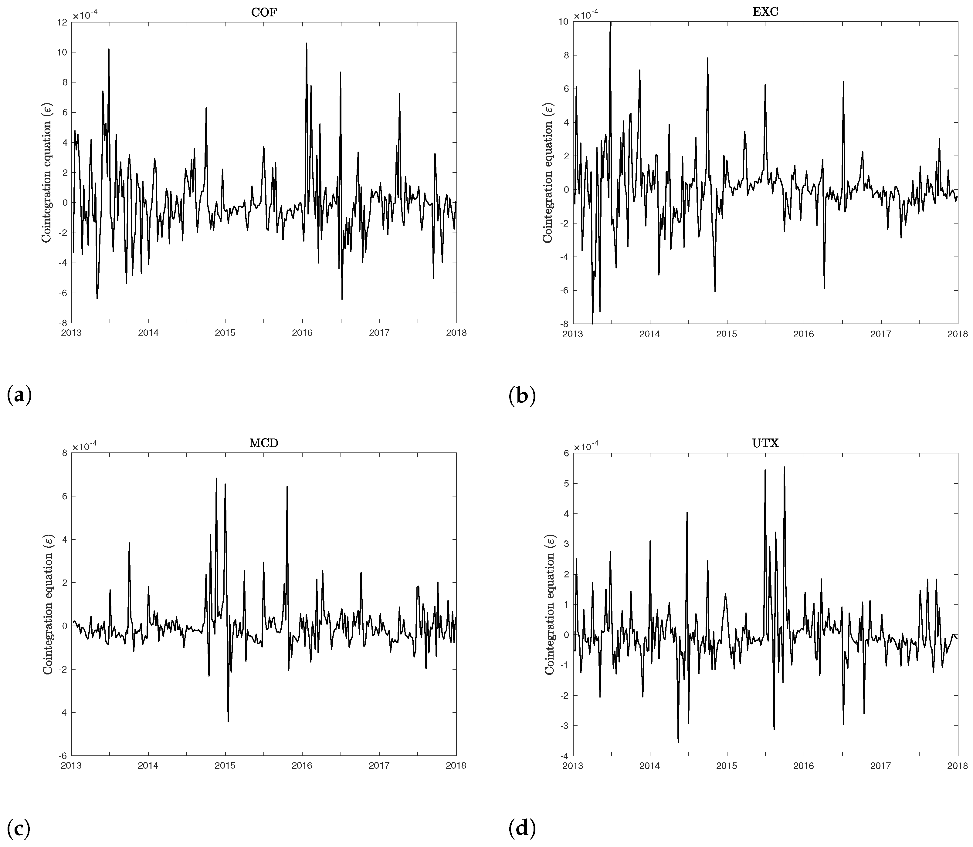
These are the variables that structural models of default predict as determinants of default probabilities and, therefore, credit spreads. If the variables are random walks and cointegrated, then the error term ${\epsilon }_{i,t}$ is stationary for all i. Figure 3 plots the residuals of the regressions (11) for the same four companies taken into consideration in Figure 2. Visual inspection, supported by unit root tests, confirms the presence of cointegration between the CDS spreads, leverage, and volatility. The same conclusions regarding the existence of a cointegrating vector apply to the whole sample of firms, as well as to CDS spreads for different maturities.

The autoregressive distributive lag, ARDL$(1,1,1)$, dynamic panel specification of (11) (with exogenous variables, $\Delta \mathbf{X}$) is defined as

$$\begin{array}{cc}\hfill {\mathrm{CDS}}_{i,t}& ={\alpha }_i+{\varphi }_i{\mathrm{CDS}}_{i,t-1}+{\beta }_{i,0}{\mathrm{LEV}}_{i,t}+{\beta }_{i,1}{\mathrm{LEV}}_{i,t-1}+{\gamma }_{i,0}{\mathrm{VOL}}_{i,t}+{\gamma }_{i,1}{\mathrm{VOL}}_{i,t-1}\hfill \\ \hfill & +{\mathit{\xi }}^{\top }\Delta {\mathbf{X}}_t+{\eta }_{i,t},\hfill \end{array}$$

(12)

and the error correction reparameterization of (12) is

$$\begin{array}{cc}\hfill \Delta {\mathrm{CDS}}_{i,t}& ={\lambda }_i\left({\mathrm{CDS}}_{i,t-1}-{\theta }_{i,0}-{\theta }_{i,L}{\mathrm{LEV}}_{i,t-1}-{\theta }_{i,V}{\mathrm{VOL}}_{i,t-1}\right)+{\beta }_{i,0}\Delta {\mathrm{LEV}}_{i,t}+{\gamma }_{i,0}\Delta {\mathrm{VOL}}_{i,t}\hfill \\ & +{\mathit{\xi }}^{\top }\Delta {\mathbf{X}}_t+{\eta }_{i,t}\hfill \\ \hfill & ={\lambda }_i{\epsilon }_{i,t-1}+{\beta }_{i,0}\Delta {\mathrm{LEV}}_{i,t}+{\gamma }_{i,0}\Delta {\mathrm{VOL}}_{i,t}+{\mathit{\xi }}^{\top }\Delta {\mathbf{X}}_t+{\eta }_{i,t}\hfill \end{array}$$

(13)

where ${\lambda }_i=-(1-{\varphi }_i)$, ${\theta }_{i,0}=\frac{{\alpha }_i}{1-{\varphi }_i}$, ${\theta }_{i,L}=\frac{{\beta }_{i,0}+{\beta }_{i,1}}{1-{\varphi }_i}$, and ${\theta }_{i,V}=\frac{{\gamma }_{i,0}+{\gamma }_{i,1}}{1-{\varphi }_i}$. The parameter ${\lambda }_i$ is the error-correcting speed of adjustment term. If ${\lambda }_i=0$, then there would be no evidence for a long-run relationship. This parameter is expected to be significantly negative under the prior assumption that the variables show a return to a long-run equilibrium. Of particular importance is the vector $\mathit{\theta }=\left({\theta }_L,{\theta }_V\right)$, which contains the long-run relationships between the variables driving the spreads.

Following [6], exogenous variables, in changes ($\Delta \mathbf{X}$), are also added. These are the change in level, slope and curvature of the term structure of interest rates, the log-return on the S&P500, and the change in the CBOE SKEW Index.

The level of interest rates is defined as the treasury yield for 5-year maturity. The slope of the term structure is defined as the difference between between 5-year and 1-year treasury yields. Although the spot rate is the only interest-rate-sensitive factor that appears in the firm value process, the spot rate process itself may depend upon other factors as well. For example, ref. [30] finds that the two most important factors driving the term structure of interest rates are the level and slope of the term structure. To capture potential nonlinear effects due to convexity, the squared level of the 5-year spot rate is also added as proxy for the curvature.

Similarly, the return on the S&P500 is used to proxy for the state of the economy. In fact, even if the probability of default remains constant for a firm, changes in credit spreads can occur due to changes in the expected recovery rate. The expected recovery rate in turn should be a function of the overall business climate.

Lastly, adding the changes in the CBOE SKEW Index aims at capturing the changes in the probability and magnitude of a large negative systematic jump, which ultimately would affect the firm value. Recent research ([4,9,31]) has in fact shown the crucial importance of allowing for jumps in the firm value process in order to explain short-term credit spreads. The CBOE SKEW Index is a strike-independent measure of the slope of the implied volatility curve that increases, as this curve tends to steepen. The index is calculated from the price of a tradable portfolio of out-of-the money S&P 500 options, similar to the VIX Index.

The choice of the variables (both endogenous and exogenous) mirrors the ones in [6]. However, three major differences need to be highlighted. First, here an ECM is estimated thus adding an additional stationary variable (the long-run equilibrium equation) to the regression in the spread changes. Secondly, the proposed calibration allows to estimate a firm-specific volatility (of both assets and equity), whilst they need to rely on a market-wide measure of volatility, namely the changes in the VIX index. Finally, the proxy for the downward jump risk employed here is different, as they calculate their own measure of skew based on the implied volatilities of options on the S&P 5000 futures. Here, the CBOE SKEW Index is used instead.

The estimation of the coefficients in (13) is carried through using the PMG estimator proposed by [32], which allows for heterogeneous short-run dynamics and common long-run equilibrium.

Table 6. ECM for 1-year CDS spreads. All the variables which structural models predict to influence the change in spreads are statistically significant and have the predicted signs. The loading on the cointegrating equation ($\epsilon$) is negative and statistically significant, thus confirming the existence of a long-term equilibrium to which spreads, volatility and leverage converge. This model constrains the long-run coefficient vector to be equal across panels while allowing for group-specific short-run and adjustment coefficients. The averaged short-run parameter estimates are reported.

1-Year CDS Spread
Long-Run Equilibrium
	Coefficient	t-Stat	p-Value
VOL	$\phantom{-}0.0028$	$\phantom{-}9.88$	$0.000$	***
LEV	$\phantom{-}0.0024$	$\phantom{-}14.45$	$0.000$	***
Short-term adjustment
	Coefficient	$\mathit{t}$-Stat	$\mathit{p}$-Value
$\epsilon$	$-0.1005$	$-11.52$	0.000	***
$\Delta$VOL	$\phantom{-}0.0074$	$\phantom{-}6.29$	$0.000$	***
$\Delta$LEV	$\phantom{-}0.0036$	$\phantom{-}5.23$	$0.000$	***
$\Delta$Level	$-0.0566$	$-4.55$	$0.000$	***
$\Delta$Slope	$\phantom{-}0.0213$	$\phantom{-}4.56$	$0.000$	***
$\Delta$Curvature	$\phantom{-}1.2409$	$\phantom{-}3.77$	$0.000$	***
$\Delta ln$(S&P500)	$-0.0013$	$-5.13$	$0.000$	***
$\Delta$Skew	$\phantom{-}5\times {10}^{-7}$	$\phantom{-}2.37$	$0.018$	**
Constant	$-0.0001$	$-9.66$	$0.000$	***

Number of observations: 16,640; number of groups: 64; observations per group: 260. Significance levels: 5% (**), 1% (***).

,

Table 7. ECM for 5-year CDS spreads. All the variables which structural models predict to influence the change in spreads are statistically significant and have the predicted signs. The loading on the cointegrating equation ($\epsilon$) is negative and statistically significant, thus confirming the existence of a long-term equilibrium to which spreads, volatility and leverage converge. This model constrains the long-run coefficient vector to be equal across panels while allowing for group-specific short-run and adjustment coefficients. The averaged short-run parameter estimates are reported.

5-Year CDS Spread
Long-Run Equilibrium
	Coefficient	t-Stat	p-Value
VOL	$\phantom{-}0.0225$	$\phantom{-}17.13$	$0.000$	***
LEV	$\phantom{-}0.0159$	$\phantom{-}15.54$	$0.000$	***
Short-term adjustment
	Coefficient	$\mathit{t}$-Stat	$\mathit{p}$-Value
$\epsilon$	$-0.0293$	$-9.60$	$0.000$	***
$\Delta$VOL	$\phantom{-}0.0252$	$\phantom{-}10.39$	$0.000$	***
$\Delta$LEV	$\phantom{-}0.0114$	$\phantom{-}7.69$	$0.000$	***
$\Delta$Level	$-0.0975$	$-4.90$	$0.000$	***
$\Delta$Slope	$\phantom{-}0.0346$	$\phantom{-}3.42$	$0.001$	***
$\Delta$Curvature	$\phantom{-}1.8381$	$\phantom{-}3.69$	$0.000$	***
$\Delta ln$(S&P500)	$-0.0025$	$-5.71$	$0.000$	***
$\Delta$Skew	$-6\times {10}^{-7}$	$-1.84$	$0.065$	*
Constant	$-0.0003$	$-9.75$	$0.000$	***

Number of observations: 16,640; number of groups: 64; observations per group: 260. Significance levels: 10% (*), 1% (***).

and

Table 8. ECM for 10-year CDS spreads. All the variables which structural models predict to influence the change in spreads are statistically significant and have the predicted signs. The loading on the cointegrating equation ($\epsilon$) is negative and statistically significant, thus confirming the existence of a long-term equilibrium to which spreads, volatility and leverage converge. This model constrains the long-run coefficient vector to be equal across panels while allowing for group-specific short-run and adjustment coefficients. The averaged short-run parameter estimates are reported.

10-Year CDS Spread
Long-Run Equilibrium
	Coefficient	t-Stat	p-Value
VOL	$\phantom{-}0.0335$	$\phantom{-}49.94$	$0.000$	***
LEV	$\phantom{-}0.0335$	$\phantom{-}28.24$	$0.000$	***
Short-term adjustment
	Coefficient	$\mathit{t}$-Stat	$\mathit{p}$-Value
$\epsilon$	$-0.0275$	$-5.18$	$0.000$	***
$\Delta$VOL	$\phantom{-}0.0399$	$\phantom{-}15.01$	$0.000$	***
$\Delta$LEV	$\phantom{-}0.0168$	$\phantom{-}7.86$	$0.000$	***
$\Delta$Level	$-0.1129$	$-4.95$	$0.000$	***
$\Delta$Slope	$\phantom{-}0.0242$	$\phantom{-}2.31$	$0.021$	**
$\Delta$Curvature	$\phantom{-}2.2031$	$\phantom{-}3.98$	$0.000$	***
$\Delta ln$(S&P500)	$-0.0027$	$-5.41$	$0.000$	***
$\Delta$Skew	$-9\times {10}^{-7}$	$-2.86$	$0.004$	***
Constant	$-0.0004$	$-5.31$	$0.000$	***

Number of observations: 16,640; number of groups: 64; observations per group: 260. Significance levels: 5% (**), 1% (***).

report the estimates of the long-run equilibrium equation in (11) and the short-term adjustment in (13). All the coefficients have the predicted sign and are highly statistically significant.

Most of the results are qualitatively identical when 1-, 5- and 10-year spreads are used. For what concerns the long-run equilibrium, both volatility and leverage display a positive and statistically significant loading: an increase in either VOL or LEV lead to a larger level of the spread in the long run. Focusing on the short-term adjustment, changes in both the firm’s equity volatility and its financial leverage increase the change in the spread. In terms of economic significance, an increase of 1% in the firm’s volatility increases the CDS spread of 0.7, 2.5 and 4 bps for 1-, 5- and 10-year maturity, respectively. Similarly, an identical change in the firm’s financial leverage induces the spread to undergo increases of 0.4, 1.1 and 1.7 bps, ceteris paribus. Thus, when considering the short-term adjustment, changes in the variable driving the long-equilibrium have an impact on the spreads, which increase with the maturity of the CDS contract.

For what concerns the set of exogenous variables, all the variables display significant coefficients. First, the changes in the level of interest rates have a negative impact on the credit spread: as pointed out by [33], the static effect of a higher spot rate is to increase the risk-neutral drift of the firm value process. A higher drift reduces the probability of default, and in turn, reduces the credit spreads. Ref. [34] obtains similar results. Likewise, the positive coefficients of the changes on the slope and curvature of the term structure are consistent with the findings of previous studies. As a decrease in yield curve slope may imply a weakening economy, it is reasonable to believe that the expected recovery rate might decrease in times of recession. Therefore, this would further decrease the credit spreads. Additionally, positive returns in the S&P500—which accounts for the growing economy and therefore an increasing expected recovery rate—have the effect of reducing the spread as suggested by economic intuition.

Finally, the coefficient reflecting the effect of systematic downward jumps (proxied as changes in the CBOE SKEW Index) is the only estimate whose sign differs between short- versus medium- and long-term spreads. As shown in [4,9,31], jumps are necessary to explain the level of short-term spreads: structural models which account only for diffusive shocks in the asset value process imply zero instantaneous probability of default and therefore cannot meet the observed levels of 6-month and 1-year spreads. Hence, the coefficient of $\Delta$Skew is positive for 1-year spread changes as expected.

An increase in the probability of a negative systematic jump translates into larger shot-term spreads. However, for longer maturities, the coefficient is negative. This apparently counterintuitive result can be easily explained by how systematic negative jumps affect firms. If such an event occurs, the ability of firms to repay its debt affects those liabilities expiring in the immediate future. This is what is observed for spreads with 1-year maturity. Conversely, if the firms survive the shot-term shock, they are more likely to be able to survive the futures shocks. Thus, the medium- and long-term spreads lower. Additionally, it is worth highlighting that, in the case of 5-year spreads, the impact of negative jumps is only marginally significant.

To conclude, a further analysis of the cointegration mechanism between spreads, volatility and financial leverage is discussed. As expected, the estimated coefficient of the long-run equation ($\epsilon$) is negative, within the unit circle and statistically significant. The closer the estimate is to zero, the slower the adjustment. Conversely, the closer to $-1$, the faster the adjustment. If $\lambda =-1$, there is full correction in 1 period, and if $\lambda <-1$ there is overshooting, that is an oscillatory adjustment dynamic. If $\lambda >0$, there is not cointegration, that is the disequilibrium expands. As expected, the size of the coefficient is larger, in absolute value, for shorter maturities: short-term spreads adjust faster to shocks in the firm’s volatility and leverage. The associated t-statistic is also larger for 1-year spread changes. Conversely, the degree of cointegration becomes stronger at longer horizons: the t-statistics of the long-run equilibrium equation increase with the maturity of the CDS.

To quantify the speed of convergence towards the long-run equilibrium, half-life statistics can be considered. The estimated negative loading of the cointegrating equation, $\widehat{\lambda }$, in (13) signifies that $-100·\widehat{\lambda }\%$ of that disequilibrium is dissipated before the next time period and $-100·(1-\widehat{\lambda })\%$ remains. It is often of interest to estimate how long it will take for an existing disequilibrium to be reduced by 50% (half-life of disequilibrium), that is

$$\text{half-life}=\frac{ln\left(0.5\right)}{ln(\widehat{\lambda }-1)}.$$

The estimated half-lives are 6.5, 23.3 and 24.9 weeks for the 1-, 5- and 10-year CDS spread, respectively. This highlights a significantly different behavior of the short- versus the medium- and long-term spreads: the short 1-year spreads reacts about four time faster than the 5- and 10-year spreads in order to realign to equilibrium. This finding is not surprising, as, given the shorter maturity, the spread should be expected to vary as quickly as possible with the changes in the firm’s leverage and volatility.

5. Discussion on the Main Results and Robustness Checks

In this section, we first examine how the compound option performs in terms of pricing errors (compared to other structural models); then, we compare our results on the cointegration analysis with those reported in other studies which document the inability of the proposed variables to explain the level and changes in credit spreads.

In order to compare the ability of the compound option model to price credit spreads, the results reported by [3] are used. There, the authors calibrate seven different structural models of default with different desirable features. More specifically, they analyze the performance of the following models: a baseline simple model with and without stochastic interest rates ([33]), a model with endogenous default barrier ([23]), a model with strategic default ([35,36]), a model with mean-reverting leverage ratios ([37]), a model with countercyclical market risk premium, and a jump-diffusion model. All the models underpredict credit spreads. Average absolute mean errors are reported in

Table 9. Average absolute mean errors (expressed in basis points) based on the results in [3]. There, the authors analyze the ability of structural models of default to reproduce observed credit spreads. They test a simple baseline model with and without stochastic interest rates ([33]), a model with endogenous default barrier ([23]), a model with strategic default ([35,36]), a model with mean-reverting leverage ratios ([37]), a model with countercyclical market risk premium, and a jump-diffusion model. A loss given default parameter of 48.69% is used by the authors for their calibration.

Structural Model	AAME
Baseline ([33])	$89.49$
Baseline plus stochastic interest rates ([33])	$105.67$
Endogenous default barrier ([23])	$86.27$
Strategic default ([35,36])	$76.89$
Mean-reverting leverage ratios ([37])	$93.25$
Countercyclical market risk premium ([3])	$83.19$
Jump-diffusion ([3])	$84.78$
Compound option model	$9.58$

. Similarly, the compound option model ($w=1/3$ and LGD = $50\%$) generally underpredicts the spread. However, the extent of the underpricing is much smaller: the proposed model is able to reduce the underpricing to 9.58 bps, whist the pricing errors of other structural models range from 83.19 to 105.67 bps.

Given the extent of the reduction in the pricing error, it is worth stressing further how the model implied spreads are calculated. In terms of market variables, the model spread depends (via the risk-neutral probabilities) on the equity value, the leverage of the company, the level of interest rates and the asset volatility. The proposed methodology is able to estimate the asset volatility and value at time t, using the known capital structure as well as the stock price. Once this volatility is estimated, say ${\sigma }_{V,t}^{\star }$, it is then used one week ahead to predict the spread. Therefore the spread at time $t+1$ is essentially a function such as ${\widehat{\mathrm{CDS}}}_{t+1}=f(S_{t+1},r_{r+1},{\mathrm{LEV}}_{t+1},{\sigma }_{V,t}^{\star })$, where the listed variables are the contemporaneous stock price, level of interest rates, leverage and the previous-week asset volatility, respectively. As r and LEV are unlikely to vary substantially from week to week, the proposed estimation shows how the equity, alongside the past volatility, is a sufficient statistic for predicting spreads in a compound option model.

However, it may be argued that what is being shown is simply predicting the credit spread at time $t+1$ with the credit spread at time t. This issue might be very impactful on the analysis, as the CDS data do show a significant autoregressive component (which is indeed modeled in the next section). In order to address this concern, the following variables are calculated:

$$X_t={\mathrm{CDS}}_t-{\mathrm{CDS}}_{t-1},Y_t={\mathrm{CDS}}_t-{\widehat{\mathrm{CDS}}}_t,$$

where CDS is the observed market spread, and $\widehat{\mathrm{CDS}}$ is the spread estimated with the proposed methodology. Given the results discussed in the previous sections, the test is conducted setting LGD = 50% and $w=1/3$. If this analysis is actually using the past spread to predict the current one, the distributions of X and Y should be, if not identical, relatively similar.

Thus, the two-sample Kolmogorov–Smirnov test is conducted on X and Y for each company in the dataset. Under the null hypothesis, X and Y are drawn from the same distribution. For brevity, the results of the test are omitted but available upon request. In the case of 1- and 5-year spreads, the null hypothesis is always rejected; for the 10-year spread, there are only two companies for which the test fails to reject the null hypothesis at 5% significance level. Given these results, it can be fairly concluded that the proposed model and estimation technique do not price the contemporaneous spread as the spread realized in the previous period.

To conclude, the sensible reduction in terms of underpricing may suggest that the compound option mechanism is better able to capture the default dynamics. Unfortunately [3] do not analyze the compound option model in [5], as it is not analytically tractable for their calibration approach. Better fits are only obtained by [4]; however, their model with stochastic asset volatility and jumps is far more complicated to calibrate than the proposed compound option model of default.

Regardless of the better ability of the compound option model to produce credit spreads, the use of a cointegration mechanisms is also able to enhance the fit of the regressions on the spreads as compared with [6] and other studies. For each firm i, the adjusted-$R^2$s of the short-term adjustment is calculated and reported in

Table 10. Adjusted $R^2$s of the firm-specific time-series regressions in (13) (short-term adjustments). As shown by both the mean- and median-adjusted $R^2$, the explanatory power of the variables, which should affect credit spread changes as predicted by structural models, diminishes with the maturity of the spread.

	1-Year	5-Year	10-Year		1-Year	5-Year	10-Year
Ticker	adj–${\mathit{R}}^2$			Ticker	adj–${\mathit{R}}^2$
AAPL	0.81	0.42	0.01	LLY	0.71	0.44	0.40
ABT	0.86	0.36	0.24	LOW	0.76	0.74	0.07
ALL	0.56	0.22	0.22	MCD	0.32	0.22	0.05
AMGN	0.62	0.38	0.30	MDT	0.92	0.88	0.79
BA	0.58	0.51	0.16	MMM	0.81	0.82	0.57
BAC	0.49	0.26	0.21	MO	0.65	0.41	0.19
BMY	0.71	0.29	0.15	MON	0.87	0.57	0.54
C	0.45	0.27	0.23	MRK	0.81	0.77	0.35
CAT	0.52	0.13	0.08	MS	0.63	0.53	0.50
CL	0.85	0.74	0.20	MSFT	0.90	0.59	0.15
CMCSA	0.57	0.20	0.13	ORCL	0.84	0.60	0.68
COF	0.87	0.72	0.73	OXY	0.71	0.33	0.14
COP	0.34	0.10	0.07	PEP	0.91	0.61	0.36
COST	0.89	0.89	0.87	PFE	0.64	0.43	0.19
CSCO	0.74	0.66	0.62	PG	0.86	0.82	0.20
CVS	0.75	0.57	0.24	PM	0.86	0.74	0.33
CVX	0.80	0.08	0.05	RTN	0.53	0.16	0.04
DD	0.66	0.39	0.43	SLB	0.36	0.12	0.05
DIS	0.77	0.46	0.32	SO	0.39	0.70	0.11
EMR	0.52	0.65	0.36	SPG	0.29	0.10	0.08
EXC	0.94	0.69	0.40	T	0.63	0.18	0.17
F	0.55	0.36	0.31	TGT	0.80	0.70	0.41
FDX	0.71	0.54	0.45	TWX	0.61	0.25	0.19
GD	0.81	0.81	0.76	TXN	0.81	0.40	0.44
GE	0.89	0.91	0.90	UNH	0.67	0.28	0.06
HAL	0.22	0.09	0.10	UNP	0.54	0.18	0.06
HD	0.79	0.55	0.33	USB	0.69	0.28	0.38
IBM	0.59	0.29	0.24	UTX	0.76	0.40	0.17
INTC	0.88	0.07	0.05	VZ	0.62	0.32	0.24
JNJ	0.77	0.50	0.47	WFC	0.62	0.53	0.52
JPM	0.57	0.41	0.39	WMT	0.71	0.33	0.09
KO	0.73	0.80	0.57	XOM	0.83	0.35	0.20
	1-year	5-year	10-year
	adj–$R^2$
Mean	0.69	0.45	0.30
Median	0.71	0.41	0.24
Min	0.22	0.07	0.01
Max	0.94	0.91	0.90

. Average adjusted-$R^2$s of 69%, 45% and 30% are obtained for 1-, 5- and 10-year spread changes. These numbers are significantly larger that the 26% (shot-maturity) and 21% (long-maturity) obtained by [6]. The results in [7] are not directly comparable, as the authors opt for regressing credit spread levels instead of changes onto similar sets of variables (still in levels). As the goodness to fit of the ECM model is evidently superior to the ones of a simple regression on changes, this provides extra evidence of the importance of a long-run equilibrium dynamic, which must be taken into account to correctly identify how credit spreads change.

Even when the implied volatility is used, the triplet spread, leverage, volatility still shows a statistically significant cointegration. However, using the average implied volatility of put options has a significant impact in the short-term adjustment dynamics: changes in the implied volatility are significant (at 10% significance level) only for the 1-year spread. Considering that most of equity options available in the market have maturity less than one year, the loss of significance for the 5- and 10-year spread should not surprise: the changes in the (short-term) implied volatility do not explain the reversion to the long-run equilibrium of medium- and long-term spreads. Nonetheless, the cointegration among the variables is still present, even though the model-implied volatility is replaced by the option-implied volatility.

These results, alongside the good pricing errors obtained via a compound option model of default, support the importance and ability of structural models in modeling the default as well as in explaining the level and changes of credit spreads.

Robustness Checks

Despite the proposed cointegration displaying much larger adjusted $R^2$s than previous works, the goodness of this approach is further investigated via principal components analysis (PCA), in a similar fashion to [7]. However, it is worth highlighting that the PCA conducted herein is on the CDS spread changes, whilst [7] do so on the levels. Based on the same arguments on the non-stationary of credit spreads discussed in the previous section, PCA should always be implemented on independent and identically distributed data (the changes) and not on random walks (the levels). Additionally, they look at raw credit spreads, whilst PCA requires demeaned variables to be used.

PCA aims at studying the extent to which the selected set of variables in (13) captures systematic credit-spread variations. PCA is, in fact, an effective tool for analyzing the cross-sectional variation of the spread changes, thereby searching for common ‘factors’ (the components) which should affect credit spread changes regardless of firm-specific characteristics.

First, the first 10 principal components (PCs) from the demeaned credit spreads changes are extracted for both the 1-, 5-, and 10-year maturities. Figure 4 shows the scree plots for the first 10 components. The spread changes for different maturities have similar principal components and display the kink around the 3rd/4th component. Overall, the first component explains 25–35% of the total variance of the spread changes; the second component explains around 15%; the third component explains around 10%; and the fourth component explains less then 10%. That is, in total, the first four components explain only about 60% of the total variance of the CDS spread changes. The fact that the first four component explain relatively little of the total variance points toward the possibility that variables influencing spread changes are firm-specific (as leverage and firm’s volatility) rather than systematic. This, alongside the successful cointegrating analysis, further supports the validity of the structural model of default to explain credit spreads.

These promising results could be, however, driven by over-fitting: as the volatility is obtained using the compound option model so to match the other market variables, the cointegrating mechanism could have been induced by the estimation methodology. In order to address this potential issue, the volatility estimated from the spread and the stock price is replaced by the option-implied volatility. More specifically, for each date, the option implied volatility surface is obtained from the most liquid out-of-the-money put options (i.e. out-of-the-money put options with daily trading volume above the annual mean volume), and their average is used. Option data are obtained from the OptionMetrics. The rational for focusing on put options is due to the fact part of the option skew displayed by equity option is attributable to the leverage effect ([38]). Therefore, the information conveyed by the implied volatility in the put region may have some relevance for the pricing of credit risk ([39]). Results are reported in

Table 11. ECM for 1-year CDS spreads using the average implied volatility of put options instead of ${\sigma }_S$. Similar results are obtained; however, the implied volatility is significant only at the 10% significance level in the short-term adjustment equation. Additionally, $\Delta$LEV, $\Delta$Curvature and $\Delta$Skew have become insignificant, and $\Delta$Level is significant at the 10% significance level only.

1-Year CDS Spread
Long-Run Equilibrium
	Coefficient	t-Stat	p-Value
IV	$\phantom{-}0.0008$	$\phantom{-}3.77$	$0.000$	***
LEV	$\phantom{-}0.0025$	$\phantom{-}12.18$	$0.000$	***
Short-term adjustment
	Coefficient	$\mathit{t}$-Stat	$\mathit{p}$-Value
$\epsilon$	$-0.1063$	$-9.79$	0.000	***
$\Delta$IV	$\phantom{-}0.0002$	$\phantom{-}1.83$	$0.067$	*
$\Delta$LEV	$\phantom{-}0.0012$	$\phantom{-}1.42$	$0.156$
$\Delta$Level	$-0.0390$	$-1.90$	$0.057$	*
$\Delta$Slope	$\phantom{-}0.0318$	$\phantom{-}3.17$	$0.002$	***
$\Delta$Curvature	$\phantom{-}0.5474$	$\phantom{-}1.41$	$0.157$
$\Delta ln$(S&P500)	$-0.0020$	$-5.22$	$0.000$	***
$\Delta$Skew	$\phantom{-}4\times {10}^{-7}$	$\phantom{-}1.35$	$0.176$
Constant	$\phantom{-}0.0001$	$2.31$	$0.000$	***

Number of observations:16,640; number of groups: 64; observations per group: 260. Significance levels: 10% (*), 1% (***).

,

Table 12. ECM for 5-year CDS spreads using the average implied volatility of put options instead of ${\sigma }_S$. Similar results are obtained; however, the implied volatility is not significant in the short-term adjustment equation. Additionally, $\Delta$LEV, $\Delta$Curvature and $\Delta$Skew are significant at the 10% significance level only, and $\Delta$Level is significant at the 5% significance level only.

5-Year CDS Spread
Long-Run Equilibrium
	Coefficient	t-Stat	p-Value
IV	$\phantom{-}0.0147$	$\phantom{-}8.67$	$0.000$	***
LEV	$\phantom{-}0.0038$	$\phantom{-}7.18$	$0.000$	***
Short-term adjustment
	Coefficient	$\mathit{t}$-Stat	$\mathit{p}$-Value
$\epsilon$	$-0.0360$	$-10.68$	$0.000$	***
$\Delta$IV	$\phantom{-}0.0002$	$\phantom{-}0.91$	$0.361$
$\Delta$LEV	$\phantom{-}0.0027$	$\phantom{-}1.93$	$0.053$	*
$\Delta$Level	$-0.1099$	$-2.19$	$0.028$	**
$\Delta$Slope	$\phantom{-}0.0886$	$\phantom{-}2.71$	$0.007$	***
$\Delta$Curvature	$\phantom{-}1.1884$	$\phantom{-}1.74$	$0.081$	*
$\Delta ln$(S&P500)	$-0.0045$	$-5.87$	$0.000$	***
$\Delta$Skew	$-1^{-6}$	$-1.90$	$0.057$	*
Constant	$-6^{-6}$	$-0.49$	$0.623$

Number of observations: 16,640; number of groups: 64; observations per group: 260. Significance levels: 10% (*), 5% (**), 1% (***).

and

Table 13. ECM for 10-year CDS spreads using the average implied volatility of put options instead of ${\sigma }_S$. Similar results are obtained; however, neither the implied volatility nor leverage are significant in the short-term adjustment equation. Additionally, $\Delta$Level, $\Delta$Slope, $\Delta$Curvature and $\Delta$Skew are significant at the 5% significance level only.

10-Year CDS Spread
Long-Run Equilibrium
	Coefficient	t-Stat	p-Value
IV	$\phantom{-}0.0312$	$\phantom{-}11.43$	$0.000$	***
LEV	$\phantom{-}0.0285$	$\phantom{-}17.22$	$0.000$	***
Short-term adjustment
	Coefficient	$\mathit{t}$-Stat	$\mathit{p}$-Value
$\epsilon$	$-0.0277$	$-5.82$	$0.000$	***
$\Delta$IV	$-2\mathrm{E}-05$	$-0.09$	$0.931$
$\Delta$LEV	$\phantom{-}0.0017$	$\phantom{-}1.07$	$0.283$
$\Delta$Level	$-0.1190$	$-2.24$	$0.025$	**
$\Delta$Slope	$\phantom{-}0.0814$	$\phantom{-}2.14$	$0.032$	**
$\Delta$Curvature	$\phantom{-}1.6594$	$\phantom{-}2.06$	$0.039$	**
$\Delta ln$(S&P500)	$-0.0055$	$-5.78$	$0.000$	***
$\Delta$Skew	$-2\times {10}^{-6}$	$-2.31$	$0.021$	**
Constant	$-0.0001$	$-5.43$	$0.000$	***

Number of observations: 16,640; number of groups: 64; observations per group: 260. Significance levels: 5% (**), 1% (***).

.

Secondly, credit spread changes for each company are regressed on an increasing set of PCs. For each set of PCs, the average adjusted-$R^2$ (and its standard deviation) are reported in

Table 14. Regression of both changes in CDS spreads (left columns) and residuals of (13) (right columns) onto an increasing set of principal components. Large average adjusted $R^2$s in the first columns should would translate a significant impact of systematic factors on spread changes. This does not appear to be the case. The pattern of the average adjusted $R^2$s obtained from regressing the PCs onto the residual of the ECM points should detect if some systematic factor could have been missed by (13). Mixed evidence is found regarding the first PC in the case of 5- and 10-year spreads.

1-Year CDS Spread
	$\Delta$CDS		$\mathit{\eta }$
PCs	mean adj–${\mathbf{R}}^{\mathbf{2}}$	st. dev. adj–${\mathbf{R}}^{\mathbf{2}}$	mean adj–${\mathbf{R}}^{\mathbf{2}}$	st. dev. adj–${\mathbf{R}}^{\mathbf{2}}$
1	0.089	0.202	0.068	0.166
2	0.087	0.211	0.068	0.182
3	0.110	0.261	0.086	0.220
4	0.071	0.189	0.079	0.209
5	0.073	0.200	0.085	0.224
6	0.062	0.189	0.069	0.205
7	0.059	0.179	0.069	0.220
8	0.047	0.165	0.065	0.207
9	0.039	0.153	0.069	0.219
10	0.032	0.141	0.062	0.200
5-year CDS spread
	$\Delta$CDS		$\mathit{\eta }$
PCs	mean adj–${\mathbf{R}}^{\mathbf{2}}$	st. dev. adj–${\mathbf{R}}^{\mathbf{2}}$	mean adj–${\mathbf{R}}^{\mathbf{2}}$	st. dev. adj–${\mathbf{R}}^{\mathbf{2}}$
1	0.115	0.239	0.125	0.274
2	0.076	0.218	0.098	0.261
3	0.080	0.227	0.095	0.250
4	0.088	0.232	0.092	0.243
5	0.078	0.217	0.089	0.248
6	0.065	0.180	0.068	0.208
7	0.058	0.176	0.070	0.214
8	0.055	0.178	0.056	0.174
9	0.060	0.194	0.053	0.166
10	0.049	0.167	0.057	0.170
10-year CDS spread
	$\Delta$CDS		$\mathit{\eta }$
PCs	mean adj–${\mathbf{R}}^{\mathbf{2}}$	st. dev. adj–${\mathbf{R}}^{\mathbf{2}}$	mean adj–${\mathbf{R}}^{\mathbf{2}}$	st. dev. adj–${\mathbf{R}}^{\mathbf{2}}$
1	0.118	0.248	0.100	0.215
2	0.096	0.243	0.086	0.225
3	0.102	0.263	0.093	0.233
4	0.091	0.243	0.080	0.213
5	0.096	0.252	0.084	0.217
6	0.065	0.208	0.069	0.192
7	0.065	0.207	0.071	0.184
8	0.055	0.199	0.063	0.182
9	0.047	0.178	0.057	0.167
10	0.047	0.176	0.058	0.165

. Ref. [7] reports simple $R^2$ instead of its adjusted correction for the number of regressors. This is incorrect, as adding an extra regressor is likely to increase the $R^2$, but not the adjusted-$R^2$, even when the variable (here, the PC) is not statistically significant. Then, the same set of PCs is regressed onto the residuals of (13). If the variables used to explain credit spread changes are not capturing systematic variations, large incremental adjusted-$R^2$ should be found from the regression of the residuals.

In general, the average adjusted-$R^2$s of the regressions of PCs on both the spread changes and on the residual of the short-term adjustment (13) are around 10%, thus signaling a very modest impact of systematic factors in explaining the cross-sectional variation of spread changes. The presence of a systematic factor related to the first principal components appears to be slightly more important for the medium- and long-term spreads. This could relate to how jump risk affect CDS spread changes for longer maturities. Perhaps using the change in the CBOE SKEW as a proxy for large jumps in the firms’ asset value is appropriate only when considering short-term spreads. This conjecture is based on the fact the average adjusted $R^2$ of the regression of the first component onto the 5-year residuals is actually larger than the average adjusted $R^2$ of the regression on the changes. Somehow, the short-term adjustment regression induces systematic risk in the residuals: the main difference between regression (13) estimated on the 5- and 10-year spread changes is the impact of the jumps, whose estimated coefficients also display the opposite sign. Alternatively, there is a systematic factor which the model is ignoring. This could be a liquidity factor for the CDS market; however, it would account only for a very small fraction of the cross-sectional variation of the CDS spread changes of longer maturities.

As last robustness check, the error correction parametrization in (13) is re-estimated for different values of the loss given default (60% and 80%). For the sake of brevity, the estimates are not reported but are available upon request. All the conclusions obtained in the previous section remain valid.

6. Conclusions

This paper develops a new estimation technique for the unobservable firm’s asset value and volatility which relies only on the observable equity value, risk-neutral probability of default and the face value of the firm’s debt.

The estimated parameters are first used to test the ability of model to reprice CDS spreads, out of sample. The pricing errors produced by the compound option model of default are then compared with those generated by the structural models in [3]. The compound option model sensibly outperforms the other models, being able to reduce the pricing error by almost 90%.

Secondly, the estimated parameters are used to investigate the existence of cointegration between credit spreads and those variables which structural models of default predict as driving their level. Estimations confirm the presence of an error-correction mechanism which leads to a long-equilibrium between the level of the spreads, financial leverage and the volatility of the firm’s equity. Once the cointegration equation is accounted for, the goodness to fit of the regressions on the changes improves substantially compared to previous studies. Finally, principal component analysis is employed to study the cross-sectional variation of credit spread changes.

Moreover, this work is the first to document the cointegration between CDS spreads, financial leverage and the firm’s risk in a large panel of US firms. Once the cointegration equation is added to the regressions on credit spread changes, the selected variables do explain quite well their variation. Consistently with previous findings and the economic intuition, it is shown that short-term spreads react more quickly to shocks to the long-run equilibrium, and that jumps affect short- and long-term spreads differently. Additionally, most of the variation in the cross-section appears to be driven by firm-specific characteristics rather than systematic factors.

One of the clear limitation of this work is related to the assumptions of the compound option model. In particular, the reference firm is assumed to default only at known discrete times which coincide with the reimbursement dates of the bonds outstanding. Furthermore, the exact amount of debt due at these future dates must be known (or sensibly approximated). As explained in Section 3.4, the maturities of the firm’s debt, as well as the aggregation scheme of the firm’s liabilities, had to be calibrated. The proposed calibration, though based on the ability of the compound option model to price the spreads, is somehow arbitrary, even though other calibration schemes were tested, showing that the results are robust. Finally, it would be interesting to relax the model assumption on the static capital structure: in fact, the firm is not allowed to modify its leverage throughout its lifetime. In the interests of brevity, these extensions are best left for future research.

References

1. Merton, R.C. On the pricing of corporate debt: The risk structure of interest rates. J. Financ. 1974, 29, 449–470. [Google Scholar]
2. Jones, E.P.; Mason, S.P.; Rosenfeld, E. Contingent Claims Analysis of Corporate Capital Structures: An Empirical Investigation. J. Financ. 1983, 39, 611–625. [Google Scholar] [CrossRef]
3. Huang, J.Z.; Huang, M. How Much of the Corporate-Treasury Yield Spread Is Due to Credit Risk? Rev. Asset Pricing Stud. 2012, 2, 153–202. [Google Scholar] [CrossRef]
4. Du, D.; Elkamhi, R.; Ericsson, J. Time-Varying Asset Volatility and the CreditSpread Puzzle. J. Financ. 2019, 74, 1841–1885. [Google Scholar] [CrossRef]
5. Geske, R. The Valuation of Corporate Liabilities as Compound Options. J. Financ. Quant. Anal. 1977, 12, 541–552. [Google Scholar] [CrossRef]
6. Collin-Dufresne, P.; Goldstein, R.S.; Martin, J.S. The Determinants of Credit Spread Changes. J. Financ. 2001, 56, 2177–2207. [Google Scholar] [CrossRef]
7. Cremers, K.J.M.; Driessen, J.; Meanhout, P.; Weinbaum, D. Individual Stock-Option Prices and Credit Spreads. J. Bank. Financ. 2008, 32, 2706–2715. [Google Scholar] [CrossRef]
8. Ericsson, J.; Jacobs, K.; Ovied, R. The Determinants of Credit Default Swap Premia. J. Financ. Quant. Anal. 2009, 44, 109–132. [Google Scholar] [CrossRef]
9. Zhang, B.Y.; Zhou, H.; Zhu, H. Explaining Credit Default Swap Spreads with the Equity Volatility and Jump Risks ofIndividual Firms. Rev. Financ. Stud. 2009, 22, 5099–5131. [Google Scholar] [CrossRef]
10. Engle, R.F.; Granger, C.W.J. Co-Integration and Error Correction: Representation, Estimation, and Testing. Econometrica 1987, 55, 251–276. [Google Scholar] [CrossRef]
11. Blanco, R.; Brennan, S.; Marsh, I.W. An Empirical Analysis of the Dynamic Relation between Investment-Grade Bonds and Credit Default Swaps. J. Financ. 2005, 60, 2255–2281. [Google Scholar] [CrossRef]
12. Eom, Y.H.; Helwege, J.; Huang, J.Z. Structural Models of Corporate Bond Pricing: An Empirical Analysis. Rev. Financ. Stud. 2004, 17, 499–544. [Google Scholar] [CrossRef]
13. Driessen, J. Is Default Event Risk Priced in Corporate Bonds? Rev. Financ. Stud. 2005, 18, 165–195. [Google Scholar] [CrossRef]
14. Longstaff, F.A.; Mithal, S.; Neis, E. Corporate Yield Spreads: Default Risk or Liquidity? New Evidence from the Credit Default Swap Market. J. Financ. 2005, 60, 2213–2253. [Google Scholar] [CrossRef]
15. Elton, E.J.; Gruber, M.J.; Agrawal, D.; Mann, C. Explaining the Rate Spread on Corporate Bonds. J. Financ. 2001, 56, 247–277. [Google Scholar] [CrossRef]
16. Campbell, J.Y.; Taksler, G.B. Equity Volatility and Corporate Bond Yields. J. Financ. 2003, 58, 2321–2349. [Google Scholar] [CrossRef]
17. Chen, L.; Collin-Dufresne, P.; Goldstein, R.S. On the Relation between the Credit Spread Puzzle and the Equity Premium Puzzle. Rev. Financ. Stud. 2009, 22, 3367–3409. [Google Scholar] [CrossRef]
18. Campbell, J.Y.; Cochrane, J.H. By Force of Habit: A Consumption-Based Explanation of Aggregate Stock Market Behavior. J. Political Econ. 1999, 107, 205–251. [Google Scholar] [CrossRef]
19. Leland, H.E. Corporate Debt Value, Bond Covenants, and Optimal Capital Structure. J. Financ. 1994, 49, 1213–1252. [Google Scholar] [CrossRef]
20. Heston, S.L. A Closed-Form Solution for Options with Stochastic Volatility with Applications to Bond and Currency Options. Rev. Financ. Stud. 1993, 6, 327–343. [Google Scholar] [CrossRef]
21. Merton, R.C. On the pricing of contingent claims and the Modigliani-Miller theorem. J. Financ. Econ. 1977, 5, 241–249. [Google Scholar] [CrossRef]
22. Black, F.; Cox, J.C. Valuing corporate securities: Some effects of bond indenture provisions. J. Financ. 1976, 31, 351–367. [Google Scholar] [CrossRef]
23. Leland, H.E.; Toft, K.B. Optimal Capital Structure, Endogenous Bankruptcy, and the TermStructure of Credit Spreads. J. Financ. 1996, 51, 987–1019. [Google Scholar] [CrossRef]
24. Frey, R.; Sommer, D. The Generalization of the Geske-Formula for Compound Options to Stochastic InterestRates is Not Trivial—A Note. J. Appl. Probab. 1998, 35, 501–509. [Google Scholar] [CrossRef]
25. Geske, R. The Valuation of Compound Options. J. Financ. Econ. 1979, 7, 63–81. [Google Scholar] [CrossRef]
26. Geman, H.; Karoui, N.E.; Rochet, J.C. Change of numéraire, change of probability measure and option pricing. J. Appl. Probab. 1995, 32, 443–458. [Google Scholar] [CrossRef]
27. Brigo, D. Market Models for CDS Options and Callable Floaters. Risk Magazine, 2005. [Google Scholar]
28. Brigo, D.; Mercurio, F. Interest Rate Models: Theory and Practice; Springer Finance: Berlin/Heidelberg, Germany, 2006. [Google Scholar]
29. Duffie, D.; Singleton, K.J. Modeling Term Structures of Defaultable Bonds. Rev. Financ. Stud. 1999, 12, 687–720. [Google Scholar] [CrossRef]
30. Litterman, R.; Scheinkman, J. Common Factors Affecting Bond Returns. J. Fixed Income 1991, 1, 54–61. [Google Scholar] [CrossRef]
31. Zhou, C. The term structure of credit spreads with jump risk. J. Bank. Financ. 2001, 25, 2015–2040. [Google Scholar] [CrossRef]
32. Pesaran, M.H.; Shin, K.; Smith, R.P. Pooled mean group estimation of dynamic heterogeneous panels. Pool. Mean Group Estim. Dyn. Heterog. Panels 1999, 94, 621–634. [Google Scholar] [CrossRef]
33. Longstaff, F.A.; Schwartz, E. A simple approach to valuing risky fixed and floating rate debt. J. Financ. 1995, 50, 789–821. [Google Scholar] [CrossRef]
34. Duffee, G.R. The relation between treasury yields and corporate bond yield spreads. J. Financ. 1998, 53, 2225–2241. [Google Scholar] [CrossRef]
35. Anderson, R.W.; Sundaresan, S. Design and Valuation of Debt Contracts. Rev. Financ. Stud. 1996, 9, 37–68. [Google Scholar] [CrossRef]
36. Mella-Barral, P.; Perraudin, W. Strategic Debt Service. J. Financ. 1997, 52, 531–556. [Google Scholar] [CrossRef]
37. Collin-Dufresne, P.; Goldstein, R.S. Do Credit Spreads Reflect Stationary Leverage Ratios? J. Financ. 2001, 56, 1929–1957. [Google Scholar] [CrossRef]
38. Carr, P.; Wu, L. Leverage Effect, Volatility Feedback, and Self-Exciting Market Disruptions. J. Financ. Quant. Anal. 2017, 52, 2119–2156. [Google Scholar] [CrossRef]
39. Carr, P.; Wu, L. A Simple Robust Link Between American Puts and Credit Protection. Rev. Financ. Stud. 2011, 24, 473–505. [Google Scholar] [CrossRef]
40. Cox, J.C. The constant elasticity of variance option pricing model. J. Portf. Manag. 1996, 23, 15–17. [Google Scholar] [CrossRef]
41. Dupire, B. Pricing with a Smile. Risk 1994, 7, 18–20. [Google Scholar]
42. Henry-Labordère, P. Calibration of Local Stochastic Volatility Models to Market Smiles: A Monte-Carlo Approach. Risk Magazine, 23 October 2009; 16. [Google Scholar]
43. Black, F.; Scholes, M. The Pricing of Options and Corporate Liabilities. J. Political Econ. 1973, 81, 637–654. [Google Scholar] [CrossRef] [Green Version]
Figure 1. Continuation value (dashed and dotted line) and value (solid line) of the equity. Checking whether the continuation value of the equity S is greater than the face value of the bond F is equivalent to finding the value of the assets V greater than the default threshold V ¯ .
Computation 10 00155 g001
Figure 2. Time series of the 5-year CDS spreads (top), equity volatility (middle) and financial leverage (bottom) estimated as in (9) for four different companies: Capital One Financial (financials), Exelon (mining, energy and utilities), McDonald’s (retail, wholesale and services), and United Technologies (manufacturing). Visual inspection suggest non-stationarity and a strong comovement of the three variables. The non-stationarity of the time series is confirmed by unit root tests.
Computation 10 00155 g002
Figure 3. Cointegration equations (residuals of regression (11)) for four different companies: Capital One Financial (financials), Exelon (mining, energy and utilities), McDonald’s (retail, wholesale and services), and United Technologies (manufacturing). Visual inspection suggest stationarity, and therefore cointegration of CDS spreads, leverage, volatility and the treasury yield. Unit root tests confirm the stationarity of the residuals. (a) Financials; (b) mining, energy and utilities; (c) retail, wholesale and services; (d) manufacturing.
Computation 10 00155 g003
Figure 4. Scree plots for the first 10 PCs of the demeaned 1-, 5-, and 10-year CDS spread changes. The spread changes for different maturities have similar principal components and display the kink around the 3rd/4th component. Overall, the first component explains 25–35% of the total variance of the spread changes; the second component explains around 15%; the third component explains around 10%; the fourth component explains less then 10%. The first 10 PCs are able to explain 80% of the total variance for 1- and 10-year spread changes, and almost 90% of the total variance for the 5-year spread changes. However, the first four are able to explain only about 60% of the total variance.
Computation 10 00155 g004