Modeling of 2R Planar Dumbbell Stacker Robot Locomotion Using Force Control for Gripper Dexterous Manipulation

Abstract

This paper describes a novel approach to the robotic system’s dexterous manipulator arm design. A simulation model of the robotic system is developed in the MATLAB/Simulink environment. The designed gripper moves the dumbbells from one shelf to another using impedance and dynamics control. The novel approach to contact force control was tested. For the most accurate simulation, the size and mass parameters of the manipulator and dumbbells are determined. In addition, various force parameters such as normal, friction and damping were evaluated. The dynamic behavior of the robotic system was described by the Lagrange dynamics equations to find the acceleration of the robot’s joints during friction interaction, and the energy performance was described. The corresponding dynamic model and its analysis are the starting point for its successful solution. The analytical and numerical descriptions are obtained and can be further used for computer simulation of the system, calculation of dynamic constraints, optimization of manipulator design, synthesis of trajectory planner and motion control algorithms of dexterous manipulative robotic systems.

1. Introduction

The foundations of modern robotics are built on the concepts of kinematics and dynamics of articulated rigid bodies [1]. Practically, every robotics textbook starts with a description of robot configuration using joint angles and then uses them to introduce robot kinematics, dynamics and control [2]. A significant consequence of this is the implicit assumption of knowing its kinematic information: the arrangement of links and joints, the link dimensions and the joint positions to control a robot [3,4]. Assuming, in addition, that the link dimensions are constant, then the only information needed to control a robot is the joint angles [5]. Robot controllers still rely on the same principle—of general kinematics and measurable joint positions.

Since manipulation and force control continue to develop rapidly in modern robotics, only a few methods have been proposed to control robotic complexes [6,7,8]. Hence, this work describes the novel approach to the modeling and design of a 2R planar dexterous manipulation robot with a gripper that can grab dumbbells from a shelf and move it to another one. The novelty of the proposed approach lies in a completely unprecedented combination of uniquely designed gripping and dynamics/impedance force control methods for the stacking of dumbbells as a critical manipulation task.

The main objectives of the work are listed below:

• Mechanical Structure Analysis;
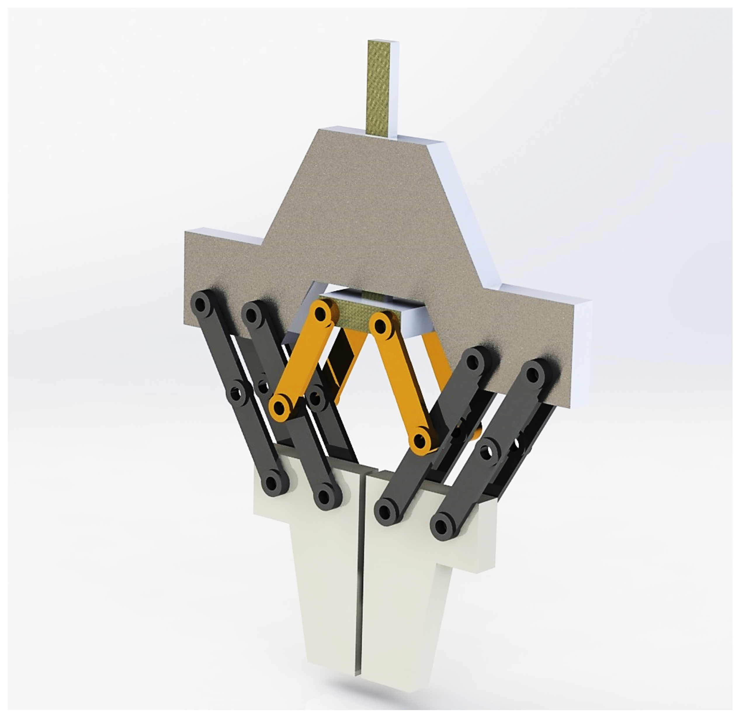
• Gripper Design;
• Kinematics;
• Dynamics;
• Model-based Control of Robot Dynamical Interaction with Environment;
• Contact Forces Set;
• Trajectory Set.

2. Materials and Methods

This work proposes the analysis of the dynamics methods:

• Euler–Newton formulation: to describe the bodies of the rigid dynamic, it is an effective way for complex systems and is used to assemble the equation of the motion using the algorithms;
• Lagrangian formulation: using the kinetic and potential energy of the robot, it is effective for simple systems with few bodies that have a degree of freedom.

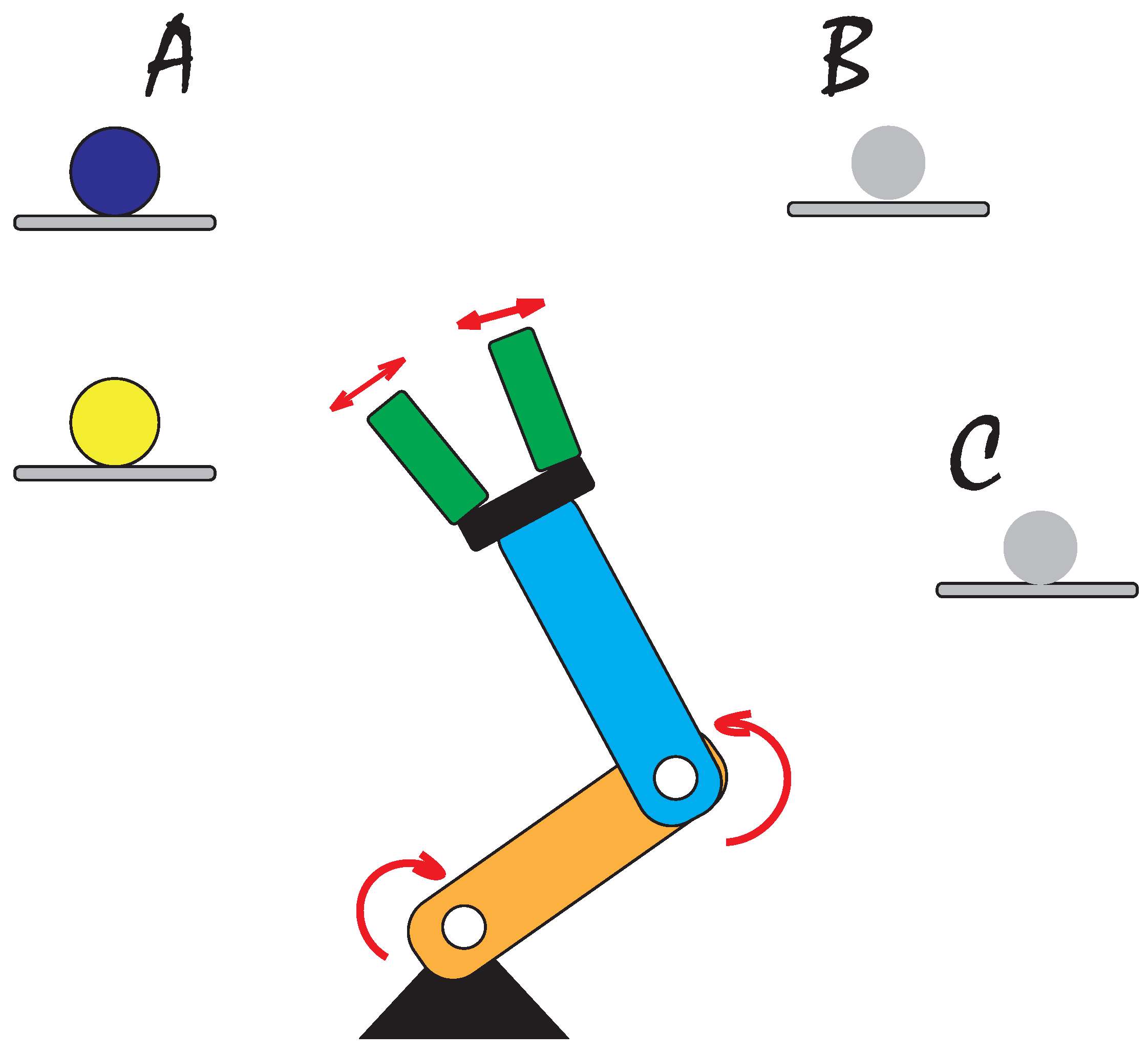
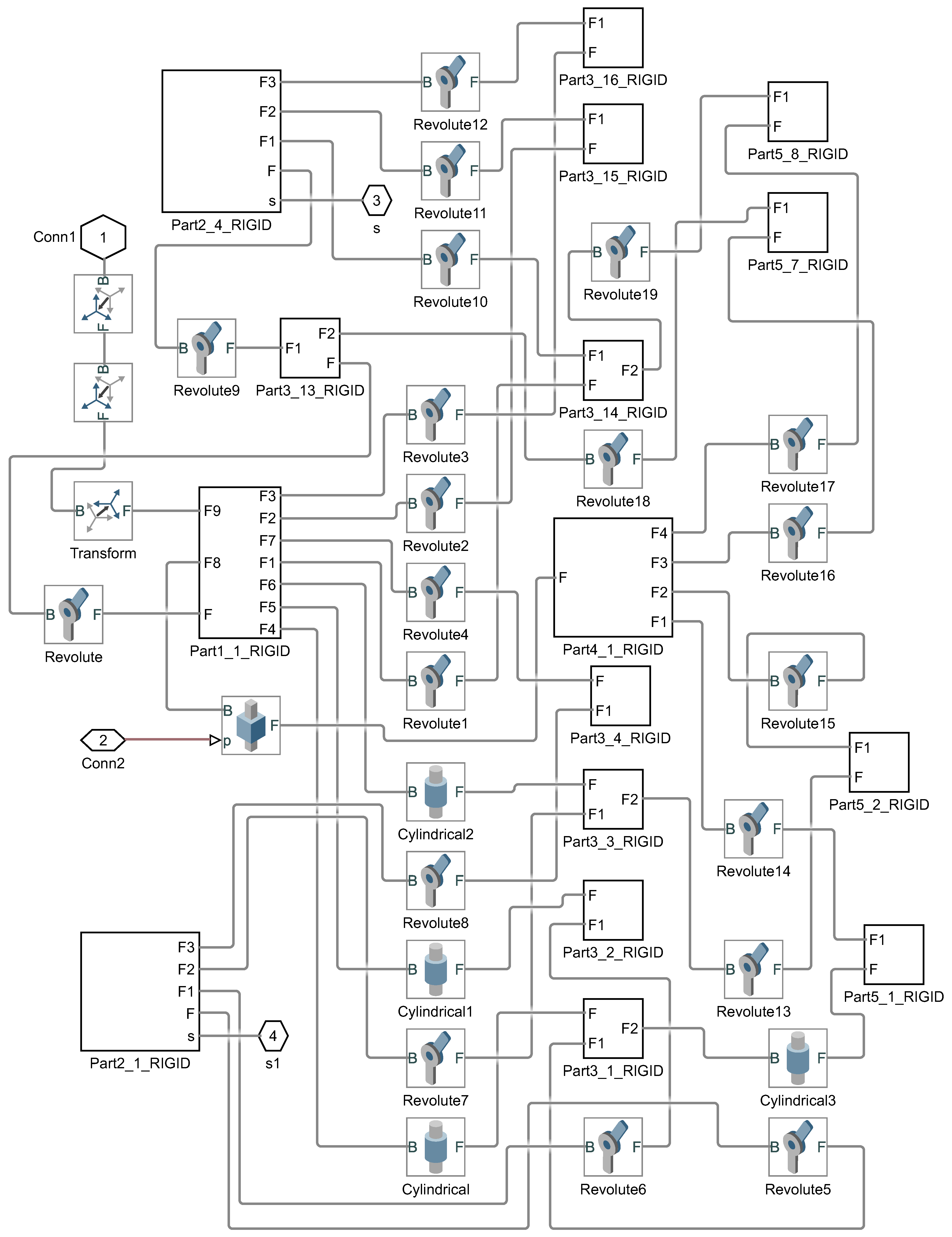
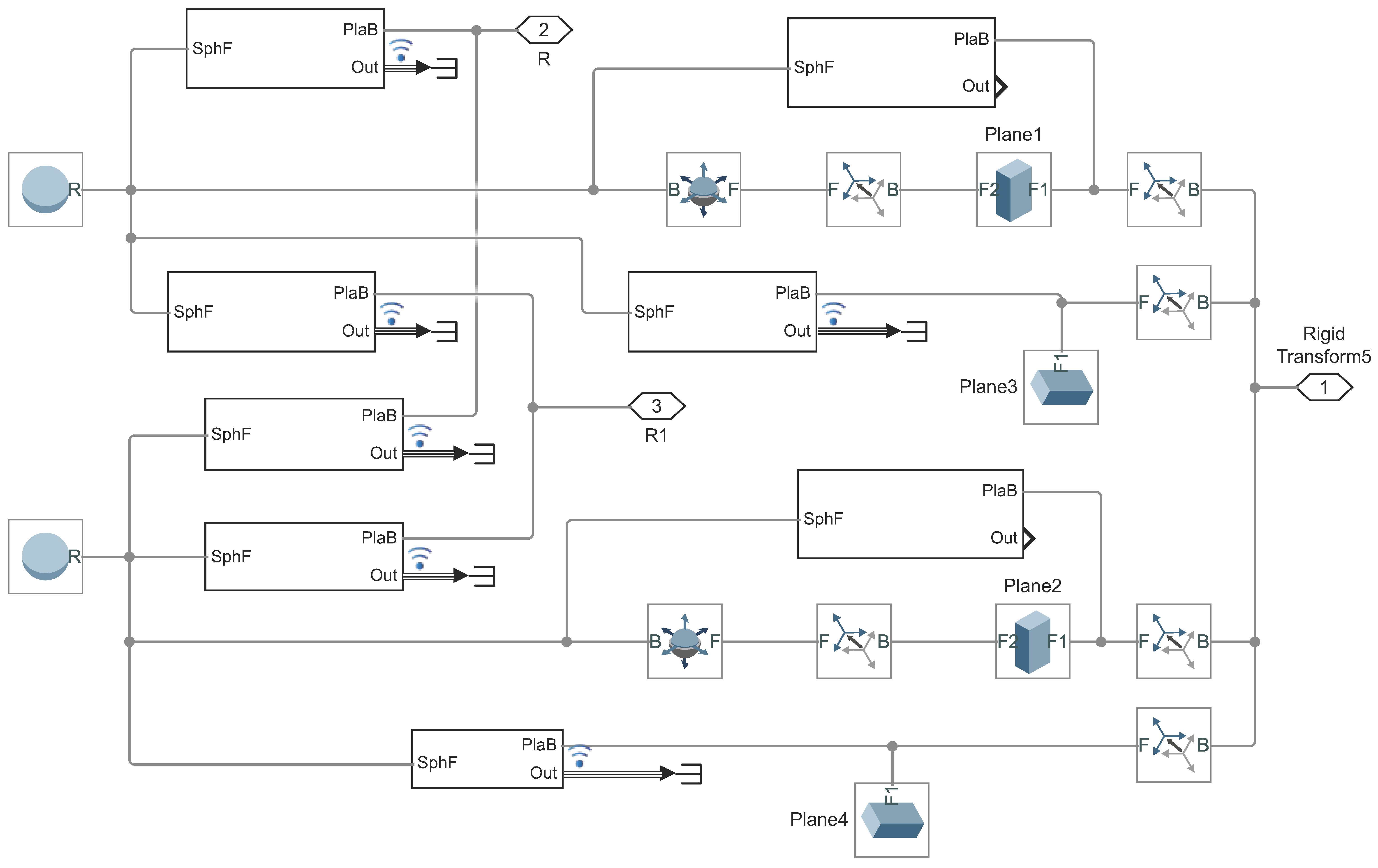
2.1. Mechanical Structure

The robot model comprises two revolute joints and two links that are shown on the robot scheme. The first and second links’ lengths are 0.8m each, and their masses are 2 kg, respectively. The links are connected with no elastic elements. The first link is connected to the ground, and the end effector is connected to the second link. The x-axis is to the right, the z-axis is in the upward direction, and the y-axis is out of the screen. The robot is equipped with a mechanical gripping device, which can be seen in Figure 1. The essence of the task is to move dumbbells from one shelf to another (from A to B or C, and back again), and the control of this system should be as accurate and energy efficient as possible for this type of manipulation.

The physical interface between a robot arm and the workpiece is called robot grippers. The most important part of the robot is the end-of-arm-tooling (EOAT). A robotic gripper is a device that enables the holding, handling, tightening and releasing of the object. A gripper is a component attached to a robot or a part of a fixed automated system. There are many styles and sizes of grippers that the application’s model can select.

Choosing a proper gripper is essential to ensure successful automation applications [9]. Robotic grippers are also called end effectors. The benefit of using grippers is reducing part damage to the product. The robotic grippers are manufactured and programmable with different functions, trading speed and flexibility force.

Robotic grippers with two fingers are the simplest grippers used in the industrial collaborative robots market. These are easy to manufacture. Different alternatives in the group, such as opening control, pressure control and distance control, are commonly used by collaborative robots companies with plug-and-play features in universal robots.

The proposed gripper (Figure 2) comprises 17 parts to constrain its motion. It is controlled by a prismatic joint in the MATLAB environment.

2.2. Forward Kinematics

The position of the end effector can be analyzed by its pose in relation to the base by describing the geometrical vectors, the position of the end effector is determined in Cartesian space, and the equations are considered as:

$$P_x=l_{1}cos{\theta }_1+l_{2}cos({\theta }_1+{\theta }_2);$$

(1)

$$P_y=l_{1}sin{\theta }_1+l_{2}sin({\theta }_1+{\theta }_2),$$

(2)

where $P_x$ and $P_y$ are the coordinates of the end effector position in x and y directions; $l_1$ and $l_2$ are the lengths of each link, and ${\theta }_1$ and ${\theta }_2$ are the angles of each joint, respectively.

Furthermore, the position matrix of the end effector can be described as shown:

$$P=\left[\begin{array}{c}{P}_x\\ P_y\end{array}\right]=\left[\begin{array}{c}{l}_{1}cos{\theta }_1+l_{2}cos({\theta }_1+{\theta }_2)\\ l_{1}sin{\theta }_1+l_{2}sin({\theta }_1+{\theta }_2)\end{array}\right].$$

(3)

The velocity matrix of the end effector is written as:

$$V=\left[\begin{array}{c}\dot{P_x}\\ \dot{P_y}\end{array}\right]=\left[\begin{array}{c}-l_1\dot{{\theta }_1}sin{\theta }_1-l_2(\dot{{\theta }_1}+\dot{{\theta }_2})sin({\theta }_1+{\theta }_2)\\ l_1\dot{{\theta }_1}cos{\theta }_1+l_2(\dot{{\theta }_1}+\dot{{\theta }_2})cos({\theta }_1+{\theta }_2)\end{array}\right].$$

(4)

The parameters of the space angular velocities are extracted as shown:

$$V=\left[\begin{array}{cc}-l_{1}sin{\theta }_1-l_{2}sin({\theta }_1+{\theta }_2)& -l_{2}sin({\theta }_1+{\theta }_2)\\ l_{1}cos{\theta }_1+l_{2}cos({\theta }_1+{\theta }_2)& l_{2}cos({\theta }_1+{\theta }_2)\end{array}\right]\left[\begin{array}{c}\dot{{\theta }_1}\\ \dot{{\theta }_2}\end{array}\right]=J(\theta )\dot{\theta },$$

(5)

where $J(\theta )$ is the Jacobian of the planar 2R robot and $\theta$ is the vector of angular velocities.

$$J(\theta )=\left[\begin{array}{cc}-l_{1}sin{\theta }_1-l_{2}sin({\theta }_1+{\theta }_2)& -l_{2}sin({\theta }_1+{\theta }_2)\\ l_{1}cos{\theta }_1+l_{2}cos({\theta }_1+{\theta }_2)& l_{2}cos({\theta }_1+{\theta }_2)\end{array}\right].$$

(6)

After identifying these kinematic parameters of the system, it is necessary to proceed to the dynamic behavior of the presented robotic system.

2.3. Robot Dynamics

Contact forces are transmitted between bodies by short-range atomic or molecular interactions [10]. For example, push, pull, the tension of a string, normal force, the force of friction, etc. The origin of these forces can be explained in terms of the fundamental properties of matter. However, this approach emphasizes the properties of these forces and the techniques for dealing with physical problems, not worrying about their microscopic origins. To implement the contact forces in this case, they have to be applied to the gripper’s fingers, the dumbbell and between the dumbbell and the shelf.

The forces and torques are considered, as the forward dynamics have to determine the robot’s acceleration $\ddot{\theta }$ for the joint space $(\theta ,\dot{\theta })$, the forces on the joints F and torques $\tau$. Furthermore, the inverse dynamics determine the robot’s forces F and torques $\tau$ for the robot acceleration $\ddot{\theta }$. The Lagrangian formulation is considered for analyzing this robot system.

The Lagrangian function is the difference between the kinetic energy K and potential Energy U, as shown:

$$L(\theta ,\dot{\theta })=K(\theta ,\dot{\theta })-U(\theta ,\dot{\theta }).$$

(7)

The total kinetic energy for both links is calculated.

$$K(\theta ,\dot{\theta })=K_1(\theta ,\dot{\theta })+K_2(\theta ,\dot{\theta })=\frac{m_1{v}_1^2}{2}+\frac{m_2{v}_2^2}{2},$$

(8)

where $v_1$ and $v_2$ are the linear velocity of the first and second links, respectively.

The total potential energy of both links is

$$U(\theta ,\dot{\theta })=U_1(\theta ,\dot{\theta })+U_2(\theta ,\dot{\theta })=m_{1}g{h}_1+m_{2}g{h}_2,$$

(9)

where $h_1$ and $h_2$ represent the heights of the center of masses for the first and second links.

To determine the velocities of the center of mass for both links:

$$V_1^2=\dot{P_1^2}=\dot{X_1^2}+\dot{Y_1^2}={\left(\frac{l_1}{2}\dot{{\theta }_1}sin{\theta }_1\right)}^2+{\left(\frac{l_1}{2}\dot{{\theta }_1}cos{\theta }_1\right)}^2=\frac{\dot{{\theta }_1^2}{l}_1^2}{2};$$

(10)

$$V_2^2=\dot{P_2^2}=\dot{X_2^2}+\dot{Y_2^2}=\left(l_1^2+l_1{l}_{2}cos{\theta }_2+\frac{l_2^2}{4}\right)\dot{{\theta }_1^2}+\left(l_1{l}_{2}cos{\theta }_2+\frac{l_2^2}{4}\right)\dot{{\theta }_1}\dot{{\theta }_2}+\frac{\dot{{\theta }_2}{l}_2^2}{4}.$$

(11)

The kinetic energy for both links:

$$K_1(\theta ,\dot{\theta })=\frac{m_1{v}_1^2}{2}=\frac{m_1\dot{{\theta }_1^2}{l}_1^2}{8};$$

(12)

$$K_2(\theta ,\dot{\theta })=\frac{m_2}{2}\left[\frac{m_2{v}_2^2}{2}=\left(l_1^2+l_1{l}_{2}cos{\theta }_2+\frac{l_2^2}{4}\right)\dot{{\theta }_1^2}+\left(l_1{l}_{2}cos{\theta }_2+\frac{l_2^2}{4}\right)\dot{{\theta }_1}\dot{{\theta }_2}+\frac{\dot{{\theta }_2}{l}_2^2}{4}\right].$$

(13)

The potential energy of the center of mass for both links can be presented as:

$$U_1(\theta ,\dot{\theta })=m_{1}g\frac{l_1}{2}sin{\theta }_1;$$

(14)

$$U_2(\theta ,\dot{\theta })=m_{2}g\left(l_{1}sin{\theta }_1+\frac{l_2}{2}sin({\theta }_1+{\theta }_2)\right);$$

(15)

The Lagrangian formulation is presented as shown:

$$\frac{d}{dt}\left(\frac{d\mathcal{L}}{d\dot{\theta }}\right)-\left(\frac{d\mathcal{L}}{d\theta }\right)={\tau }^T,$$

(16)

where $\tau$ is the applied torque for the joints $\tau =\left[{\tau }_1{\tau }_2\right]$, the equation of motion should be derived for both generalized coordinates.

For the first joint:

$$\frac{d{\mathcal{L}}_1}{d{\theta }_1}=-m_{1}g\frac{l_1}{2}cos{\theta }_1-m_{2}g{l}_{1}cos{\theta }_1-m_{2}g\frac{l_2}{2}-cos({\theta }_1+{\theta }_2);$$

(17)

$$\frac{d{\mathcal{L}}_1}{d\dot{{\theta }_1}}=\frac{1}{4}{m}_{1}g{l}_1^2\dot{{\theta }_1^2}+m_2\left(l_1^2+\frac{l_2^2}{4}\right)\dot{{\theta }_1^2}+(m_2{l}_1{l}_{2}cos{\theta }_2)\dot{{\theta }_1}+\left(\frac{1}{2}{m}_2{l}_1{l}_{2}cos{\theta }_2\dot{{\theta }_2}+\left(\frac{1}{4}{m}_2{l}_2^2\right)\right)\dot{{\theta }_2}.$$

(18)

For the second joint:

$$\frac{d{\mathcal{L}}_2}{d{\theta }_2}=-\left(\frac{1}{2}{m}_2{l}_1{l}_{2}sin{\theta }_2\right)\dot{{\theta }_1^2}-\left(\frac{1}{2}{m}_2{l}_1{l}_{2}sin{\theta }_2\right)\dot{{\theta }_1^2}\dot{{\theta }_2^2}-\left(\frac{1}{2}{m}_2{l}_{2}cos({\theta }_1+{\theta }_2)g\right);$$

(19)

$$\frac{d{\mathcal{L}}_2}{d\dot{{\theta }_2}}=\left(\frac{1}{2}{m}_2{l}_1{l}_{2}sin{\theta }_2\right)\dot{{\theta }_1^2}+\frac{1}{4}{m}_2{l}_2^2\dot{{\theta }_1}+\frac{1}{4}{m}_2{l}_2^2\dot{{\theta }_2}.$$

(20)

Now the applied torques on the joints can be obtained. The torque on the first joint:

$$\begin{array}{c}{\tau }_1=\left(\frac{1}{4}{m}_1{l}_1^2+m_2\left(l_1^2+l_1{l}_2\cos {\theta }_2+\frac{l_2^2}{4}\right)\right){\ddot{\theta }}_2+\frac{1}{4}{m}_2{l}_2\left(l_1\cos {\theta }_2+\frac{l_2}{2}\right)\ddot{{\theta }_2}-\frac{1}{2}{m}_2{l}_1{l}_2\sin {\theta }_2\left(2{\dot{\theta }}_1{\dot{\theta }}_2+{{\dot{\theta }}_2}^2\right)+\hfill \\ \hfill +\left(\frac{1}{2}{m}_1+m_2\right)g{l}_1\cos \left({\theta }_1+{\theta }_2\right).\end{array}$$

(21)

The torque on the second joint:

$${\tau }_2=\left(\frac{1}{2}{m}_2{l}_2\left(l_{1}cos{\theta }_2+\frac{l_2}{2}\right)\right){\ddot{\theta }}_1+\frac{1}{4}{m}_2{l}_2^2\ddot{{\theta }_2}+\frac{1}{2}{m}_2{l}_1{l}_{2}sin\left({\theta }_2\right){{\dot{\theta }}_1}^2+\frac{1}{2}{m}_{2}g{l}_2\cos \left({\theta }_1+{\theta }_2\right).$$

(22)

The torques of the joints can be described by the matrix equation of the motion:

$$M\left(\theta \right)\ddot{\theta }+C\left(\theta ,\dot{\theta }\right)\dot{\theta }+G\left(\theta \right)={\tau }_d^T,$$

(23)

where $\theta$, $\dot{\theta }$, $\ddot{\theta }$ are the position vector, angular velocity and angular acceleration of the joints; $M\left(\theta \right)$—the inertia matrix; $C\left(\theta ,\dot{\theta }\right)$—the Coriolis vector and centrifugal forces; $G\left(\theta \right)$—the vector of the potential energy; ${\tau }_d^T$—the inherent dynamics of the robot.

$$M\left(\theta \right)=\left[\begin{array}{cc}\frac{1}{4}{m}_1{l}_1^2+m_2\gamma & \frac{1}{2}{m}_2{l}_2\left(\epsilon +\frac{1}{2}{l}_2\right)\\ \frac{1}{2}{m}_2{l}_2\left(\epsilon +\frac{1}{2}{l}_2\right)& \frac{1}{2}{m}_2{l}_2^2\end{array}\right];$$

(24)

$$C\left(\theta ,\dot{\theta }\right)\dot{\theta }=\left[\begin{array}{c}-\frac{1}{2}{m}_2{l}_1{l}_{2}sin{\theta }_2\left(2{\dot{\theta }}_1{\dot{\theta }}_2+{{\dot{\theta }}_2}^2\right)\\ \frac{1}{2}{m}_2{l}_1{l}_{2}sin{(\theta }_2){{\dot{\theta }}_1}^2\end{array}\right];$$

(25)

$$G\left(\theta \right)=\left[\begin{array}{c}\left(\frac{1}{2}{m}_1+m_2\right)g{l}_{1}cos\left({\theta }_1+{\theta }_2\right)+\frac{1}{2}{m}_{2}g{l}_2\cos \left({\theta }_1+{\theta }_2\right)\\ \frac{1}{2}{m}_2{gl}_{2}cos\left({\theta }_1+{\theta }_2\right)\end{array}\right],$$

(26)

where $\epsilon =l_{1}cos{\theta }_2$, $\gamma =l_1^2+l_2\epsilon +\frac{1}{4}{l}_2^2$ and $g=9.80665 {\mathrm{m}/\mathrm{s}}^2$.

The calculated $\tau$ is for the equilibrium of the initial position, so its effect corresponds to the gravity. To achieve motion for these joints, additional torques and forces should be added.

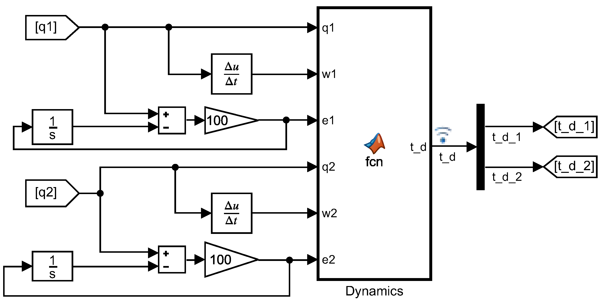
2.4. Robot Control

To achieve the motion of the desired trajectory of the robot, the total torques should include three components:

$${\tau }^T={\tau }_d^T+{\tau }_f^T+{\tau }_i^T,$$

(27)

here ${\tau }^T$ is the total applied torque on the joints required for the trajectory; ${\tau }_d^T$ is the inherent dynamics of the robot; ${\tau }_f^T$ is the friction torque and ${\tau }_i^T$ is the dynamic interaction with the environment. The friction torque can be determined:

$${\tau }_f^T=b\dot{\theta },$$

(28)

where b is the friction damping coefficient and $\dot{\theta }$ is the angular velocity of the generalized coordinates. The dynamic interaction with the environment is determined as

$${\tau }_i^T=J^T{F}^T,$$

(29)

where $J^T$ is the Jacobian matrix; $F^T$ is the externally applied force on the end effector.

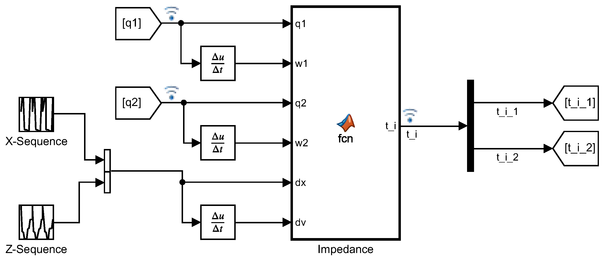
2.5. Impedance Control

When the interaction with the environment is considered, force F is the applied force on the end effector. To keep the robot in the equilibrium position, actuators have to produce reaction torque with equal power [11].

$$Fv=\tau \dot{\theta }=P,$$

(30)

where $F=\left[F_x{F}_y\right]$ is a vector of the external force; $v=\left[v_x{v}_y\right]$ is a velocity vector; $\tau =\left[{\tau }_1{\tau }_2\right]$ is a vector of torques on joints and P is a power in scalar.

The robot is treated as a virtual spring with elastic force F applied to the end effector to get the impedance behavior [12]

$$F^T=K\left(\tilde{P}-P\right)+D\left(\tilde{v}-v\right),$$

(31)

where K and D are proportional and derivative (or damping) coefficients, $\tilde{P}$ is the desired position and P is the current position, $\tilde{v}$ is the desired linear velocity of the end effector and v is the current velocity.

$$\tilde{P}=\left[\begin{array}{c}{A}_{x}cos\left(ft\right)+B_x\\ A_{y}cos\left(ft\right)+B_y\end{array}\right],$$

(32)

where $A_x$ and $A_y$ are the amplitudes and $B_x$ and $B_y$ are the biases for x and y, respectively, f is the frequency of oscillation and t is the time; the impedance control helps create a virtually passive system that can dynamically interact with the environment [13,14].

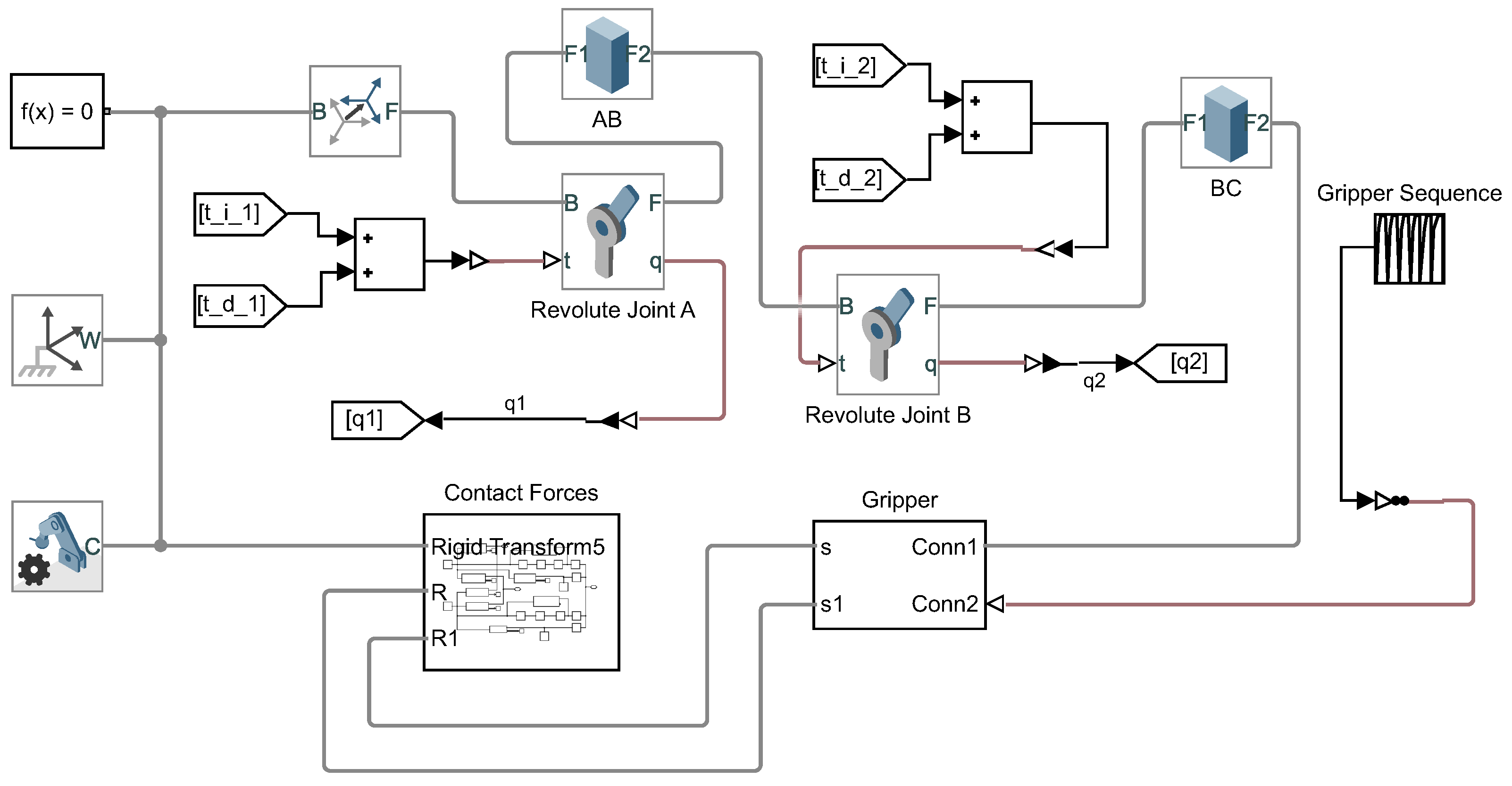
2.6. Simulink Model

A simulation model in the MATLAB/Simulink environment was developed. Simscape Multibody Library was primarily used in this research. Simulation modeling is a research method in which the understudy robotic system is replaced by a model that describes the actual system with sufficient accuracy. It is an efficient tool for conducting experiments to verify, evaluate and support design decisions, study the interaction between the components of the robot and the objects of the environment, as well as analyze kinematic and dynamic properties, adjust control algorithms and get other information about the system [15].

The robot model primarily comprises the main mechanical part (Figure 3), which includes control subsystems such as dynamic controller (Figure 4) and impedance controller (Figure 5). To connect the main parts of the robot with the working body, a subsystem of the gripper model is provided (Figure 6). A subsystem of contact forces (Figure 7) is provided to simulate the force interaction with the gripper and dumbbell surfaces.

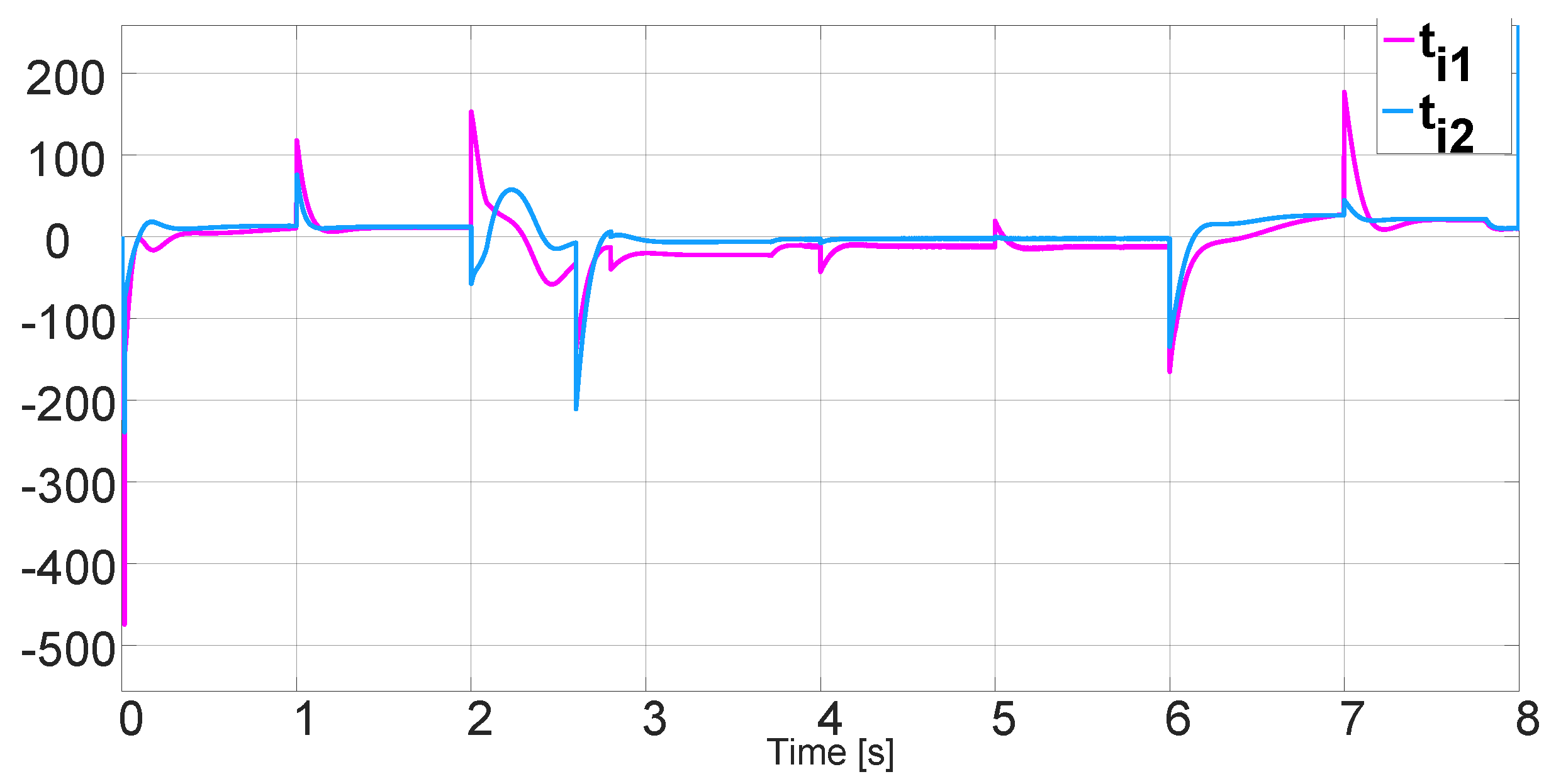
3. Results and Analysis

A simulation of the dexterous 2R manipulator model was carried out. The scene simulation time was set to 8 s. Plotted results of the modeling process are obtained.

Figure 8 and Figure 9 show the results of the impedance and dynamics outputs of the controllers. The change in the angles of each of the manipulator’s joints, strictly speaking, the configurations of each of the joints at each moment of time, is shown in Figure 10. Contact forces include three varieties: normal force, friction force and damping force. The change in these forces between the first and second finger gripper with the first dumbbell is shown in Figure 11 and Figure 12. The change in these forces between the first and second dumbbell fingers is shown in Figure 13 and Figure 14. The change in contact forces between the first and second dumbbell with the target shelf is shown in Figure 15 and Figure 16.

The image sequence of the simulated result of the robotic manipulator model from MATLAB Mechanics Explorer is shown in Figure 17 and Supplementary Materials.

The results show that the interaction forces of the individual first finger and the second finger of the gripper, specifically the friction force, are opposite in value, while the damping and normal force differ only imperceptibly. In summary, simulation errors are negligible when compared to results due to the effectiveness of manipulation.

4. Conclusions

In this work, a 2R planar robot that can grab dumbbells from a shelf and move it to another one was modeled and simulated. The 2R robot, with the help of the Simulink Multibody system library and the gripper in Fusion360 was modeled. The motion of the gripper was controlled with a repeating sequence. The dynamics and impedance control of the robot were implemented with MATLAB functions. The trajectory for the x and z axes was also generated by the repeating sequences. The contact forces were modeled with the contact force library. A control system based on the principle of impedance (interaction) control was developed and tested. In addition, the compensation of the robot’s dynamics is considered. The gripper was designed of blocks of complex geometry and had its own control system. As a result, an animation of the load transfer from the floor to the shelf has been successfully processed. The trajectory of the gripper movement in space was plotted, as well as the graphs of the forces applied to the actuators and the graph of the force reaction in the gripper.

The future work on the system will be based on the neural circuits evolved in biological systems, such as lateralization [16,17,18,19], are going to be considered for the improvement of the performance of the dexterous manipulator. The results of this work are going to be implemented on a real robotic manipulator with reinforcement learning-based manipulation for further research and comparison of the model and a real system. Future research will consider the designing of a gripper version with improved accuracy [20]; optimization and tuning up numerical algorithms based on experimental results [21]; calculation analysis for other robots with different dimensional parameters [22]; using more realistic material properties [23,24] and experimental validation for all proposed results.

References

- Lynch, K.M.; Park, F.C. Modern Robotics: Mechanics, Planning, and Control; Cambridge University Press: Cambridge, UK, 2017. [Google Scholar]
- Spong, M.W.; Hutchinson, S.; Vidyasagar, M. Robot Modeling and Control; John Wiley and Sons: Hoboken, NJ, USA, 2006. [Google Scholar]
- Bruno Siciliano and Oussama Khatib. Springer Handbook of Robotics; Springer: Berlin/Heidelberg, Germany, 2008. [Google Scholar]
- Choset, H.; Lynch, K.M.; Hutchinson, S.; Kantor, G.; Burgard, W.; Kavraki, L.E.; Thrun, S. Principles of Robot Motion: Theory, Algorithms, and Implementations; MIT Press: Cambridge, MA, USA, 2005. [Google Scholar]
- Khalil, W.; Dombre, E. Modeling, Identification and Control of Robots; Elsevier Science: Amsterdam, The Netherlands, 2004. [Google Scholar]
- Borisov, I.I.; Kolyubin, S.A.; Bobtsov, A.A. Static force analysis of a finger mechanism for a versatile gripper. In Proceedings of the International Conference Cyber-Physical Systems and Control (CPSC 2019), St. Petersburg, Russia, 10–12 June 2019; pp. 308–324. [Google Scholar]
- Borisov, I.I.; Borisov, O.I.; Gromov, V.S.; Vlasov, S.M.; Dobriborsci, D.; Kolyubin, S.A. Design of versatile gripper with robust control. IFAC-PapersOnLine 2018, 51, 56–61. [Google Scholar] [CrossRef]
- Artemov, K.; Kolyubin, S.; Stramigioli, S. Multi-Stage Energy-Aware Motion Control with Exteroception-Defined Dynamic Safety Metric. In Proceedings of the 2021 IEEE/RSJ International Conference on Intelligent Robots and Systems (IROS), Prague, Czech Republic, 27 September–1 October 2021; pp. 9290–9296. [Google Scholar] [CrossRef]
- Zanchettin, A.M.; Ceriani, N.M.; Rocco, P.; Ding, H.; Matthias, B. Safety in human-robot collaborative manufacturing environments: Metrics and control. IEEE Trans. Autom. Sci. Eng. 2016, 13, 882–893. [Google Scholar] [CrossRef] [Green Version]
- Brunssen, S.; Hueber, S.; Wohlmuth, B. Contact dynamics with lagrange multipliers. In IUTAM Bookseries, Proceedings of the IUTAM Symposium on Computational Methods in Contact Mechanics, Hannover, Germany, 5–8 November 2006; Springer: Dordrecht, The Netherlands, 2007; pp. 17–32. [Google Scholar]
- Hogan, N. Impedance control: An approach to manipulation. In Proceedings of the 1984 American Control Conference, San Diego, CA, USA, 6–8 June 1984; pp. 304–313. [Google Scholar]
- Raiola, G.; Cardenas, C.A.; Tadele, T.S.; de Vries, T.; Stramigioli, S. Development of a Safety- and Energy-Aware Impedance Controller for Collaborative Robots. IEEE Robot. Autom. Lett. 2018, 3, 1237–1244. [Google Scholar] [CrossRef] [Green Version]
- Bohan, L.; Yue, Z.; Xinying, Z.; Guangshang, Z. Research on Position-Based Impedance Control in Cartesian Space of Robot Manipulators. In Proceedings of the 2019 2nd World Conference on Mechanical Engineering and Intelligent Manufacturing (WCMEIM), Shanghai, China, 22–24 November 2019; pp. 549–551. [Google Scholar] [CrossRef]
- Gerlagh, B.; Califano, F.; Stramigioli, S.; Roozing, W. Energy-aware adaptive impedance control using offline task-based optimization. In Proceedings of the 2021 20th International Conference on Advanced Robotics (ICAR), Ljubljana, Slovenia, 6–10 December 2021; pp. 187–194. [Google Scholar] [CrossRef]
- Kondratyev, S.; Cruypeninck, L.; Tsareva, A. Lower Extremity Exoskeleton Simulation Model with Variable Stiffness Actuation for Vertical Locomotion. In Proceedings of the 2021 3rd International Conference on Control Systems, Mathematical Modeling, Automation and Energy Efficiency (SUMMA), Lipetsk, Russia, 10–12 November 2021; pp. 1178–1183. [Google Scholar] [CrossRef]
- Romano, D.; Benelli, G.; Kavallieratos, N.G.; Athanassiou, C.G.; Canale, A.; Stefanini, C. Beetle-robot hybrid interaction: Sex, lateralization and mating experience modulate behavioural responses to robotic cues in the larger grain borer Prostephanus truncatus (Horn). Biol. Cybern. 2020, 114, 473–483. [Google Scholar] [CrossRef] [PubMed]
- Güntürkün, O.; Ströckens, F.; Ocklenburg, S. Brain lateralization: A comparative perspective. Physiol. Rev. 2020, 100, 1019–1063. [Google Scholar] [CrossRef] [PubMed]
- Romano, D.; Donati, E.; Canale, A.; Messing, R.H.; Benelli, G.; Stefanini, C. Lateralized courtship in a parasitic wasp. Laterality Asymmetries Body Brain Cogn. 2016, 21, 243–254. [Google Scholar] [CrossRef] [PubMed]
- Cogan, G.B.; Thesen, T.; Carlson, C.; Doyle, W.; Devinsky, O.; Pesaran, B. Sensory-motor transformations for speech occur bilaterally. Nature 2014, 507, 94–98. [Google Scholar] [CrossRef] [PubMed] [Green Version]
- Kuo, P.; DeBacker, J.; Deshpande, A.D. Design of robotic fingers with human-like passive parallel compliance. In Proceedings of the 2015 IEEE International Conference on Robotics and Automation (ICRA), Seattle, WA, USA, 26–30 May 2015; pp. 2562–2567. [Google Scholar]
- Gil, C.R.; Calvo, H.; Sossa, H. Learning an efficient Gait Cycle of a Biped Robot Based on Reinforcement Learning and Artificial Neural Networks. Appl. Sci. 2019, 9, 502. [Google Scholar] [CrossRef] [Green Version]
- Moreno-Armendáriz, M.A.; Calvo, H. Visual SLAM and Obstacle Avoidance in Real Time for Mobile Robots Navigation. In Proceedings of the Mechatronics, Electronics and Automotive Engineering, Cuernavaca, Mexico, 18–21 November 2014; pp. 44–49. [Google Scholar]
- Lawhorn, R.; Susanibar, S.; Lu, L.; Wang, C. Polymorphic robot learning for dynamic and contact-rich handling of soft-rigid objects. In Proceedings of the 2017 IEEE International Conference on Advanced Intelligent Mechatronics (AIM), Munich, Germany, 3–7 July 2017; pp. 596–601. [Google Scholar]
- Dong, Y.; Ren, T.; Wu, D.; Chen, K. Compliance Control for Robot Manipulation in Contact with a Varied Environment Based on a New Joint Torque Controller. J. Intell. Robot. Syst. 2020, 99, 79–90. [Google Scholar] [CrossRef]
Publisher’s Note: MDPI stays neutral with regard to jurisdictional claims in published maps and institutional affiliations. |
© 2022 by the authors. Licensee MDPI, Basel, Switzerland. This article is an open access article distributed under the terms and conditions of the Creative Commons Attribution (CC BY) license (https://creativecommons.org/licenses/by/4.0/).
Share and Cite
Kondratev, S.; Meshcheryakov, V. Modeling of 2R Planar Dumbbell Stacker Robot Locomotion Using Force Control for Gripper Dexterous Manipulation. Computation 2022, 10, 143. https://doi.org/10.3390/computation10090143
Kondratev S, Meshcheryakov V. Modeling of 2R Planar Dumbbell Stacker Robot Locomotion Using Force Control for Gripper Dexterous Manipulation. Computation. 2022; 10(9):143. https://doi.org/10.3390/computation10090143
Chicago/Turabian StyleKondratev, Sergei, and Victor Meshcheryakov. 2022. "Modeling of 2R Planar Dumbbell Stacker Robot Locomotion Using Force Control for Gripper Dexterous Manipulation" Computation 10, no. 9: 143. https://doi.org/10.3390/computation10090143
APA StyleKondratev, S., & Meshcheryakov, V. (2022). Modeling of 2R Planar Dumbbell Stacker Robot Locomotion Using Force Control for Gripper Dexterous Manipulation. Computation, 10(9), 143. https://doi.org/10.3390/computation10090143