Article

Shape Optimization of a Shell in Comsol Multiphysics

Department of Civil Engineering, Peoples’ Friendship University of Russia (RUDN University), 6 Miklukho-Maklaya Str., 117198 Moscow, Russia
*
Author to whom correspondence should be addressed.
Computation 2022, 10(4), 54; https://doi.org/10.3390/computation10040054
Submission received: 30 November 2021 / Revised: 14 March 2022 / Accepted: 17 March 2022 / Published: 30 March 2022
(This article belongs to the Special Issue Recent Advances in Process Modeling and Optimisation)

Abstract

:
Optimization calculations are currently an actual and in-demand direction of computer-aided design. It allows not only the identification of the future characteristics of an object, but also the implementation of its exact model using a set of various optimization algorithms. The advent of digital modeling has significantly facilitated the approach to optimization and its methods. Many software systems are equipped with capabilities not only for calculating the design, but also for finding its optimal variant. The calculation programs can include a special optimization module that can be based on one or more mathematical methods. The purpose of the present study is to explore a process of shape optimization through the calculation of two shells: the simple one (spherical dome) and complex one (helicoid) in Comsol Multiphysics using three optimization methods: MMA, SNOPT and IPOPT. Additionally, special attention is paid to the construction of a mesh for calculations and two types of selected element sizes: finer and fine. Then, the important task is to compare the obtained results and to find the most optimal method and most effective design solution for each shell. When calculating the sphere, the most suitable solution was obtained using the IPOPT method, with the help of which it was possible to achieve an optimal reduction in the dome along the z-axis. When calculating the helicoid, all methods showed approximately the same values and equally changed the angle of inclination of the surface relative to the horizontal plane.

1. Introduction

Optimization is a set of mathematical principles and methods used to solve quantitative problems in many disciplines, such as physics, biology, engineering, economics, and business. The theory and methods of solving optimization problems are considered in mathematical programming. The use of mathematical analysis in optimization is shown in an article by H. Eren [1]. A brief overview of the optimization theory is contained in an article by G. R. Sinha [2] and the book by M. Cavazzuti [3]. Based on design variables, there are three types of structural optimization problems: size optimization, which changes the thickness and dimensions of the shape under study while maintaining its original appearance and topology; shape optimization, in which the topology is preserved, but the shape and contours change; and topological optimization, which ensures finding the optimal distribution of the material in a certain area, taking into account the loads and connections. This work is mainly devoted to the calculation of shape optimization. An introduction to shape optimization is briefly presented in the book by Haslinger, J. and Mäkinen, R. A. E [4]. Recent developments in this type of optimization are presented in the article by Allaire and Henrot [5].
When reviewing methods and software packages for shape optimization, the following studies were found on optimizing free-form shells in the program Rhino+Grasshopper, with the use of the Natural Force Density Method (NFDM) [6] and evolutionary algorithm [7]. Article [8] mentions a variety of plug-ins for optimization in Rhino, which shows the versatility of the program. Article [9] is devoted to shape optimization in the Ansys program using Fortran; article [10] provides a study of the structural optimization of reinforced concrete spatial structures of different forms in Abaqus, while article [11] is devoted to the structural analysis and optimization of spherical and groined shells in the Sofistic program.
Thus, we can conclude that there is not such a large number of studies on shape optimization in software packages. As for the optimization in the Comsol program, there are works devoted to the general optimization process of the program [12,13]. Additionally, a study on the optimization of piezoelectric cantilevers was found [14]. However, no studies have yet been found that are dedicated to optimizing the shape in a special Shape Optimization module, which was added to the updated version of the program and represents a new step of research in this area of optimization. The basis of the Shape Optimization module consists of three gradient methods, MMA, SNOPT and IPOPT, which are widely used in mathematical programing. The MMA solver is described in the work of the creator of this method, Krister Svanberg [15], and in the author’s subsequent works [16,17], where the globally convergent version of MMA–GCMMA is presented. Additionally, in an article by Fanni, M is shown as the topology optimization using MMA for different mesh sizes for cantilevers [18], and in an article by Bruyneel M. et al. [19], is proposed as a new first-order approximation scheme for the shape optimization of trusses and for complex design problems, which is based on apthe proximations of MMA and GCMMA. A brief summary of SNOPT and IPOPT solvers is presented in an article by Sven Leyffer and Ashutosh Mahajan [20]. The article by Yin Yu et al. [21] is devoted to the study of various optimization algorithms and six gradient-based methods, including SNOPT and IPOPT, and three gradient-free algorithms within the framework of the aerodynamic shape optimization problem. The aerodynamic twist optimization shows that the gradient methods converge faster than the gradient-free methods, thereby being the best choice for high-fidelity aerodynamic shape optimization. Therefore, it is of interest to us to use these gradient methods for the task of optimizing two common architectural shells. Article [22] presents the theoretical and practical details about SNOPT for large-scale constrained optimization and article [23] contains a short tutorial dedicated to IPOPT.
Since all of the above solvers are based on different methods, the approximation of convex functions (MMA), sequential quadratic programing method (SNOPT), and the method of internal points of the linear search filter (IPOPT), and are used in the study to calculate two different types of surfaces (the surface of revolution (spherical dome) and helical-ruled surface (right helicoid)), it can be assumed that the solutions obtained in the optimization process in a commercial program will be different, and the main goal is to compare the three methods and choose the most optimal method for the quality of the solution, which includes the processing speed of the results, the final values, and the resulting geometry itself.
Special attention is paid to the construction of a computational mesh in the program, since the quality of optimization calculations can significantly depend on its size. Comsol contains nine types of mesh sizes, ranging from extremely fine to extremely coarse. Therefore, the paper compares the results obtained for models constructed with two different mesh sizes: finer and fine.
In order to perform the optimizations, several tasks are necessary to be carried out:
-
To present a brief overview of the types of optimization used in the program and list the methods used;
-
To characterize the methods that form the basis of the Shape Optimization module;
-
To define the design variables and objective functions;
-
To perform the structural analysis before the optimization and to provide necessary optimization calculations;
-
To compare the obtained results.
Before exploring the possibilities of the program, it is also necessary to analyze the overall optimization process, which is based on the selection of criteria, boundary conditions, and the search for a suitable method. Since each optimization task has the same structure in its core, the present article begins with a review of this process in general, and then the structure is applied to specific optimizations made with the Comsol program.

2. Materials and Methods

2.1. The Basic Process of Shape Optimization

The solution of any optimization problem first involves building a model of the object under study, and then conducting a computational experiment that makes it possible to effectively investigate the properties of the model itself in a certain range of setups dictated by the nature of the experiment. Before performing the calculation, it is necessary to determine what can be changed to find the optimal solution, since the entire design process is complex and involves various requirements. These requirements can be presented in the form of quality criteria (including, constructive, technological, economic, and functional) consisting of a subset of particular criteria. For example, the structural and technological criteria include strength, stability, rigidity, vibration activity, and durability [5]. The most important criteria on the example of the surface revolution of the shell, such as the optimal distribution of thickness and minimum weight, are presented in the article by S. N. Krivoshapko [24]. The definition of criteria leads to the formation of a certain set of design variables that determine the basic properties of the optimization problem.
After the optimization task has been formed, it is necessary to determine the problem, the goal to be pursued by changing the specified variables. This goal is a form of objective functions. The identification of the most stable (or the most lightweight) structure is a natural task in shape optimization [25]. In the architectural and construction field, there are several limitations that need to be considered. The main idea is to vary a shape within a chosen class of domains, all satisfying certain industrial constraints (such as the quantity of material, spatial and dimensional restrictions, or some similarity to a fixed form), and to search for an optimal shape that minimizes a given target (energy) function [25]. All this forms the constraint space, which must be kept in mind since it restricts the search space to valid solutions. Subsequently, a suitable optimization method is selected, which provides an optimization of the objective function by varying the input parameters. Optimization methods can be applied to some different building design problems, such as massing, orientation, facade design, thermal comfort, daylighting, life cycle analysis, structural design analysis, energy and cost [8]. All the necessary optimization components are shown in Figure 1.

2.2. The Process of Shape Optimization in Comsol Multiphysics

The Comsol Multiphysics is an advanced universal software system of finite element method (FEM) analysis that provides solutions to problems in various fields of engineering. The program contains various modules and solvers with which it is possible to simulate almost all physical processes that are described by partial differential equations. The interface makes it easy to set up complex problems without extensive knowledge about the underlying mathematics or physics [26]. The Comsol Multiphysics program has extensive capabilities for single-criteria and multi-criteria optimizations. To carry out optimization calculations, the program has a special module called Optimization, which adds its basic functionality and allows users to solve parametric, geometric, and topological optimization problems, as well as some types of inverse problems.
The module includes three solvers, Optimization, Shape Optimization, and Topology Optimization, which are based on two methods of solving optimization problems: gradient free and gradient based. Gradient-free methods are used when objective functions and constraints may have discontinuities. This means that the function itself is not continuous and has no derivatives. The Optimization module includes 5 optimization gradient-free methods: the Bound Optimization by Quadratic Approximation (BOBYQA), the Constraint Optimization by Linear Approximation (COBYLA), the Nelder–Mead method, the coordinate search method, and the Monte Carlo method. All these methods are easy to implement since they do not require finding a differentiable objective function and the number of settings that need to be made is minimal.
The gradient-based method is used when you need to solve a problem with a large number of design variables. The Shape and Topology Optimizations include three gradient-based methods for calculating the analytical derivatives of the objective function and the constraint function: the Method of Moving Asymptotes or MMAs, Sparse Nonlinear OPTimizer or SNOPT, and Interior Point OPTimizer or IPOPT. Thus, an important advantage of the Optimization module in the Comsol program is the variety of choice of mathematical optimization methods.
The solver MMAs for non-linear programing and structural optimization was developed by Professor Krister Svanberg [15]. This general and flexible optimization method [18] is used to solve problems with a large number of variable variables with a slight increase in the number of calculations, for example, topological optimization problems. The method is based on the problem of approximation of convex functions and, at each iterative stage, a strictly convex approximating sub-problem is solved. Such sub-problems are controlled by «moving asymptotes» based on the values of the objective function and its sensitivity found using FEM [27]. The MMA is based on solving the optimization problems of the following form, where the variables are x = ( x 1 , , x n ) T   R n ,   y = ( y 1 , . y m ) T   R m , and z R :
minimize   f 0 ( x ) + a 0 z + i = 1 m ( c i y i + 1 2 d i y i 2 ) subject   to f i ( x ) a i z y i 0 ,   i = 1 , . . , m x X ,   y 0 ,   z 0 ,
where X = { x R n | x j m i n x j x j m a x ,   j = 1 , ,   n } ,   where   x j m i n   and   x j m a x are real numbers that satisfy x j m i n < x j m a x for all j, f 0 , f 1 , …, f m ,   a 0 , a i , c i and d i are real numbers that satisfy a 0 > 0 ,   a i 0 ,   c i 0 ,   d i 0 and c i + d i > 0 for all i, and also a i c i > a 0 for all i with a i > 0 [15].
The SNOPT solver was developed by Philip E. Gill from the University of California San Diego, and Walter Murray and Michael A. Saunders from the Stanford University, and is based on the use of the sequential quadratic programing (SQP) method [20]. This means that SNOPT solves a sequence of approximations to the original problem, where the objective function is quadratic with several variables under linear constraints on these variables. This solver is designed for problems with many thousands of constraints and variables, but is best suited for problems with a moderate number of degrees of freedom [22]. The SNOPT is based on the solution of the following problem:
  minimize   or   maximize   f ( x )   x   x F ( x ) ~ b 1 subject   to   G x ~ b 2           l x u ,
where x R n , f ( x ) is a linear or nonlinear smooth objective function, l and u are constant lower and upper bounds, F ( x ) is a set of nonlinear constraint functions, G is a sparse matrix, ∼ is a vector of relational operators (≤, ≥ or =), and b 1 , b 2 are right-hand side constants. F ( x ) b 1 are the nonlinear constraints of the model and G x ~ b 2 form the linear constraints [19].
The IPOPT solver was created by Andreas Wächter as part of his dissertation research at the Chemical Engineering Department at Carnegie Mellon University. IPOPT is based on the interior-point algorithm with a filter line search method [21]. The difference between this method and SNOPT is that IPOPT was released as an open-source code under the Eclipse Public License (EPL) and can be used for commercial purposes. In general, the computational effort during the optimization with IPOPT is typically concentrated in the solution of linear systems, or the computation of the problem functions and their derivatives, depending on the particular application. This algorithm is used to solve general nonlinear problems:
m i n   f ( x ) x R n s . t .   g L g ( x ) g U x L x x U
where x R n are the optimization variables with lower and upper bounds, x L ( R { } ) n   and   x U   ( R   { + } ) n ,   f   :   R n R   is   the   objective   function ,   and   g   :   R n R m are the constraints. The constraints, g(x), have lower and upper bounds, g L   ( R { } ) m and g U   ( R { + } ) m [23].
The optimization process in the Comsol program is shown in Figure 2. After creating/importing the model, the process of its improvement takes place in 4 stages.
After the model is created or imported into the Comsol program, its parameters are determined, which include load data and geometric dimensions. Then, the next important stage is devoted to continuing working with the initial data of a model, specifying the materials, as well as building a mesh in the mesh section. Before creating a mesh, the type of finite elements is selected. In this study, a physics-controlled mesh was used, which is built from finite elements of different types and sizes. In this study, an automatic grid was used, taking into account physics, which is built from finite elements of different types and sizes. Next, the boundary loads are set and the model is calculated for the stress–strain state. Subsequently, there is a transition to the optimization process, which consists of choosing a suitable optimization module, method, and objective function. The most important stage is the determination of the objective function, which is a criterion indicating the quality of the system. The total strain energy is selected as an objective function to carry out the calculation in the work and the task is to minimize it. Optimization techniques, such as shape optimization by minimizing strain energy, may create new structural forms, which are more appropriate to the structural approach due to stresses and strains [10]. After installing all these items, the optimization module is launched.

2.3. Initial Design of the Sphere Shell

As a test example for the calculation, the spherical dome is chosen, which is one of the effective forms of spatial structures. The dome region consists of the upper half of a spherical shell. A spherical surface (sphere) is a surface of revolution, which is generated by the rotation of a circle with a constant radius® around its axis [28].
Implicit equation of the half spherical dome:
x 2 + y 2 + z 2 = R 2
z     0
Parametrical equations:
x = x ( α , β ) = R sin α sin β ,   y = y ( α , β ) = R sin α cos β ,   z = z ( α ) = R cos α
π 2 < α < π 2
0 < β < 2 π ,
where α is the angle between the normal to the surface and Ox axis, and β is the angle of rotation for the plane of the meridian from the positive direction of the Ox axis.
The shell is built within the Comsol program itself with an arbitrary radius of 10 m. To begin with, the input parameters or criteria are defined, such as the dome radius, R = 10 m, and vertical load, F = 30,000 N/m2. Finally, in the preparatory stage, a concrete material with a volume weight of 2300 kg/m3 is set for calculating the constructed form. Next, a computational grid triangular mesh is created and, to begin with, the finer element size is selected. As a result of the automatic mesh construction, 1406 triangles are obtained. The maximum element size is 1.1 m and the minimum element size is 0.08 m. The thickness of the shell is set at 0.1 m. Subsequently, a fixed constraint is installed along the entire lower ring and two face loads are set: the vertical load and dead load (Figure 3).
After setting all the necessary values, the shell is analyzed for the stress–strain state. On the z-axis, the maximum displacement value is 2.22 mm. The values of the first principal stress are −8.3 × 10⁻¹⁶ MPa (minimum) and 2.95 MPa (maximum). For the second principal stress, the minimum value is −1.88 MPa and the maximum value is 0.40 MPa. The values of the third principal stress are 4.7 × 10⁻¹⁶ MPa (maximum) and −5.85 MPa (minimum). The total elastic strain energy is 9020.16 J. Figure 4 represents a graphical diagram showing the maximum and minimum values.
Next, the fine mesh size is selected (Figure 5) and the model is split into 662 triangles. The maximum element size is 1.6 m and the minimum element size is 0.2 m. Then, the calculation for the stress–strain state is repeated.
The maximum displacement value is 2.22 mm. The values of the first principal stress are −7.7 × 10⁻¹⁶ MPa (minimum) and 2.95 MPa (maximum). For the second principal stress, the minimum value is −1.88 MPa and the maximum value is 0.40 MPa. The values of the third principal stress are 4.3 × 10⁻¹⁰ MPa (maximum) and −5.8 × 10⁻¹⁶ MPa (minimum). The total elastic strain energy is 9020.16 J. Figure 6 represents a graphical diagram showing the maximum and minimum values.
Furthermore, an optimization calculation is performed using the Shape Optimization module, which includes only the gradient-based optimization methods MMA, SNOPT, and IPOPT. To compare the results, the shell calculation is carried out using these three methods. The objective function for optimization is the total elastic strain energy. The number of iterations for optimization for each method is set to 50. A Shell Shape Optimization module can be installed in Comsol for the optimization of an existing geometry to control the variable settings: the maximum displacement (dmax) and filter radius (Rmin). These parameters are set as follows: dmax = 2 m, Rmin = 0.5 m. The dmax parameter shows us how much the geometry maximally deviates from the existing one during the optimization process, and the radius is responsible for the value of the bending radius that is used in the calculation.

2.4. The Initial Design of the Helicoid Shell

To optimize the complex shape, a shell of a right helicoid is chosen. The right helicoid is a helical ruled surface, defined by a straight line that intersects the axis of the helicoid at a right angle and makes a helical motion along the same axis. A right helicoid is notable for being the only ruled minimal surface–surface with a zero mean curvature.
In general, the helicoid is given by the following equation:
z = c   a r c t g ( y x )
In the study, one loop of the helicoid is calculated and the parametrical equation is:
x ( r , v ) = r cos ( v ) ,     y ( r , v ) = r sin ( v ) ,     z ( r , v ) = c v  
r 1   <   r   <   r 2
0   <   v   < 2 π
Here, c is the vertical displacement of the generatrix, which is the segment from r1 to r2 on the axis, Ox, upon its rotation by 1 radian and is related to the height of 1 loop of the helicoid H (with the height of the surface, the generatrix of which has rotated 360°) by the following equation: c = H 2 π [29].
Parameters r and v are the curvilinear coordinates of an arbitrary point of the helicoid; r is the distance from this point to the helicoid axis, Oz, and v is the angle from the Ox axis to the line connecting the origin and the projection of the desired point on the xOy plane.
The helicoid shell is also built via Comsol using the following geometrical parameters: an inner radius of 3.1 m, outer radius of 7.1 m, and the height of one loop (3 m). Additionally, the vertical load F = 10,000 N/m2 and a dead load of the structure are set, and the concrete material has a volume weight of 2300 kg/m
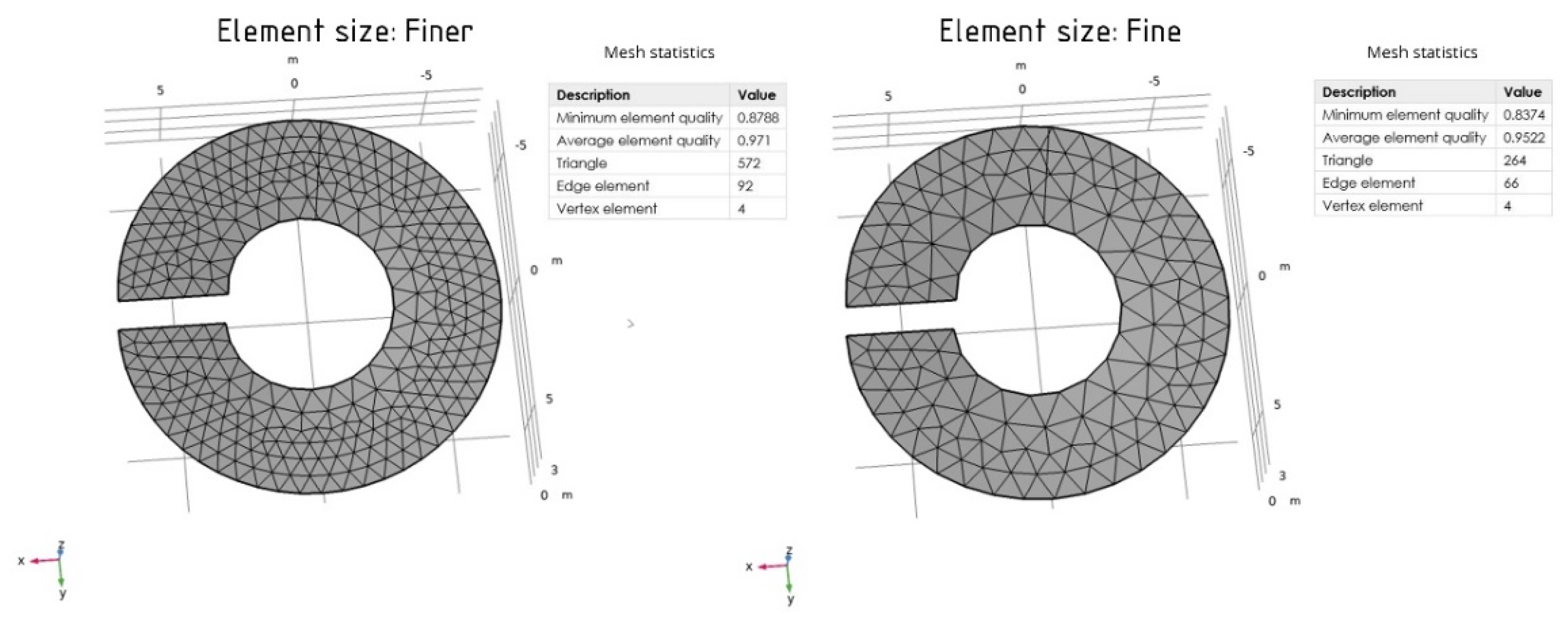
3. As a result of building an automatic mesh, a total of 572 elements is created with the maximum element size of 0.786 m and the minimum element size of 0.0572 m. The thickness of the shell is set to 0.16 m. The fixed constraint is installed on the initial, final, and internal faces of the structure (Figure 7).
Subsequently, the stress–strain analysis is also conducted. On the z-axis, the maximum displacement value is 53.38 mm. The values of the first principal stress are −4.5 × 10⁻¹⁵ MPa (minimum) and 6.9 MPa (maximum). For the second principal stress, the minimum value is −10 MPa and the maximum value is 0.22 MPa. The values of the third principal stress are −34.73 MPa (minimum) and −1.4 × 10⁻¹⁷ MPa (maximum). The total elastic strain energy is 18,283.8 J. Figure 8 represents a graphical diagram showing the maximum and minimum values.
Next, the mesh type is changed from «fine» to «finer» (Figure 9) and the model is split into 264 triangles. The maximum element size is 1.14 m and the minimum element size is 0.143 m.
The maximum displacement value is 53.46 mm. The values of the first principal stress are −1.5 × 10⁻¹⁵ MPa (minimum) and 7.11 MPa (maximum). For the second principal stress, the minimum value is −12.96 MPa and the maximum value is 0.42 MPa. The values of the third principal stress are 3.5 × 10⁻¹⁶ MPa (maximum) and −33.60 MPa (minimum). The total elastic strain energy is 18,339.9 J. The graphical diagram showing the maximum and minimum values is presented in Figure 10.
The shape optimization of the helicoid shell is also carried out using three methods in Comsol. Similar to the conducted research of the sphere as an objective function for optimization, the total elastic strain energy is chosen, and the two control variable settings have the following values: dmax –0.25 m, Rmin = 1 m.

3. Results

3.1. The Optimization of the Sphere Shell (Finer Element Size)

To begin with, the calculation of the spherical dome is carried out using the Sparse Nonlinear OPTimizer or SNOPT.
For the optimized shell on the z-axis, the maximum displacement value is 1.28 mm. The first principal stress has the following values: −7.8 × 10⁻¹⁶ MPa (minimum) and 0.45 MPa (maximum). For the second principal stress, the minimum value is −1.56 MPa and the maximum value is 4.45 MPa. The values of the third principal stress are −0.90 MPa (minimum) and −3.58 MPa (maximum). The normal boundary displacement is 76% and the total elastic energy is 4462 J. The results are shown in Figure 11.
Then, the calculation is carried out using the Interior Point OPTimizer or IPOPT.
On the z-axis, the maximum displacement value is 1.16 mm. The first principal stress has the following values: 1.38 MPa (maximum) and −1.1 × 10⁻¹⁵ MPa (minimum). For the second principal stress, the maximum value is 1.07 MPa and the minimum value is −1.57 MPa. The values of the third principal stress are 5.1 × 10⁻¹⁷ MPa (maximum) and −2.81 MPa (minimum). The normal boundary displacement for the optimized shell is 107% and the total elastic energy is 4157 J. The results are shown in Figure 12.
In the end, the calculation is carried out using the MMA method. For the optimized shell using this method of calculation on the z-axis, the maximum displacement value is 1.73 mm. The first principal stress has he following values: 0.64 MPa (maximum) and −7.4 × 10⁻¹⁶ MPa (minimum). For the second principal stress, the minimum value is −1.60 MPa and the maximum value is 5.5 × 10⁻¹⁶ MPa. The values of the third principal stress are −1.16 MPa (maximum) and −3.45 MPa (minimum). The normal boundary displacement for the optimized shell is 24% and the total elastic energy is 6039 J. The results are shown in Figure 13.
Thus, analyzing the obtained values, it should be noted that all three optimization methods similarly change the shell, gradually compressing it to the center of the sphere. At the same time, the IPOPT method used for the same number of iterations reduces the function to 4157 J, which is lower than in other methods. The shell is also changed the most in this method; the height changes from 10 m to 7 m, which indicates the greatest variability of solutions for the spherical dome. IPOPT shows the highest efficiency, which is characteristic of the algorithms related to an interior-point line-search filter method [20]. By using the SNOPT method, the total elastic energy is reduced to 4462 J. The shell geometry is changed less, but the result achieved by this method on the 50th iteration is similar to what is achieved by the IPOPT method for about 35 iterations. The most minor changes are obtained using the MMA method. With this method, it is possible to achieve only those results that are in the IPOPT method at 25 iterations. Table 1 shows the values of the computational time.
According to the calculation results, the average values of the optimized function for the calculations using the three methods are as follows: 5628.96 J (SNOPT), 5442.41 J (IPOPT), and 6674.92 J (MMA).
As for the total time of the optimization calculation, the fastest result is obtained by using the SNOPT method (Table 1).

3.2. The Optimization of the Sphere Shell (Fine Element Size)

First, the calculations are performed using the SNOPT method. The maximum displacement value is 1.32 mm. The first principal stress has the following values: −9.4 × 10⁻¹⁶ MPa (minimum) and 0.54 MPa (maximum). For the second principal stress, the minimum value is −1.73 MPa and the maximum value is 2.1 × 10⁻¹ MPa. The values of the third principal stress are −3.23 MPa (minimum) and −0.95 MPa (maximum). The normal boundary displacement is 100% and the total elastic energy is 4244 J. The results are shown in Figure 14.
Next, the IPOPT method is used for the calculations. For the optimized shell using this method of calculation on the z-axis, the maximum displacement value is 1.31 mm. As for the stress–strain state, the maximum and minimum first stresses are 0.29 MPa and −1.3 × 10⁻¹⁵ MPa, respectively, the second 0.17 MPa and −2.64 MPa, and the third −2.5 × 10⁻²⁰ MPa and −3.18 MPa. The normal boundary displacement is 102% and the total elastic energy is 4175 J. The graphical diagram showing the maximum and minimum values is presented in Figure 15.
For the optimized shell on the z-axis, the maximum displacement value is 1.58 mm. The first principal stress has he following values: −7.4 × 10⁻¹⁶ MPa (minimum) and 0.64 MPa (maximum). For the second principal stress, the minimum value is −1.53 MPa and the maximum value is 4.5 × 10⁻¹⁶ MPa. The values of the third principal stress are −3.48 MPa (minimum) and −1.40 MPa (maximum). The normal boundary displacement is 28% and the total elastic energy is 5733.98 J. The results are shown in Figure 16.
As in the case of a model formed with a finer mesh element, the IPOPT method reduced the function values more than the other methods.
According to the calculation results, the average values of the optimized function for the calculations using the three methods are as follows: 5403 J (SNOPT), 5230 J (IPOPT), and 6392 J (MMA).
As for the total time of the optimization calculation, the fastest result was also obtained by using the SNOPT method (Table 2). It should also be noted that when choosing a fine element size, the calculations are performed faster when choosing any method. This can be explained by the fact that the second version of the computational model contains fewer element triangles than the first one.

3.3. The Optimization of the Helicoid Shell (Finer Element Size)

When calculating 1 loop of the helicoid, the maximum movement along the z-axis is 10.3 mm. As for the stress–strain state, for example, in the MMA method, the maximum and minimum first stresses are 4.39 MPa and −1.1 × 10⁻¹⁵ MPa, respectively, the second 0.66 MPa and −6.53 MPa, and the third 6.6 × 10⁻¹⁶ MPa and −15.21 MPa. The normal boundary displacement is 94% and the total elastic energy is 3096.29 J (Figure 17).
In other methods, the values, as well as their distributions, practically do not differ (Figure 18 and Figure 19). The optimized shape of the helicoid changes the angle of inclination of the surface relative to the horizontal plane and adds a small stiffening rib in the middle of the shell’s span.
In contrast to the optimization of the spherical dome, the optimization process of one loop of the helicoid has similar results through all three methods; the objective function is reduced to about 3096 J (SNOPT and MMA). The value of the optimized function, using the IPOPT method, has a slight difference of 3095 J. As for the total optimization time, all solvers minimize the function relatively quickly; however, it should be noted that 2 of the 3 methods reach the limit value of the function at 24 (SNOPT) and 30 iterations (MMA). It can be assumed that this is achieved due to the fact that a part of the helicoid is obtained for the calculation. The total time of the optimization of one loop of the helicoid is shown in Table 3.
The average values of the optimized function for the calculations using three methods are as follows: 3463 J (SNOPT), 4050 J (IPOPT), and 3500 J (MMA).

3.4. The Optimization of the Helicoid Shell (Fine Element Size)

With fine element size, the following results are obtained with the use of the MMA method: the maximum movement along the z-axis is 10.5 mm. As for the stress–strain state, the maximum and minimum first stresses are 6.13 MPa and −1.1 × 10⁻¹⁵ MPa, respectively, the second 1.26 MPa and −8.4 MPa, and the third 1.2 × 10⁵ MPa and −14.66 MPa. The normal boundary displacement for the optimized shell is 90% and the total elastic energy is 3223 J. The results are shown in Figure 20.
The calculation is also carried out using the SNOPT and IPOPT methods. The following results are obtained when using the SNOPT method: the maximum movement along the z-axis is 10.5 mm. The maximum and minimum first stresses are 6.22 MPa and −2.3 × 10⁻¹⁵ MPa, respectively, the second 1.32 MPa and −8.33 MPa, and the third 1.3 × 10⁻¹⁶ MPa and −14.48 MPa. The normal boundary displacement for the optimized shell is 91% and the total elastic strain energy is 3223 J (Figure 21).
For the optimized shell using the IPOPT method on the z-axis, the maximum displacement value is 10.6 mm. The values of the first principal stress are 6.15 MPa (maximum) and −1.6 × 10⁻¹⁵ MPa (minimum). For the second principal stress, the maximum value is 1.27 MPa and the minimum value is −8.38 MPa. The values of the third principal stress are 4.3 × 10⁻¹⁶ MPa (maximum) and −14.62 MPa (minimum). The normal boundary displacement for the optimized shell is 90% and the total elastic strain energy is 3223 J. The graphical diagram showing the maximum and minimum values is presented in Figure 22.
In the case of the second variant of the model with a fine element size, the obtained function values are similar in each method. Here, the objective function is reduced to about 3223 (SNOPT and IPOPT). However, the values of the optimized function using the fine mesh, on the contrary, turn out to be larger, unlike the sphere. The same can be said about the total time of the optimization calculation. In this case, the calculations took more time to perform (Table 4). This may be due to the most complex geometry of the model.
The average values of the optimized function for the calculation model with a fine element size using the three methods are as follows: 3540 J (SNOPT), 4100 J (IPOPT), and 3620 J (MMA).

4. Discussion

The present article considers the optimization of the shape of two different shells, the spherical dome and one helicoid loop, with two types of element sizes for each mesh. Even though both tasks are similar to each other, different Comsol optimization methods cope with them in different ways, which allows us to output the following results:
  • In addition to the setting criteria or input parameters, the construction of the mesh has a significant impact on the calculations of simple and complex forms. In the case of the spherical dome, changing the mesh element size from finer to fine leads to a decrease in the total calculation time and to a greater decrease in the value of the objective function. The reverse situation is present in the calculation of the one loop helicoid, from which we can make the assumption that the computational grid has a different effect on shells with different geometries.
  • When solving the spherical dome optimization problem, IPOPT is the most optimal method, while the SNOPT algorithm is only a few iterations short of IPOPT’s result, and the MMA method reduces the objective function twice as ineffectively as IPOPT, significantly lagging behind the other two methods.
  • In relation to the spherical dome, by using shape optimization, it is possible to significantly reduce the objective function by more than twice, as well as the maximum displacement of the shell. In general, the resulting surface is also much less deformed. At the same time, the shell is quite different from the original geometry; the surface corresponds more to a one-sheeted hyperboloid of revolution than to a spherical dome. Based on this, it can be concluded that shells shallower than a sphere are better suited for a round floor structure.
  • When optimizing the helicoid, all three methods show almost the same results for the same number of iterations. Thus, it can be concluded that the choice of the form optimization method depends not only on the essence of the task, but also on the geometry of the model. The objective function is reduced by more than ten times, and the maximum displacement is reduced by five times. The geometry of the shell has not undergone such significant changes. Although the helicoid turns from a straight one into an oblique one (due to the deviation of the surface from the horizontal plane), the most decrease in the objective function is associated with the addition of a stiffening rib to the surface.

5. Conclusions

As a result, the present article shows that optimizing the shape of the shells can significantly reduce the total deformation of the structure. The choice of the optimization method significantly affects the final result, but it depends more on the geometry of the shell and the element size for each mesh. The resulting shape no longer corresponds to the original definition of the surface, but such results show the possibility of further research into optimizing the shape of shells to find the most optimal surfaces when solving general design problems.
It should be noted that, in the Comsol program, optimization can also be carried out according to acoustic criteria, and the design variables are related to the physics of acoustics. The optimization of acoustics is considered in [30]. Future research is planned to be devoted to this topic.

Author Contributions

Conceptualization, E.E. and M.R.; investigation and methodology, E.E. and T.E.; writing—original draft preparation, E.E. and T.E.; supervision, M.R. All authors have read and agreed to the published version of the manuscript.

Funding

This research received no external funding.

Institutional Review Board Statement

Not applicable.

Informed Consent Statement

Not applicable.

Data Availability Statement

Not applicable.

Acknowledgments

This paper was supported by the RUDN University Strategic Academic Leadership Program.

Conflicts of Interest

The authors declare no conflict of interest.

References

  1. Eren, H. Mathematical methods of Optimization. In Handbook of Measuring System Design; Sydenham, P.H., Thorn, R., Eds.; John Wiley & Sons: Hoboken, NJ, USA, 2005; p. 1648. [Google Scholar] [CrossRef]
  2. Sinha, G.R. Modern Optimization Methods for Science, Engineering and Technology; Institute of Physics Publishing: Bristol, UK, 2020; pp. 1–18. [Google Scholar] [CrossRef]
  3. Cavazzuti, M. Optimization Methods: From Theory to Design; Springer: Berlin/Heidelberg, Germany, 2013; p. 257. [Google Scholar]
  4. Haslinger, J.; Mäkinen, R.A.E. Introduction to Shape Optimization: Theory, Approximation, and Computation; SIAM: Philadelphia, PA, USA, 2003. [Google Scholar]
  5. Allaire, G.; Henrot, A. On some recent advances in shape optimization. Comptes Rendus de l’Académie des Sciences-Series IIB-Mechanics 2001, 329, 383–396. [Google Scholar] [CrossRef]
  6. Souza, M.; Pauletti, R.M. Parametric design and optimization of shell structures using the Natural Force Density Method. In Proceedings of the IASS Annual Symposium “Spatial Structures in the 21st Century”, Tokyo, Japan, 26–30 September 2016. [Google Scholar]
  7. Sassone, M.; Pugnale, A. Evolutionary Structural Optimization in Shells Design. Adv. Numer. Anal. Shell-Like Struct. 2007, 4, 247–257. [Google Scholar]
  8. Omid, H.; Golabchi, M. Survey of parametric optimization plugins in Rhinoceros used in contemporary architectural design. In Proceedings of the Fourth International Conference on Modern Research in Civil Engineering, Architecture, Urban Management and Environment, Karaj, Iran, 17 December 2020. [Google Scholar]
  9. Cui, G. Shape optimization based on ANSYS. J. Inf. Comput. Sci. 2015, 12, 4291–4297. [Google Scholar] [CrossRef]
  10. Seranaj, A.; Elezi, E.; Seranaj, A. Structural optimization of reinforced concrete spatial structures with different structural openings and forms. Res. Eng. Struct. Mater. 2018, 4, 79–89. [Google Scholar] [CrossRef]
  11. Mekjavić, I.; Pičulin, S. Structural analysis and optimization of concrete spherical and groined shells. Teh. Vjesn. 2010, 17, 537–544. [Google Scholar]
  12. Fossen, S.M.B. Parallel Computing and Optimization with COMSOL Multiphysics. Master’s Thesis, Norwegian University of Science and Technology, Trondheim, Norway, 2017. [Google Scholar]
  13. Slawig, T.; Prüfert, U. Mathematics-based Optimization in the Comsol Multiphysics Framework. In Proceedings of the Comsol User Conference, Stuttgart, Germany, 26–28 October 2011. [Google Scholar]
  14. Hashim, A.A.; Mahmoud, K.I.; Ridha, H. Geometry and shape optimization of piezoelectric cantilever energy harvester using COMSOL multiphysics software. Int. Rev. Appl. Sci. Eng. 2021, 12, 103–110. [Google Scholar] [CrossRef]
  15. Svanberg, K. The method of moving asymptotes-a new method for structural optimization. Int. J. Numer. Methods Eng. 1987, 24, 359–373. [Google Scholar] [CrossRef]
  16. Svanberg, K. A class of globally convergent optimization methods based on conservative convex separable approximations. SIAM J. Optim. 2002, 12, 555–573. [Google Scholar] [CrossRef] [Green Version]
  17. Svanberg, K. MMA and GCMMA—Fortran Versions; KTH, Royal Institute of Technology: Stockholm, Sweden, 2013. [Google Scholar]
  18. Fanni, M.; Shabara, N.; Alkalla, M.A. Comparison Between Different Topology Optimization Methods. Eng. J. 2013, 38, 13–24. [Google Scholar] [CrossRef]
  19. Bruyneel, M.; Duysinx, P.; Fleury, C. A family of MMA approximations for structural optimization. Struct. Multidiscip. Optim. 2002, 24, 263–276. [Google Scholar] [CrossRef] [Green Version]
  20. Leyffer, S.; Mahajan, A. Nonlinear Constrained Optimization: Methods and Software; Argonne National Laboratory: Lemont, IL, USA, 2010; pp. 1–24. [Google Scholar]
  21. Yu, Y.; Lyu, Z.; Xu, Z.; Martins, J.R. On the Influence of Optimization Algorithm and Starting Design on Wing Aerodynamic Shape Optimization. Aerosp. Sci. Technol. 2018, 75, 183–199. [Google Scholar] [CrossRef]
  22. Gill, P.E.; Murray, W.; Saunders, M.A. SNOPT: An SQP Algorithm for Large-scale Constrained Optimization. SIAM J. Optim. 2002, 12, 979–1006. [Google Scholar] [CrossRef] [Green Version]
  23. Wächter, A. Short Tutorial: Getting Started with Ipopt in 90 Minutes. In Proceedings of the Dagstuhl Seminar, Dagstuhl, Germany, 8–11 February 2009; pp. 1–17. [Google Scholar]
  24. Krivoshapko, S.N. Optimal shells of revolution and main optimizations. Struct. Mech. Eng. Constr. Build. 2019, 15, 201–209. [Google Scholar] [CrossRef] [Green Version]
  25. Hinz, M.; Magoulès, F.; Rozanova-Pierrat, A.; Rynkovskaya, M.; Teplyaev, A. On the existence of optimal shapes in architecture. Appl. Math. Model. 2020, 94, 676–687. [Google Scholar] [CrossRef]
  26. Rynkovskaya, M.I.; Elberdov, T.; Sert, E.; Öchsner, A. Study of modern software capabilities for complex shell Analysis. Struct. Mech. Eng. Constr. Build. 2020, 16, 45–53. [Google Scholar] [CrossRef]
  27. Bui, V.P.; Prokopov, V.S.; Gavriushin, S.S.; Papazafeiropoulos, G. Topology Optimization of the Turbine Disk Structure under Thermomechanical Loads. Izv. Vyss. Uchebnyh Zavedenij Mashinostroenie 2019, 4, 60–70. [Google Scholar] [CrossRef]
  28. Krivoshapko, S.N.; Ivanov, V.N. Encyclopedia of Analytical Surfaces; Springer International Publishing: Cham, Switzerland, 2015; p. 457. [Google Scholar] [CrossRef]
  29. Rynkovskaya, M.I.; Ivanov, V.N. Analytical method to analyze right helicoid stress-strain. In Engineering Design Applications, Adv Struct Mater; Öchsner, A., Altenbach, H., Eds.; Springer International Publishing: Cham, Switzerland, 2019; Volume 92, pp. 157–171. [Google Scholar] [CrossRef]
  30. Echenagucia, T.M.; Block, P. Acoustic optimization of funicular shells. In Proceedings of the International Association for Shell and Spatial Structures (IASS), Amsterdam, The Netherlands, 17–20 August 2015. [Google Scholar]
Figure 1. The necessary components of optimization.
Computation 10 00054 g001
Figure 2. The necessary components of optimization.
Computation 10 00054 g002
Figure 3. Scheme of preparation of the sphere shell for calculation.
Computation 10 00054 g003
Figure 4. The structural analysis of the sphere shell (finer element size).
Computation 10 00054 g004
Figure 5. The use of two element sizes for the mesh.
Computation 10 00054 g005
Figure 6. The structural analysis of the sphere shell (fine element size).
Computation 10 00054 g006
Figure 7. Scheme of preparation of the sphere shell for calculation.
Computation 10 00054 g007
Figure 8. The structural analysis of the helicoid shell (finer element size).
Computation 10 00054 g008
Figure 9. The use of two element sizes for the mesh.
Computation 10 00054 g009
Figure 10. The structural analysis of the helicoid shell (fine element size).
Computation 10 00054 g010
Figure 11. The results of the optimized shell using the SNOPT method.
Computation 10 00054 g011
Figure 12. The results of the optimized shell using the IPOPT method.
Computation 10 00054 g012
Figure 13. The results of the optimized shell using the MMA method.
Computation 10 00054 g013
Figure 14. The results of the optimized shell using the SNOPT method.
Computation 10 00054 g014
Figure 15. The results of the optimized shell using the IPOPT method.
Computation 10 00054 g015
Figure 16. The results of the optimized shell using the MMA method.
Computation 10 00054 g016
Figure 17. The results of the optimized shell using the MMA method.
Computation 10 00054 g017
Figure 18. The results of the optimized shell using the SNOPT method.
Computation 10 00054 g018
Figure 19. The results of the optimized shell using the IPOPT method.
Computation 10 00054 g019
Figure 20. The results of the optimized shell using the MMA method.
Computation 10 00054 g020
Figure 21. The results of the optimized shell using the SNOPT method.
Computation 10 00054 g021
Figure 22. The results of the optimized shell using the IPOPT method.
Computation 10 00054 g022
Table 1. Computational times for the three optimizers.
OptimizerOptimized Function (J) on the 50th IterationTotal Computation Time (s)
SNOPT44622742
IPOPT41575682
MMA603911,010
Table 2. Computational times for the three optimizers.
OptimizerOptimized Function (J) on the 50th IterationTotal Computation Time (s)
SNOPT42442659
IPOPT41754940
MMA57346314
Table 3. Computational times for the three optimizers.
OptimizerIterationsOptimized Function (J)Total Computation Time (s)
SNOPT243096980
IPOPT5030951093
MMA3030961627
Table 4. Computational times for the three optimizers.
OptimizerIterationsOptimized Function (J)Total Computation Time (s)
SNOPT2632231541
IPOPT3732233215
MMA2432242551
Publisher’s Note: MDPI stays neutral with regard to jurisdictional claims in published maps and institutional affiliations.

