Closed-Form Formula for the Conditional Moments of Log Prices under the Inhomogeneous Heston Model

Abstract

Several financial instruments have been thoroughly calculated via the price of an underlying asset, which can be regarded as a solution of a stochastic differential equation (SDE), for example the moment swap and its exotic types that encourage investors in markets to trade volatility on payoff and are especially beneficial for hedging on volatility risk. In the past few decades, numerous studies about conditional moments from various SDEs have been conducted. However, some existing results are not in closed forms, which are more difficult to apply than simply using Monte Carlo (MC) simulations. To overcome this issue, this paper presents an efficient closed-form formula to price generalized swaps for discrete sampling times under the inhomogeneous Heston model, which is the Heston model with time-parameter functions. The obtained formulas are based on the infinitesimal generator and solving a recurrence relation. These formulas are expressed in an explicit and general form. An investigation of the essential properties was carried out for the inhomogeneous Heston model, including conditional moments, central moments, variance, and skewness. Moreover, the closed-form formula obtained was numerically validated through MC simulations. Under this approach, the computational burden was significantly reduced.

1. Introduction

The Heston model [1] is a diffusion model that consists of two stochastic processes, where the dynamics of the first process involve the instantaneous variance process, namely the Cox–Ingersoll–Ross (CIR) process [2]. The model can be applied to basic derivative products with various prices and allows the instantaneous variance to be the CIR process having its mean reversion. The Heston model appears in a wide variety of real-world applications in different branches of mathematical science; see [1,3,4,5,6] for more details. For example, a well-known application of the Heston model is the variance swap pricing based on log prices; see [7,8,9,10,11]. The model can be also applied to the energy industry as financial applications; see [12,13,14] for more details. In the variance swap context observed by Zhu and Lian [9], two main types of swap valuation approaches exist, numerical and analytical methods. However, the numerical method increases the computational burden. In contrast, the analytical method is poorly studied in general. Investigating the Heston model’s properties is still challenging.

Commonly, the CIR process is applied to describe the dynamics of the interest rates or instantaneous variance in the Heston model of the stochastic interest rate or stochastic volatility models. In practice, strong empirical evidence shows that the movements in practice tend to involve time; see [15,16,17,18,19]; thus, the dynamics of the processes are usually governed by time parameters. In the case of the CIR process, it becomes the extended CIR (ECIR) process [16], which has been investigated in numerous research works such as [16,17], who studied an extension of the CIR process that is more suitable for the data than the CIR process. In 2011, Grzelak and Oosterlee [20] discussed an extension of the Heston model by replacing the constant interest rate by a stochastic environment. However, the properties of the process, such as conditional moments, central moments, and variance, are rarely investigated. In this study, we call the Heston model with time-parameter functions the inhomogeneous Heston model. Unlike the Heston model, the conditional moments and properties of the inhomogeneous Heston model cannot be derived directly by using the transition probability density function (PDF) due to the arbitrary time-parameter functions in the process that make the transition PDFs unknown.

Under sufficient conditions, this research provides a closed-form formula for the conditional moments of log prices under the inhomogeneous Heston model. Based on a partial differential equation (PDE) according to the infinitesimal generator [21], a recursive coefficient function was obtained. The obtained formula was derived by solving the PDE without requiring any knowledge of the transition PDFs. The presented formula is more general in terms of time-dependent parameters than other approaches in the literature. Some essential properties of the inhomogeneous Heston model are observed, which can be beneficial for statistical applications, such as for calculating the variance swap valuation, which is also more general in terms of the time-dependent parameters than Zhu and Lian’s results [9].

The rest of the paper is organized as follows: Section 2 provides a brief overview of the Heston model and the inhomogeneous Heston model. Section 3 mentions the main methodology to address the relevant concepts for our proposed results, which are closed-form formulas for the conditional moments of the inhomogeneous Heston model. Section 4 provides the essential properties of the closed-form formula. Section 5 experimentally validates our proposed formulas for the inhomogeneous Heston model for time-inhomogeneous cases via Monte Carlo (MC) simulations. Section 6 concludes the paper.

2. Inhomogeneous Heston Model

The original Heston model was first introduced by Heston [1] for application to option pricing, which satisfies the dynamics of the following stochastic differential equations (SDEs):

$$\left\{\begin{array}{cc}\hfill d{S}_t& =r{S}_{t}dt+\sqrt{v_t}{S}_{t}d{\tilde{W}}_t^S,\hfill \\ \hfill d{v}_t& =\kappa (\theta -v_t)dt+\sigma \sqrt{v_t}d{\tilde{W}}_t^v,\hfill \end{array}\right.$$

(1)

where $S_t$ is the price of the asset at time t, r is a constant interest rate of the asset, $v_t$ is a stochastic instantaneous variance, $\theta$ is the long-term average of variance of the price, $\kappa$ is the rate of reverting to $\theta$, $\sigma$ is the volatility of volatility, and $d{\tilde{W}}_t^S$ and $d{\tilde{W}}_t^v$ are two Winner processes. The stochastic instantaneous variance in the Heston model can be represented by the CIR process [2].

In 2011, Grzelak and Oosterlee [20] discussed an extension of the Heston model, replacing constant interest rate r by time-dependent interest rate $r\left(t\right)$. In addition, References [16,17,18] studied an extension of the CIR process, which is more suitable for the data than the CIR process. Consequently, we considered an extended Heston model by using $r\left(t\right)$ and a general form of the ECIR that appeared in [18] to describe the stochastic instantaneous variance and having a general form as follows:

$$\left\{\begin{array}{cc}\hfill d{S}_t& =r\left(t\right)S_{t}dt+\sqrt{v_t}{S}_{t}d{\tilde{W}}_t^S,\hfill \\ \hfill d{v}_t& =\kappa \left(t\right)(\theta \left(t\right)-v_t)dt+\sigma \left(t\right)\sqrt{v_t}d{\tilde{W}}_t^v,\hfill \end{array}\right.$$

(2)

where $\theta \left(t\right)$ and $\kappa \left(t\right)$ are smooth and bounded time-dependent parameter functions; $d{\tilde{W}}_t^S$ and $d{\tilde{W}}_t^v$ are correlated Winner processes with correlation coefficient $\rho$ based on a filtered probability space $(\mathsf{\Omega },{\mathcal{F}}_t,{\left\{{\mathcal{F}}_t\right\}}_{0\le t\le T},Q)$ generated by an adapted the Brownian motion ${\tilde{W}}_t^S$ and ${\tilde{W}}_t^v$, where $\mathsf{\Omega }$ is a sample space, Q is a risk-neutral measure, and the family ${\left\{{\mathcal{F}}_t\right\}}_{0\le t\le T}$ of the $\sigma$-field on $\mathsf{\Omega }$ parametrized over $t\in [0,T]$ is a filtration. By applying Itô’s lemma [21] with $x_t:=ln{S}_t$ for all $t\ge 0$ to the first equation of (2), the process for the log price can be rewritten as:

$$d{x}_t=\frac{d{S}_t}{S_t}-\frac{1}{2}{\left(\frac{d{S}_t}{S_t}\right)}^2=\left(r\left(t\right)-\frac{1}{2}{v}_t\right)dt+\sqrt{v_t}d{\tilde{W}}_t^S.$$

Then, the system (2) becomes:

$$\left\{\begin{array}{c}d{x}_t=\left(r\left(t\right)-\frac{1}{2}{v}_t\right)dt+\sqrt{v_t}d{\tilde{W}}_t^S,\hfill \\ d{v}_t=\kappa \left(t\right)(\theta \left(t\right)-v_t)dt+\sigma \left(t\right)\sqrt{v_t}d{\tilde{W}}_t^v.\hfill \\ d{\tilde{W}}_t^{S}d{\tilde{W}}_t^v=\rho dt.\hfill \end{array}\right.$$

(3)

To obtain a dynamical system with mutually independent Winner processes $W_t^S$ and $W_t^v$, by applying the Cholesky decomposition method [22] with the system (3), the system (3) can be rewritten as:

$$\left[\begin{array}{c}d{x}_t\\ d{v}_t\end{array}\right]=\left[\begin{array}{c}r\left(t\right)-\frac{1}{2}{v}_t\\ \kappa \left(t\right)(\theta \left(t\right)-v_t)\end{array}\right]dt+\mathsf{\Sigma }C\left[\begin{array}{c}{W}_t^S\\ W_t^v\end{array}\right],$$

where matrices $\mathsf{\Sigma }$ and C are defined by:

$$\mathsf{\Sigma }=\left[\begin{array}{cc}\sqrt{v_t}& 0\\ 0& \sigma \left(t\right)\sqrt{v_t}\end{array}\right]\mathrm{and}C=\left[\begin{array}{cc}1& 0\\ \rho & \sqrt{1-{\rho }^2}\end{array}\right]\mathrm{satisfying}C{C}^{\top }=\left[\begin{array}{cc}1& \rho \\ \rho & 1\end{array}\right],$$

and Winner processes $W_t^S$ and $W_t^v$ are mutually independent under $\mathbb{Q}$ satisfying:

$$\left[\begin{array}{c}d{\tilde{W}}_t^S\\ d{\tilde{W}}_t^v\end{array}\right]=C\left[\begin{array}{c}d{W}_t^S\\ d{W}_t^v\end{array}\right].$$

Finally, the dynamical system (3) becomes:

$$\left\{\begin{array}{cc}\hfill d{x}_t& =\left(r\left(t\right)-\frac{1}{2}{v}_t\right)dt+\sqrt{v_t}d{W}_t^S,\hfill \\ \hfill d{v}_t& =\kappa \left(t\right)(\theta \left(t\right)-v_t)dt+\rho \sigma \left(t\right)\sqrt{v_t}d{W}_t^S+\sigma \left(t\right)\sqrt{v_t}\sqrt{1-{\rho }^2}d{W}_t^v.\hfill \end{array}\right.$$

(4)

To ensure that a pathwise unique strong solution exists for the ECIR process $v_t$ given in (4) and to avoid zero a.s. with respect to the measure Q for all $t\in [0,T]$, the two assumptions below proposed by Maghsoodi [17], Rogers and Williams [23], and Ekström et al. [24] are required.

Assumption 1.

The functions $\theta \left(t\right),\kappa \left(t\right)$, and $\sigma \left(t\right)$ in the ECIR process $v_t$ given in (4) are strictly positive, smooth, and continuous time-dependent functions on $[0,T]$. Moreover, the ECIR process $v_t$ holds the inequality $2\kappa \left(t\right)\theta \left(t\right)>\sigma {\left(t\right)}^2$.

According to Assumption 1, this paper defines the parameter function space of the inhomogeneous Heston model (4) as follows:

$$\left\{\left(r\left(t\right),\kappa \left(t\right),\theta \left(t\right),\sigma \left(t\right),\tau ,\rho \right)\in {\left({\mathbb{R}}^{+}\right)}^5\times [-1,1]\mid 2\kappa \left(t\right)\theta \left(t\right)>\sigma {\left(t\right)}^2\right\}$$

(5)

for all $t\in [0,T]$ where $\tau =T-t\ge 0$.

Under Assumption 1 and the parameter space (5), this study proposes a closed-form formula for log prices on the basis of the inhomogeneous Heston model (4), where the parameters depend on time, in the form:

$${\mathbf{E}}^Q\left[x_T^n\mid {\mathcal{F}}_t\right]={\mathbf{E}}^Q\left[x_T^n\mid \left(x_t=x,v_t=v\right)\right]:={\mathbf{E}}_t^Q\left[x_T^n\right],0\le t\le T,$$

(6)

for the degree $n\in \mathbb{N}$. The idea of our results relies on a solution of the PDE given in the infinitesimal generator for a two-dimensional diffusion process [21], which corresponds to the solution of (6). Roughly speaking, by expressing the solution of the PDE as a polynomial expression, we can solve its coefficients to obtain a closed-form formula directly. The motivation for the form of conditional moments, that is a solution to the PDE, is based on [25,26,27,28,29]; considering that both SDEs in the inhomogeneous Heston model (4) have linear drift and linear squared diffusion coefficients, the infinitesimal generator maps polynomials to polynomials; see more details in [25,26,30,31].

3. Main Results

This section presents a closed-form formula for the conditional moments corresponding to the two-factor model (4) based on the solution of the PDE according to the infinitesimal generator for the two-dimensional diffusion process [21]. The formula is provided in Theorem 1 as function $u^{\left(n\right)}(x,v,\tau ):={\mathbf{E}}_t^Q\left[x_T^n\right]$. Next, we derive a formula for the first conditional moment of log price $x_t$ as a consequence of Theorem 1, which is represented in Corollary 1.

Theorem 1.

Suppose that $n\ge 2$ is an integer and $S_t$ follows the dynamics described by the inhomogeneous Heston model (4), then:

$$u^{\left(n\right)}(x,v,\tau )=\sum _{j=0}^n\sum _{\ell =0}^j{A}_{j,\ell }^{\left(n\right)}\left(\tau \right)x^{\ell }{v}^{j-\ell },$$

(7)

where $\tau =T-t\ge 0$, $(x,v)\in \mathbb{R}\times {\mathbb{R}}^{+}$, and $A_{j,\ell }^{\left(n\right)}\left(\tau \right)$ can be obtained by solving the system of recursive ordinary differential equations (ODEs), for all $0\le \ell \le j\le n$,

$$\begin{array}{cc}\hfill {\displaystyle \frac{d}{d\tau }}{A}_{n,n}^{\left(n\right)}\left(\tau \right)& =0,\hfill \end{array}$$

(8)

$$\begin{array}{cc}\hfill {\displaystyle \frac{d}{d\tau }}{A}_{n,b}^{\left(n\right)}\left(\tau \right)& =-{\displaystyle \frac{1}{2}}(b+1)A_{n,b+1}^{\left(n\right)}\left(\tau \right)-\kappa (T-\tau )(n-b)A_{n,b}^{\left(n\right)}\left(\tau \right)\mathrm{for}0\le b\le n-1,\hfill \end{array}$$

(9)

$$\begin{array}{cc}\hfill {\displaystyle \frac{d}{d\tau }}{A}_{a,a}^{\left(n\right)}\left(\tau \right)& =r(T-\tau )(a+1)A_{a+1,a+1}^{\left(n\right)}\left(\tau \right)+\kappa (T-\tau )\theta (T-\tau )A_{a+1,a}^{\left(n\right)}\left(\tau \right)\mathrm{for}1\le a\le n-1,\hfill \\ \hfill {\displaystyle \frac{d}{d\tau }}{A}_{a,b}^{\left(n\right)}\left(\tau \right)& ={\displaystyle \frac{1}{2}}(b+2)(b+1)A_{a+1,b+2}^{\left(n\right)}\left(\tau \right)\hfill \\ \hfill & +\left({\displaystyle \frac{1}{2}}{\sigma }^2(T-\tau )((a+1)-b)(a-b)+\kappa (T-\tau )\theta (T-\tau )((a+1)-b)\right)A_{a+1,b}^{\left(n\right)}\left(\tau \right)\hfill \\ \hfill & +\left(\rho \sigma (T-\tau )(b+1)(a-b)+r(T-\tau )(b+1)\right)A_{a+1,b+1}^{\left(n\right)}\left(\tau \right)-{\displaystyle \frac{1}{2}}(b+1)A_{a,b+1}^{\left(n\right)}\left(\tau \right)\hfill \end{array}$$

(10)

$$\begin{array}{cc}\hfill & -\kappa (T-\tau )(a-b)A_{a,b}^{\left(n\right)}\left(\tau \right),\mathrm{for}1\le b+1\le a\le n-1,\mathrm{and}\hfill \end{array}$$

(11)

$$\begin{array}{cc}\hfill {\displaystyle \frac{d}{d\tau }}{A}_{0,0}^{\left(n\right)}\left(\tau \right)& =r(T-\tau )A_{1,1}^{\left(n\right)}\left(\tau \right)+\kappa (T-\tau )\theta (T-\tau )A_{1,0}^{\left(n\right)}\left(\tau \right)\hfill \end{array}$$

(12)

subject to the initial conditions $A_{n,n}^{\left(n\right)}\left(0\right)=1$ and $A_{a,b}^{\left(n\right)}\left(0\right)=0$ for $0\le b\le a\le n-1$.

Proof. 

From Appendix A of Rujivan and Zhu [32], we obtain the PDE associated with the Heston model (2) when $x_t=ln{S}_t$ as follows:

$$\begin{array}{cc}\hfill -\frac{\partial u^{\left(n\right)}}{\partial \tau }+\frac{1}{2}v\frac{{\partial }^2{u}^{\left(n\right)}}{\partial x^2}& +\frac{1}{2}{\sigma }^2\left(t\right)v\frac{{\partial }^2{u}^{\left(n\right)}}{\partial v^2}+\rho \sigma \left(t\right)v\frac{{\partial }^2{u}^{\left(n\right)}}{\partial x\partial v}\hfill \\ \hfill & +\left(r\left(t\right)-\frac{1}{2}v\right)\frac{\partial u^{\left(n\right)}}{\partial x}+\kappa \left(t\right)(\theta \left(t\right)-v)\frac{\partial u^{\left(n\right)}}{\partial v}=0\hfill \end{array}$$

(13)

which are subject to the terminal condition:

$$\begin{array}{c}\hfill u^{\left(n\right)}(x,v,0)=x^n\end{array}$$

(14)

for all $(x,v)\in \mathbb{R}\times {\mathbb{R}}^{+}$. Let $\tau =T-t>0$. We solve the PDE (13) subject to the terminal condition (14) by assuming that the solution can be written in the form:

$$\begin{array}{c}\hfill u^{\left(n\right)}(x,v,t)=\sum _{j=0}^n\sum _{\ell =0}^j{A}_{j,\ell }^{\left(n\right)}\left(\tau \right)x^{\ell }{v}^{j-\ell }\end{array}$$

(15)

where $A_{j,\ell }^{\left(n\right)}\left(\tau \right)$ is the function depending on $\tau$ for $0\le \ell \le j\le n$. Calculating all partial derivatives of $u^{\left(n\right)}$ in (13) by using the solution form (15) and shifting index gives the relations:

$$\begin{array}{cc}\hfill & \frac{\partial u^{\left(n\right)}}{\partial \tau }=\frac{d{A}_{0,0}^{\left(n\right)}}{d\tau }+\sum _{j=1}^{n-1}\sum _{\ell =0}^{j-1}{x}^{\ell }{v}^{j-\ell }\frac{d{A}_{j,\ell }^{\left(n\right)}}{d\tau }+\sum _{j=1}^{n-1}{x}^j\frac{d{A}_{j,j}^{\left(n\right)}}{d\tau }+\sum _{\ell =0}^{n-1}{x}^{\ell }{v}^{n-\ell }\frac{d{A}_{n,\ell }^{\left(n\right)}}{d\tau }+x^n\frac{d{A}_{n,n}^{\left(n\right)}}{d\tau },\hfill \end{array}$$

(16)

$$\begin{array}{cc}\hfill & \frac{1}{2}v\frac{{\partial }^2{u}^{\left(n\right)}}{\partial x^2}=\sum _{j=1}^{n-1}\sum _{\ell =0}^{j-1}\frac{1}{2}(\ell +2)(\ell +1)x^{\ell }{v}^{j-\ell }{A}_{j+1,\ell +2}^{\left(n\right)},\hfill \end{array}$$

(17)

$$\begin{array}{cc}\hfill & \frac{1}{2}{\sigma }^2(T-\tau )v\frac{{\partial }^2{u}^{\left(n\right)}}{\partial v^2}=\sum _{j=1}^{n-1}\sum _{\ell =0}^{j-1}\frac{1}{2}{\sigma }^2(T-\tau )((j+1)-\ell )(j-\ell )x^{\ell }{v}^{j-\ell }{A}_{j+1,\ell }^{\left(n\right)},\hfill \end{array}$$

(18)

$$\begin{array}{cc}\hfill & \rho \sigma (T-\tau )v\frac{{\partial }^2{u}^{\left(n\right)}}{\partial x\partial v}{v}^{j-(\ell +1)}{A}_{j,\ell }^{\left(n\right)}=\sum _{j=1}^{n-1}\sum _{\ell =0}^{j-1}\rho \sigma (T-\tau )(\ell +1)(j-\ell )x^{\ell }{v}^{j-\ell }{A}_{j+1,\ell +1}^{\left(n\right)},\hfill \\ \hfill & r(T-\tau )\frac{\partial u^{\left(n\right)}}{\partial x}=r(T-\tau )A_{1,1}^{\left(n\right)}+\sum _{j=1}^{n-1}\sum _{\ell =0}^{j-1}r(T-\tau )(\ell +1)x^{\ell }{v}^{j-\ell }{A}_{j+1,\ell +1}^{\left(n\right)}\hfill \end{array}$$

(19)

$$\begin{array}{cc}\hfill & +\sum _{j=1}^{n-1}r(T-\tau )(j+1)x^j{A}_{j+1,j+1}^{\left(n\right)},\hfill \end{array}$$

(20)

$$\begin{array}{cc}\hfill & \frac{1}{2}v\frac{\partial u^{\left(n\right)}}{\partial x}=\sum _{j=1}^{n-1}\sum _{\ell =0}^{j-1}\frac{1}{2}(\ell +1)x^{\ell }{v}^{j-\ell }{A}_{j,\ell +1}^{\left(n\right)}+\sum _{\ell =0}^{n-1}\frac{1}{2}(\ell +1)x^{\ell }{v}^{n-\ell }{A}_{n,\ell +1}^{\left(n\right)},\hfill \\ \hfill & \kappa (T-\tau )\theta (T-\tau )\frac{\partial u^{\left(n\right)}}{\partial v}=\kappa (T-\tau )\theta (T-\tau )A_{1,0}^{\left(n\right)}\hfill \end{array}$$

(21)

$$\begin{array}{cc}\hfill & +\sum _{j=1}^{n-1}\sum _{\ell =0}^{j-1}\kappa (T-\tau )\theta (T-\tau )((j+1)-\ell )x^{\ell }{v}^{j-\ell }{A}_{j+1,\ell }^{\left(n\right)}+\sum _{j=1}^{n-1}\kappa (T-\tau )\theta (T-\tau )x^j{A}_{j+1,j}^{\left(n\right)},\hfill \end{array}$$

(22)

and:

$$\begin{array}{cc}\hfill \kappa (T-\tau )v\frac{\partial u^{\left(n\right)}}{\partial v}& =\sum _{j=1}^{n-1}\sum _{\ell =0}^{j-1}\kappa (T-\tau )(j-\ell )x^{\ell }{v}^{j-\ell }{A}_{j,\ell }^{\left(n\right)}+\sum _{\ell =0}^{n-1}\kappa (T-\tau )(n-\ell )x^{\ell }{v}^{n-\ell }{A}_{n,\ell }^{\left(n\right)}.\hfill \end{array}$$

(23)

Substituting (16)–(23) in (13) and comparing the coefficients of $x^{\ell }{v}^{j-\ell }$ for $0\le \ell \le j\le n$ provide the system of recursive ODEs shown in (8)–(12), as required.    □

Corollary 1.

Suppose that $S_t$ follows the dynamics described by the inhomogeneous Heston model (4), then:

$$u^{\left(1\right)}(x,v,\tau )=\sum _{j=0}^1\sum _{\ell =0}^j{A}_{j,\ell }^{\left(1\right)}\left(\tau \right)x^{\ell }{v}^{j-\ell }$$

(24)

where $\tau =T-t\ge 0$, $(x,v)\in \mathbb{R}\times {\mathbb{R}}^{+}$, and $A_{j,\ell }^{\left(n\right)}\left(\tau \right)$ can be obtained by solving the system of recursive ODEs, for all $0\le \ell \le j\le n$,

$$\begin{array}{cc}\hfill & {\displaystyle \frac{d}{d\tau }}{A}_{1,1}^{\left(1\right)}\left(\tau \right)=0,\hfill \\ \hfill & {\displaystyle \frac{d}{d\tau }}{A}_{1,0}^{\left(1\right)}\left(\tau \right)=-{\displaystyle \frac{1}{2}}{A}_{1,1}^{\left(1\right)}\left(\tau \right)-\kappa (T-\tau )A_{1,0}^{\left(1\right)}\left(\tau \right),\hfill \\ \hfill & {\displaystyle \frac{d}{d\tau }}{A}_{0,0}^{\left(1\right)}\left(\tau \right)=r(T-\tau )A_{1,1}^{\left(1\right)}\left(\tau \right)+\kappa (T-\tau )\theta (T-\tau )A_{1,0}^{\left(1\right)}\left(\tau \right)\hfill \end{array}$$

(25)

which are subject to the initial conditions $A_{1,1}^{\left(1\right)}\left(0\right)=1$ and $A_{1,0}^{\left(1\right)}\left(0\right)=A_{0,0}^{\left(1\right)}\left(0\right)=0$.

Proof. 

We can follow the proof of Theorem 1 when $n=1$ and use the fact that:

$$\frac{{\partial }^2{u}^{\left(1\right)}}{\partial x^2}=\frac{{\partial }^2{u}^{\left(1\right)}}{\partial v^2}=\frac{{\partial }^2{u}^{\left(1\right)}}{\partial x\partial v}=0$$

to complete the proof.    □

Note that our proposed results in this section are more general than other results in the existing literature [7,8,9,10,11,33,34]. Unlike the methods proposed in [7,8,9,10,11,33,34], our method is based on the PDE generated from the infinitesimal generator for the two-dimensional diffusion process, which attempts to assume the solution of the infinitesimal generator in the form of a combination of polynomial expansions between $x_t$ and $v_t$.

One primary concern when we work with the inhomogeneous Heston model (4) is that (8)–(12) and (25) may be indirectly evaluated as exact solutions. Therefore, the conditional moment (7) cannot be expressed as an exact formula. To overcome this issue, a numerical integration method is required, for example, the simple and well-known methods, such as the trapezoidal rule and Simpson’s rule, or higher accuracy methods, such as the Chebyshev integration method [35,36,37], which has been illustrated to produce a much higher accuracy than the other mentioned integration methods when using the same discretizing nodes.

4. Mathematical Properties

This section provides the benefits of all our results in Section 3, such as the first and second conditional moments, conditional variance, conditional central moments, and conditional skewness for the log price $x_t$ of the two-factor model (4) with piecewise constant parameters. Then, we can solve the system of recursive ODEs; see more details in [38].

4.1. First Conditional Moment

By applying Corollary 1, the first conditional moment of the log price based on the Heston model, (4) with $\kappa \left(t\right)=k$, $\theta \left(t\right)=\theta$, and $\sigma \left(t\right)=\sigma$, can be expressed as:

$$\begin{array}{c}\hfill {\mathbf{E}}_t^Q\left[x_T\right]=u^{\left(1\right)}(x,v,\tau )=A_{0,0}^{\left(1\right)}\left(\tau \right)+A_{1,0}^{\left(1\right)}\left(\tau \right)v+A_{1,1}^{\left(1\right)}\left(\tau \right)x,\end{array}$$

where $\tau =T-t$, and solving the initial value problem given in Theorem 1 yields:

$$\begin{array}{cc}\hfill A_{1,1}^{\left(1\right)}\left(\tau \right)& =1,\hfill \\ \hfill A_{1,0}^{\left(1\right)}\left(\tau \right)& =-\frac{1}{2\kappa }{e}^{-\kappa \tau }\left(e^{\kappa \tau }-1\right),\hfill \\ \hfill A_{0,0}^{\left(1\right)}\left(\tau \right)& =-\frac{1}{2\kappa }{e}^{-\kappa \tau }\left(\theta -\theta e^{\kappa \tau }-2r\kappa \tau e^{\kappa \tau }+\theta \kappa \tau e^{\kappa \tau }\right).\hfill \end{array}$$

Remark 1.

The recursive coefficient functions of the first conditional moment in our result agree with the result in Proposition 2.3 of Rujivan and Zhu [32] by comparing $A_{0,0}^{\left(1\right)}$ and $A_{1,0}^{\left(1\right)}$ with $A_1$ and $A_2$ in their work, respectively.

4.2. Conditional Variance and Central Moments

The nth moment about the mean (the nth central moment) is expressed as:

$$\begin{array}{c}\hfill {\mathit{\mu }}_t^n:={\mathbf{E}}_t^Q\left[{\left(x_T-{\mathbf{E}}_t^Q\left[x_T\right]\right)}^n\right]=\sum _{k=0}^n{\left(-1\right)}^{n-k}\left(\genfrac{}{}{0pt}{}{n}{k}\right)\left({\mathbf{E}}_t^Q\left[x_T^k\right]\right){\left({\mathbf{E}}_t^Q\left[x_T\right]\right)}^{n-k},\end{array}$$

where the zeroth conditional moment is equal to 1. The first few well-known conditional central moments have intuitive interpretations: ${\mathit{\mu }}_t^0$, known as the conditional zeroth central moment, is equal to 1; the first central conditional moment ${\mathit{\mu }}_t^1$ is equal to 0; the second conditional central moment ${\mathit{\mu }}_t^2$ is called conditional variance; higher orders, such as the third and fourth conditional central moments, are used to define conditional standardized moments, well known as the skewness and kurtosis, respectively.

In the case of conditional variance ${\mathit{\mu }}_t^2$, it can be calculated by the first and second conditional moments by using the following formula:

$$\begin{array}{c}\hfill {\mathbf{Var}}_t^Q\left[x_T\right]:={\mathbf{Var}}^Q\left[x_T\mid {\mathcal{F}}_t\right]={\mathbf{E}}^Q\left[x_T^2\mid {\mathcal{F}}_t\right]-{\left({\mathbf{E}}_t^Q\left[x_T\right]\right)}^2.\end{array}$$

By applying the recurrent formula given in Theorem 1, the second conditional moment of the log price based on the Heston model can be expressed as:

$$\begin{array}{cc}\hfill {\mathbf{E}}_t^Q\left[x_T^2\right]& =u^{\left(2\right)}(x,v,\tau )\hfill \\ \hfill & =A_{0,0}^{\left(2\right)}\left(\tau \right)+A_{1,0}^{\left(2\right)}\left(\tau \right)v+A_{1,1}^{\left(2\right)}\left(\tau \right)x+A_{2,0}^{\left(2\right)}\left(\tau \right)v^2+A_{2,1}^{\left(2\right)}\left(\tau \right)xv+A_{2,2}^{\left(2\right)}\left(\tau \right)x^2,\hfill \end{array}$$

where we use (8)–(12) to obtain the following system of ODEs:

$$\begin{array}{cc}\hfill \frac{d}{d\tau }{A}_{2,2}^{\left(2\right)}\left(\tau \right)& =0,\hfill \\ \hfill \frac{d}{d\tau }{A}_{2,1}^{\left(2\right)}\left(\tau \right)& =-A_{2,2}^{\left(2\right)}\left(\tau \right)-\kappa A_{2,1}^{\left(2\right)}\left(\tau \right),\hfill \\ \hfill \frac{d}{d\tau }{A}_{2,0}^{\left(2\right)}\left(\tau \right)& =-{\displaystyle \frac{1}{2}}{A}_{2,1}^{\left(2\right)}\left(\tau \right)-2\kappa A_{2,0}^{\left(2\right)}\left(\tau \right),\hfill \\ \hfill \frac{d}{d\tau }{A}_{1,1}^{\left(2\right)}\left(\tau \right)& =2r{A}_{2,2}^{\left(2\right)}\left(\tau \right)+\kappa \theta A_{2,1}^{\left(2\right)},\hfill \\ \hfill \frac{d}{d\tau }{A}_{1,0}^{\left(2\right)}\left(\tau \right)& =A_{2,2}^{\left(2\right)}\left(\tau \right)+\left({\sigma }^2+2\kappa \theta \right)A_{2,0}^{\left(2\right)}\left(\tau \right)+\left(\rho \sigma +r\right)A_{2,1}^{\left(2\right)}\left(\tau \right)-{\displaystyle \frac{1}{2}}{A}_{1,1}^{\left(2\right)}\left(\tau \right)-\kappa A_{1,0}^{\left(2\right)}\left(\tau \right),\hfill \\ \hfill \frac{d}{d\tau }{A}_{0,0}^{\left(2\right)}\left(\tau \right)& =r{A}_{1,1}^{\left(2\right)}\left(\tau \right)+\kappa \theta A_{1,0}^{\left(2\right)}\left(\tau \right).\hfill \end{array}$$

Then, we use a symbolic package, namely Dsolve, in Mathematica for solving the initial value problem given in Theorem 1 when $n=2$. The solutions can be expressed as:

$$\begin{array}{cc}\hfill A_{2,2}^{\left(2\right)}\left(\tau \right)& =1,\hfill \\ \hfill A_{2,1}^{\left(2\right)}\left(\tau \right)& =-\frac{1}{\kappa }{e}^{-\kappa \tau }\left(e^{\kappa \tau }-1\right),\hfill \\ \hfill A_{2,0}^{\left(2\right)}\left(\tau \right)& =\frac{1}{4{\kappa }^2}{e}^{-2\kappa \tau }{\left(e^{\kappa \tau }-1\right)}^2,\hfill \\ \hfill A_{1,1}^{\left(2\right)}\left(\tau \right)& =-\frac{1}{\kappa }{e}^{-\kappa \tau }\left(\theta -\theta e^{\kappa \tau }-2r\kappa \tau e^{\kappa \tau }+\theta \kappa \tau e^{\kappa \tau }\right),\hfill \\ \hfill A_{1,0}^{\left(2\right)}\left(\tau \right)& =\frac{1}{4{\kappa }^3}{e}^{-2\kappa \tau }(-2\kappa \theta +4\kappa \theta e^{\kappa \tau }-2\kappa \theta e^{2\kappa \tau }-4{\kappa }^2{e}^{\kappa \tau }+4{\kappa }^2{e}^{2\kappa \tau }+4r{\kappa }^2\tau e^{\kappa \tau }\hfill \\ \hfill & -4r{\kappa }^2\tau e^{2\kappa \tau }-2\theta {\kappa }^2\tau e^{\kappa \tau }+2\theta {\kappa }^2\tau e^{2\kappa \tau }+4\rho \sigma \kappa e^{\kappa \tau }-4\rho \sigma \kappa e^{2\kappa \tau }\hfill \\ \hfill & +4\rho \sigma {\kappa }^2\tau e^{\kappa \tau }-{\sigma }^2+{\sigma }^2{e}^{2\kappa \tau }-2{\sigma }^2\kappa \tau e^{\kappa \tau }),\hfill \\ \hfill A_{0,0}^{\left(2\right)}\left(\tau \right)& =\frac{1}{8{\kappa }^3}{e}^{-2\kappa \tau }(2{\theta }^2\kappa -4{\theta }^2\kappa e^{\kappa \tau }+2{\theta }^2\kappa e^{2\kappa \tau }+8\theta {\kappa }^2{e}^{\kappa \tau }-8\theta {\kappa }^2{e}^{2\kappa \tau }-8r\theta {\kappa }^2\tau e^{\kappa \tau }\hfill \\ \hfill & +8r\theta {\kappa }^2\tau e^{2\kappa \tau }+4{\theta }^2{\kappa }^2\tau e^{\kappa \tau }-4{\theta }^2{\kappa }^2\tau e^{2\kappa \tau }+8r^2{\kappa }^3{\tau }^2{e}^{2\kappa \tau }+8\theta {\kappa }^3\tau e^{2\kappa \tau }\hfill \\ \hfill & -8r\theta {\kappa }^3{\tau }^2{e}^{2\kappa \tau }+2{\theta }^2{\kappa }^3{\tau }^2{e}^{2\kappa \tau }-16\theta \rho \sigma \kappa e^{\kappa \tau }+16\theta \rho \sigma \kappa e^{2\kappa \tau }-8\theta \rho \sigma {\kappa }^2\tau e^{\kappa \tau }\hfill \\ \hfill & -8\theta \rho \sigma {\kappa }^2\tau e^{2\kappa \tau }+\theta {\sigma }^2+4\theta {\sigma }^2{e}^{\kappa \tau }-5\theta {\sigma }^2{e}^{2\kappa \tau }+4\theta {\sigma }^2\kappa \tau e^{\kappa \tau }+2\theta {\sigma }^2\kappa \tau e^{2\kappa \tau }).\hfill \end{array}$$

Remark 2.

The recursive coefficient functions of the second conditional moment in our result agree with the results proposed by Rujivan and Zhu [32] by comparing term by term the coefficients of $x_t$ and $v_t$.

4.3. Conditional Skewness and Higher Conditional Moments

Conditional skewness can be computed from the first, second, and third conditional moments by using the following formula:

$$\begin{array}{cc}\hfill {\mathbf{Skew}}^Q\left[x_T\right|{\mathcal{F}}_t]& =\frac{{\mathbf{E}}_t^Q\left[{\left(x_T-{\mathbf{E}}_t^Q\left[x_T\right]\right)}^3\right]}{{\left({\mathbf{Var}}_t^Q\left[x_T\right]\right)}^{\frac{3}{2}}}\hfill \\ \hfill & =\frac{{\mathbf{E}}_t^Q\left[x_T^3\right]-3{\mathbf{E}}_t^Q\left[x_T\right]{\mathbf{E}}_t^Q\left[x_T^2\right]+4{\left({\mathbf{E}}_t^Q\left[x_T\right]\right)}^3}{{\left({\mathbf{Var}}_t^Q\left[x_T\right]\right)}^{\frac{3}{2}}}.\hfill \end{array}$$

By applying Theorem 1, the third moment of the log price based on the Heston model can be expressed as:

$$\begin{array}{cc}\hfill {\mathbf{E}}_t^Q\left[x_T^3\right]& =u^{\left(3\right)}(x,v,t)\hfill \\ \hfill & =A_{0,0}^{\left(3\right)}\left(\tau \right)+A_{1,0}^{\left(3\right)}\left(\tau \right)v+A_{1,1}^{\left(3\right)}\left(\tau \right)x+A_{2,0}^{\left(3\right)}\left(\tau \right)v^2+A_{2,1}^{\left(3\right)}\left(\tau \right)xv\hfill \\ \hfill & +A_{2,2}^{\left(3\right)}\left(\tau \right)x^2+A_{3,0}^{\left(3\right)}\left(\tau \right)v^3+A_{3,1}^{\left(3\right)}\left(\tau \right)x{v}^2+A_{3,2}^{\left(3\right)}\left(\tau \right)x^{2}v+A_{3,3}^{\left(3\right)}\left(\tau \right)x^3,\hfill \end{array}$$

where we solve the initial value problem (8)–(12) given in Theorem 1 when $n=3$.

Higher conditional moments using the nth conditional moments can be computed by applying Theorem 1 as well. To obtain the recursive coefficient functions, $A_{j,\ell }^{\left(n\right)}$ for $0\le \ell \le j\le n$, we solve $A_{j,\ell }^{\left(n\right)}$ foreach term in the order of the diagram illustrated in Figure 1.

The steps to solve recursive coefficient functions in Figure 1 are explained as follows. The recursive function coefficient $A_{n,n}^{\left(n\right)}$ is solved first and is always equal to 1. Next, we compute $A_{n,n-1}^{\left(n\right)},A_{n,n-2}^{\left(n\right)},\cdots ,A_{n,1}^{\left(n\right)}$, and $A_{n,0}^{\left(n\right)}$ by solving the system of ODEs of (9). After obtaining $A_{n,n-1}^{\left(n\right)}$, we can solve $A_{n-1,n-1}^{\left(n\right)}$ by using Formula (10). For each $k=n-2,n-3,\cdots ,1,0$, when $A_{n,k}^{\left(n\right)}$ is obtained, $A_{n-1,k}^{\left(n\right)}$ can be solved using Formula (11). After terms $A_{n-1,n-1}^{\left(n\right)}$, $A_{n-1,n-2}^{\left(n\right)}$, $\cdots ,A_{n-1,1}^{\left(n\right)}$, and $A_{n-1,0}^{\left(n\right)}$ are obtained, we can solve terms $A_{n-2,n-2}^{\left(n\right)},A_{n-2,n-3}^{\left(n\right)},\cdots ,A_{n-2,1}^{\left(n\right)}$, and $A_{n-2,0}^{\left(n\right)}$ by using Formulas (10) and (11) again. Continue this process until $A_{1,1}^{\left(n\right)}$ and $A_{1,0}^{\left(n\right)}$ are obtained. Recursive function coefficient $A_{0,0}^{\left(n\right)}$ is computed lastly by solving Formula (12).

Moreover, we give the pseudocode in Algorithm 1 from Figure 1 to obtain the nth conditional moment for $n\ge 2$.

Algorithm 1 Recursive coefficient functions.

Input: $n\ge 2$ conditional moments

Output: $A_{a,b}^{\left(n\right)}$ for $a\in \{n,n-1,\dots ,0\}$ and $b\in \{a,a-1,\dots ,0\}$

1: for$a\leftarrow n$ to 0 (step $=-1$) do 2:     for $b\leftarrow a$ to 0 (step $=-1$) do 3:         if $a=n$ then 4:            if $b=a$ then 5:                Solve (8) 6:            else 7:                Solve (9) 8:            end if 9:         else if $1\le a\le n-1$ then 10:            if $b=a$ then 11:                Solve (10) 12:            else 13:                Solve (11) 14:            end if 15:         else if $a=0$ then 16:            Solve (12) 17:         end if 18:     end for 19: end for

5. Numerical Validation

These experimental validations discuss the inhomogeneous Heston model (4) by employing the Euler–Maruyama (EM) discretization method [39] to the model. We let ${\widehat{x}}_t$ and ${\widehat{v}}_t$, respectively, be time-discretized approximations of $x_t$ and $v_t$, which are generated on the time interval $[0,T]$ in $N_s$ steps, i.e., $0=t_0<t_1<t_2<\cdots <t_{N_s}=T$. Then, the EM approximation for (4) is performed by:

$$\left\{\begin{array}{cc}\hfill {\widehat{x}}_{t_i}& ={\widehat{x}}_{t_{i-1}}+\left(r\left(t_{i-1}\right)-\frac{1}{2}{\widehat{v}}_{t_{i-1}}\right)dt+\sqrt{{\widehat{v}}_{t_{i-1}}}\sqrt{\mathsf{\Delta }t}{Z}_{i+1}^{\left(1\right)},\hfill \\ \hfill {\widehat{v}}_{t_i}& ={\widehat{v}}_{t_{i-1}}+\kappa \left(t_{i-1}\right)(\theta \left(t_{i-1}\right)-{\widehat{v}}_{t_{i-1}})dt+\rho \sigma \left(t_{i-1}\right)\sqrt{{\widehat{v}}_{t_{i-1}}}{Z}_{i+1}^{\left(1\right)}\hfill \\ \hfill & +\sigma \left(t_{i-1}\right)\sqrt{{\widehat{v}}_{t_{i-1}}}\sqrt{1-{\rho }^2}\sqrt{\mathsf{\Delta }t}{Z}_{i+1}^{\left(2\right)},\hfill \end{array}\right.$$

(26)

where the initial values ${\widehat{x}}_{t_0}=x_{t_0}$, ${\widehat{v}}_{t_0}=v_{t_0}$, the time-step size is $\mathsf{\Delta }t=t_i-t_{i-1}$, and the standard normal random variables $Z_i^{\left(1\right)}$ and $Z_i^{\left(2\right)}$ are mutually independent.

In this study, the numerical simulations for obtaining the comparison results were implemented by applying MATLAB R2021b running on a laptop computer configured with the following details: Intel(R) Core(TM) i7-5700HQ, CPU @2.70 GHz, 16.0 GB RAM, Windows 10 Pro, Version 20H2, and 64 bit operating system.

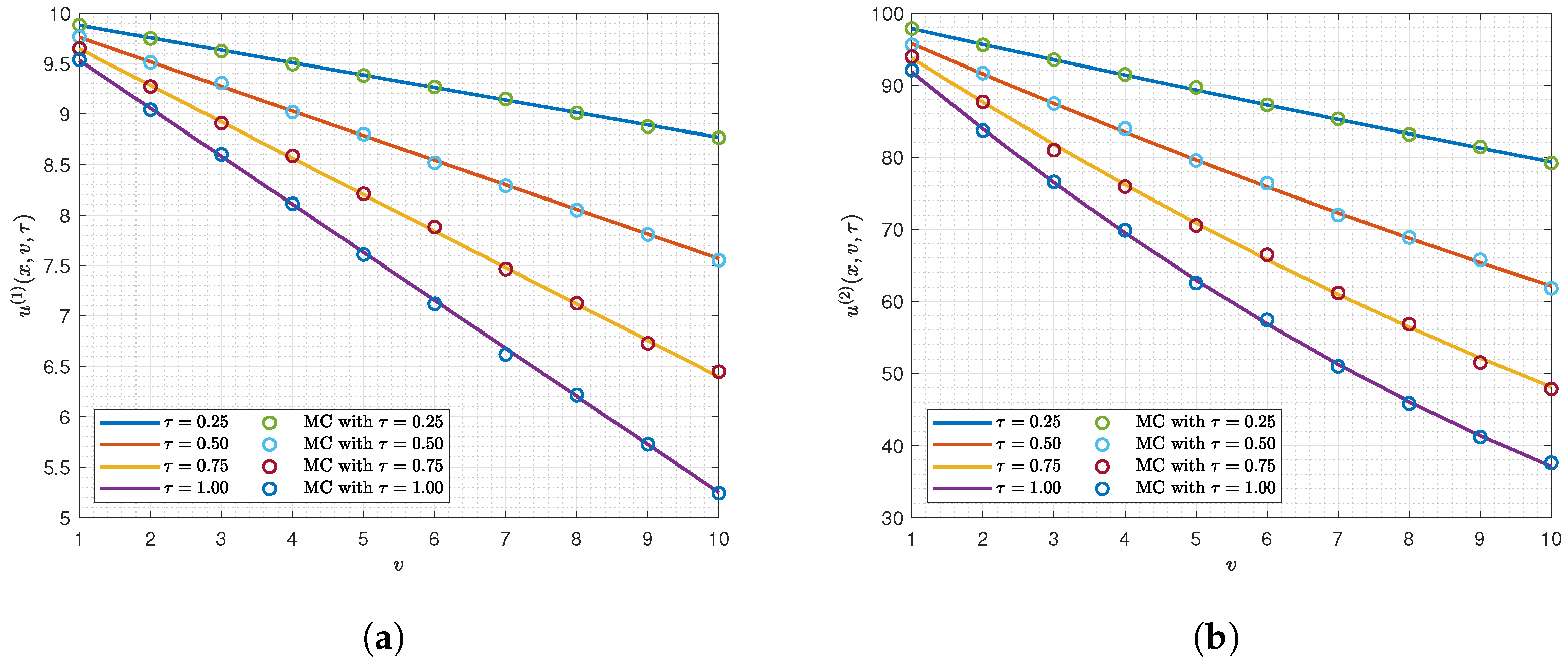
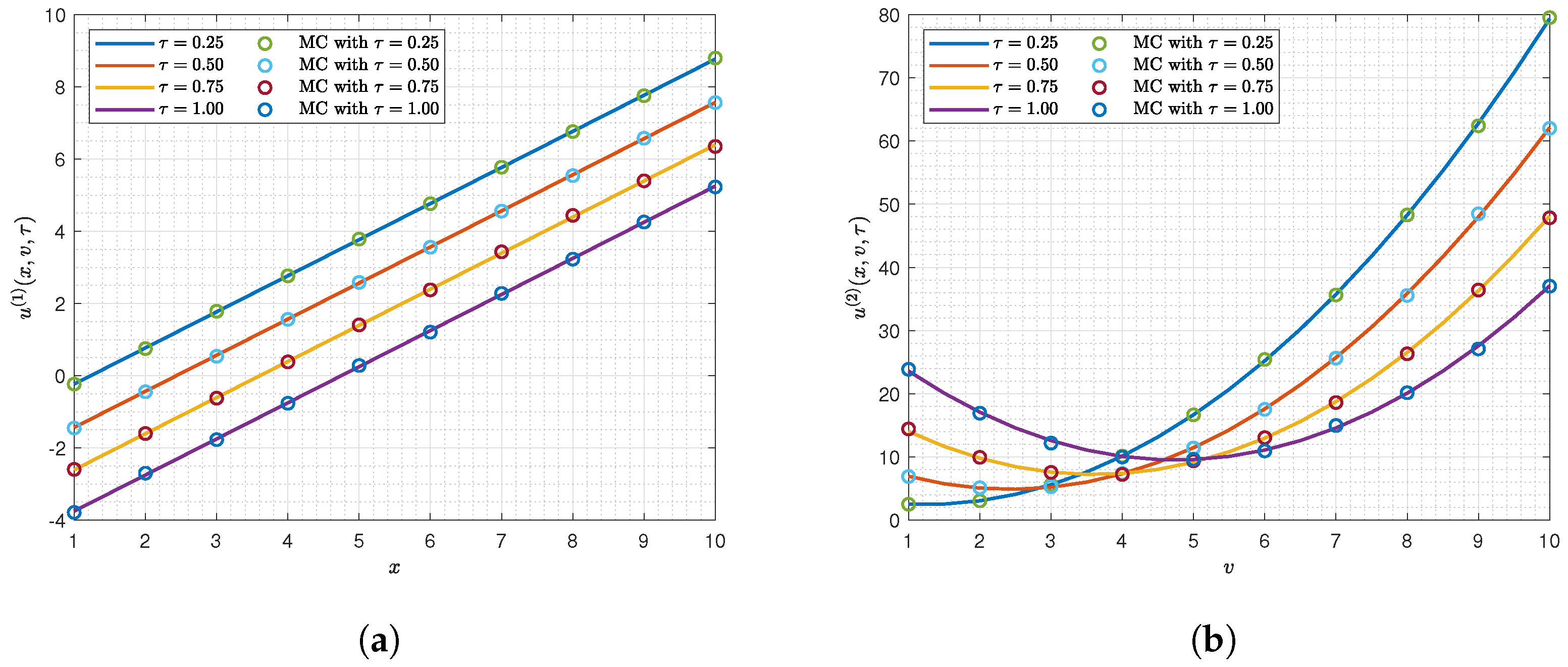
For the numerical testing, we used parameters $r=0.01$, $\kappa =0.1$, $\theta =0.1$, $\rho =0.01$, and $\sigma =0.001$. The comparison results between Formula (7) given in Theorem 1 and the MC simulations with 10,000 sample paths are shown in Figure 2 and Figure 3. These figures illustrate that the results obtained from the MC simulations (colored circles) completely match with the closed-form Formula (7) (colored lines) for the first and second conditional moments, thereby validating the accuracy of the closed-form Formula (7) obtained from Theorem 1.

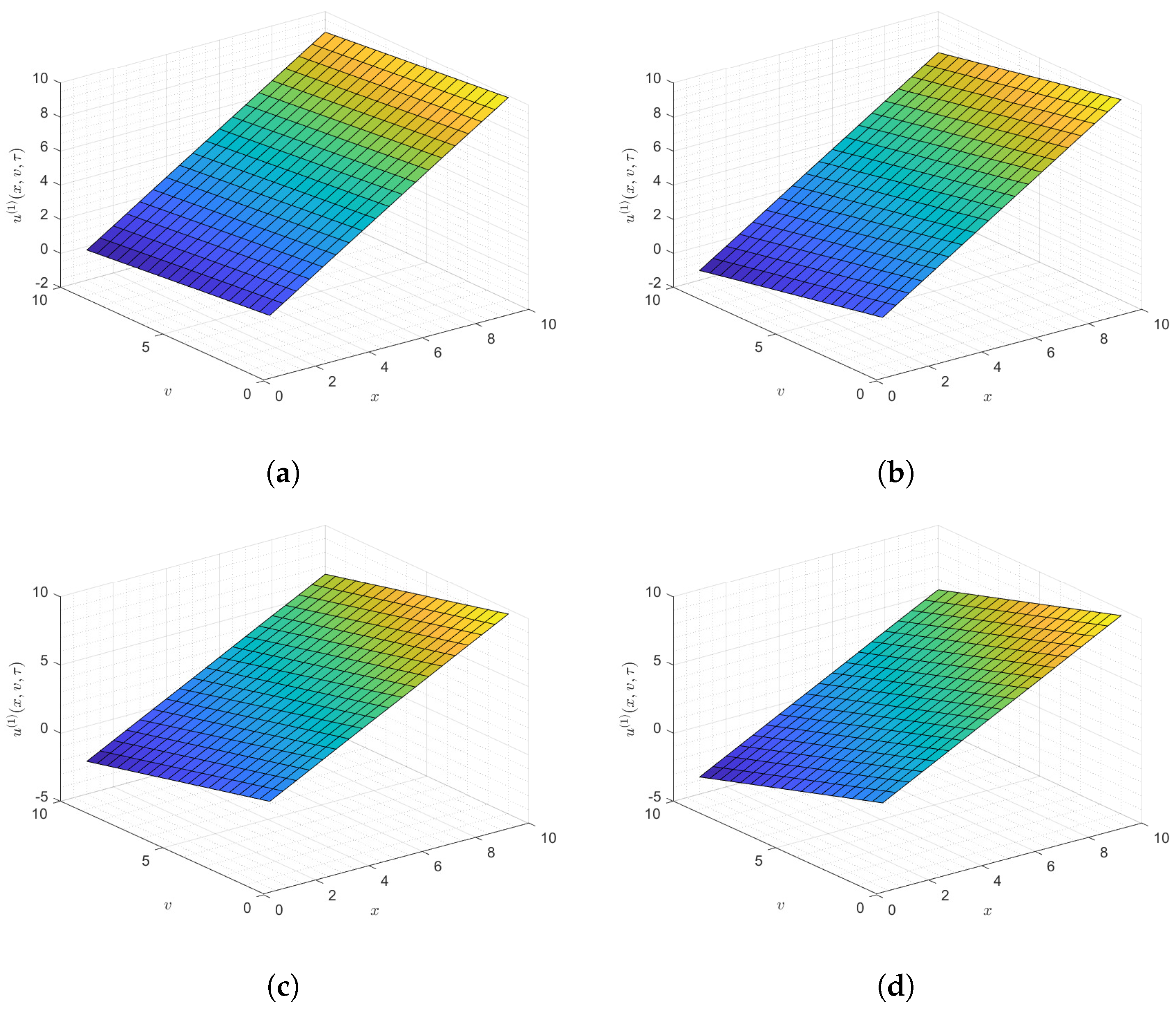
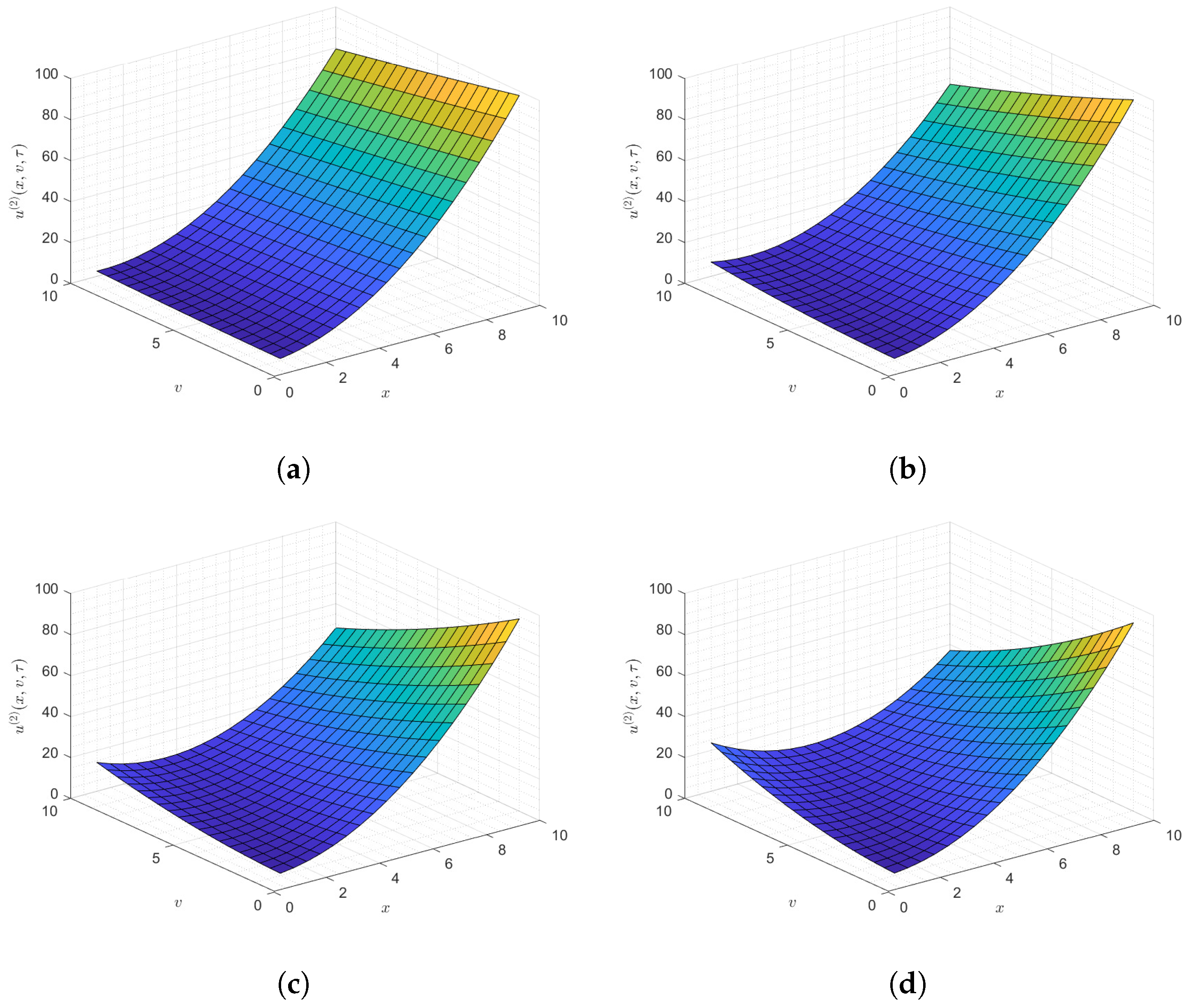
In addition,

Table 1. MAEs of the first conditional moment $u^{\left(1\right)}(x,v,1)$ between our formula and the MC simulations together with the average runtimes of the MC simulations.

x	No. of Paths	$\mathit{v}=1$		$\mathit{v}=5$		$\mathit{v}=10$
		MAEs	ARTs	MAEs	ARTs	MAEs	ARTs
1	20,000	$6.64\times {10}^{-2}$	9.14	$6.80\times {10}^{-2}$	8.78	$6.88\times {10}^{-2}$	10.05
	40,000	$5.43\times {10}^{-2}$	17.98	$6.65\times {10}^{-3}$	19.11	$5.53\times {10}^{-2}$	18.65
	80,000	$3.23\times {10}^{-3}$	36.57	$4.74\times {10}^{-3}$	36.88	$7.51\times {10}^{-3}$	35.52
5	20,000	$6.73\times {10}^{-2}$	8.81	$6.68\times {10}^{-2}$	9.24	$6.14\times {10}^{-2}$	9.11
	40,000	$5.45\times {10}^{-2}$	19.22	$6.28\times {10}^{-3}$	18.05	$5.45\times {10}^{-2}$	18.63
	80,000	$6.54\times {10}^{-3}$	35.64	$4.95\times {10}^{-3}$	37.06	$2.99\times {10}^{-3}$	37.69
10	20,000	$6.72\times {10}^{-2}$	9.54	$7.33\times {10}^{-2}$	9.47	$5.14\times {10}^{-2}$	9.17
	40,000	$5.41\times {10}^{-2}$	18.87	$6.23\times {10}^{-2}$	18.55	$4.45\times {10}^{-2}$	17.57
	80,000	$6.04\times {10}^{-3}$	37.87	$9.55\times {10}^{-3}$	36.14	$8.53\times {10}^{-3}$	36.36

and

Table 2. MAEs of the second conditional moment $u^{\left(2\right)}(x,v,1)$ between our formula and the MC simulations together with the average runtimes of the MC simulations.

x	No. of Paths	$\mathit{v}=1$		$\mathit{v}=5$		$\mathit{v}=10$
		MAEs	ARTs	MAEs	ARTs	MAEs	ARTs
1	20,000	$7.54\times {10}^{-2}$	11.14	$4.15\times {10}^{-2}$	9.54	$6.23\times {10}^{-2}$	10.13
	40,000	$6.87\times {10}^{-3}$	18.05	$7.11\times {10}^{-2}$	19.91	$6.38\times {10}^{-2}$	20.57
	80,000	$4.13\times {10}^{-3}$	39.78	$5.09\times {10}^{-3}$	40.24	$7.99\times {10}^{-3}$	39.76
5	20,000	$5.34\times {10}^{-2}$	10.81	$6.80\times {10}^{-2}$	10.49	$5.41\times {10}^{-2}$	9.61
	40,000	$4.55\times {10}^{-2}$	19.52	$5.69\times {10}^{-3}$	21.59	$3.74\times {10}^{-2}$	21.03
	80,000	$8.54\times {10}^{-3}$	38.30	$2.12\times {10}^{-3}$	39.14	$8.36\times {10}^{-3}$	40.11
10	20,000	$1.25\times {10}^{-2}$	9.98	$7.23\times {10}^{-2}$	10.08	$7.91\times {10}^{-2}$	11.79
	40,000	$7.28\times {10}^{-3}$	20.17	$4.15\times {10}^{-2}$	21.11	$5.11\times {10}^{-2}$	20.50
	80,000	$5.10\times {10}^{-3}$	39.88	$8.83\times {10}^{-2}$	40.47	$8.94\times {10}^{-3}$	39.96

demonstrate the mean absolute errors (MAEs) between Formula (7) and the MC simulations and the average runtimes (ARTs) of the MC simulations for different numbers of the sample paths: 20,000, 40,000, and 80,000, to validate the accuracy and efficiency of our proposed formula. These ARTs are the average of the computational times to calculate the MC simulations for fixing $\tau =1$ at each initial value $x=1,5,10$ and $v=1,5,10$. Table 1 and Table 2 conclude that the more the sample path numbers increase, the more the MAEs decrease. However, the ARTs also increase. Moreover, we can see the efficiency of our proposed Formula (7) from Theorem 1, which provides the exact value of $u^{\left(1\right)}(x,v,\tau )$. Our proposed Formula (7) employs a small computational time around 0.1532 s. Finally, we depict the surface plots of the first and second conditional moments $u^{\left(1\right)}(x,v,\tau )$ and $u^{\left(2\right)}(x,v,\tau )$ by varying $x,v\in [1,10]$ at different $\tau =0.25,0.5,0.75,1$ in Figure 4 and Figure 5.

6. Conclusions

In this study, we derived a closed-form formula of conditional moments for the inhomogeneous Heston model (4) in the term of a polynomial expansion, as provided in Theorem 1. We further presented a formula for the first conditional moment $u^{\left(1\right)}(x,v,\tau )$ proposed in Corollary 1 as a consequence of Theorem 1. Additionally, some essential properties of the inhomogeneous Heston model (4), such as the first and second conditional moments, and the skewness were observed and discussed in Section 4. The algorithm to solve the recursive coefficient functions (8)–(12) given in Theorem 1 was provided in Algorithm 1.

Finally, we validated our closed-form formula for the first and second conditional moments by comparing it with the MC simulations via several experimental examples in Section 5. The experiments in each example indicated that our proposed formula and the MC simulations completely matched. Figure 2 and Figure 3 and Table 1 and Table 2 confirmed that our closed-form formula provides good accuracy and reduces the computational burden compared with the MC simulations.

This technique presented here can be also applied to the other two-factor models, such as Schwartz’s two- or three-factor model. However, one primary concern for our presented formulas is that the coefficients $A_{j,\ell }^{\left(n\right)}\left(\tau \right)$ in (7) cannot be obtained directly by solving the system of recursive ODEs. In such a case, a numerical method is required to manipulate those coefficients.

References

1. Heston, S.L. A closed-form solution for options with stochastic volatility with applications to bond and currency options. Rev. Financ. Stud. 1993, 6, 327–343. [Google Scholar] [CrossRef] [Green Version]
2. Cox, J.C.; Ingersoll, J.E., Jr.; Ross, S.A. A theory of the term structure of interest rates. In Theory of Valuation; World Scientific: Singapore, 2005; pp. 129–164. [Google Scholar]
3. He, X.J.; Zhu, P.S. An alternative form used to calibrate the Heston option pricing model. Comput. Math. Appl. 2016, 71, 1831–1842. [Google Scholar] [CrossRef] [Green Version]
4. He, X.J.; Zhu, P.S. A closed-form pricing formula for European options under the Heston model with stochastic interest rate. J. Comput. Appl. Math. 2018, 335, 323–333. [Google Scholar] [CrossRef] [Green Version]
5. Zeng, X.C.; Zhu, P.S. A new simple tree approach for the Heston’s stochastic volatility model. Comput. Math. Appl. 2019, 78, 1993–2010. [Google Scholar] [CrossRef]
6. Lu, X.; Zhu, P.S.; Yan, D. Nonlinear PDE model for European options with transaction costs under Heston stochastic volatility. Commun. Nonlinear Sci. Numer. Simul. 2021, 103, 105986. [Google Scholar] [CrossRef]
7. Zhu, P.S.; Lian, G.H. On the convexity correction approximation in pricing volatility swaps and VIX futures. New Math. Natural Comput. 2018, 14, 383–401. [Google Scholar] [CrossRef]
8. He, X.J.; Zhu, P.S. A series-form solution for pricing variance and volatility swaps with stochastic volatility and stochastic interest rate. Comput. Math. Appl. 2018, 76, 2223–2234. [Google Scholar] [CrossRef]
9. Zhu, P.S.; Lian, G.H. A closed-form exact solution for pricing variance swaps with stochastic volatility. Math. Financ. Int. J. Math. Stat. Financ. Econ. 2011, 21, 233–256. [Google Scholar]
10. Zhu, P.S.; Lian, G.H. On the valuation of variance swaps with stochastic volatility. Appl. Math. Comput. 2012, 219, 1654–1669. [Google Scholar] [CrossRef]
11. Zhu, P.S.; Lian, G.H. Analytically pricing volatility swaps under stochastic volatility. J. Comput. Appl. Math. 2015, 288, 332–340. [Google Scholar] [CrossRef]
12. Batrancea, L. An econometric approach regarding the impact of fiscal pressure on equilibrium: Evidence from electricity, gas and oil companies listed on the New York Stock Exchange. Mathematics 2021, 9, 630. [Google Scholar] [CrossRef]
13. Batrancea, L.; Rus, M.I.; Masca, E.S.; Morar, I.D. Fiscal Pressure as a Trigger of Financial Performance for the Energy Industry: An Empirical Investigation across a 16-Year Period. Energies 2021, 14, 3769. [Google Scholar] [CrossRef]
14. Batrancea, L.; Rathnaswamy, M.K.; Batrancea, I. A panel data analysis on determinants of economic growth in seven non-BCBS Countries. J. Knowl. Econ. 2021, 12, 1–15. [Google Scholar] [CrossRef]
15. Hansen, L.P.; Scheinkman, J.A. Back to the Future: Generating Moment Implications for Continuous-Time Markov Processes. Econometrica 1995, 63, 767–804. [Google Scholar] [CrossRef]
16. Hull, J.; White, A. Pricing interest-rate-derivative securities. Rev. Financ. Stud. 1990, 3, 573–592. [Google Scholar] [CrossRef]
17. Maghsoodi, Y. Solution of the extended CIR term structure and bond option valuation. Math. Financ. 1996, 6, 89–109. [Google Scholar] [CrossRef]
18. Rujivan, S. A closed-form formula for the conditional moments of the extended CIR process. J. Comput. Appl. Math. 2016, 297, 75–84. [Google Scholar] [CrossRef]
19. Nonsoong, P.; Mekchay, K.; Rujivan, S. An analytical option pricing formula for mean-reverting asset with time-dependent parameter. ANZIAM J. 2021, 63, 178–202. [Google Scholar]
20. Grzelak, L.A.; Oosterlee, C.W. On the Heston model with stochastic interest rates. SIAM J. Financ. Math. 2011, 2, 255–286. [Google Scholar] [CrossRef] [Green Version]
21. Karatzas, I.; Shreve, S. Brownian Motion and Stochastic Calculus; Springer Science & Business Media: New York, NY, USA, 2012; Volume 113. [Google Scholar]
22. Strang, G. Introduction to Linear Algebra; Wellesley-Cambridge Press: Wellesley, MA, USA, 1993; Volume 3. [Google Scholar]
23. Rogers, L.C.G.; Williams, D. Diffusions, Markov Processes and Martingales: Volume 2, Itô Calculus; Cambridge University Press: Cambridge, UK, 2000; Volume 2. [Google Scholar]
24. Ekström, E.; Lötstedt, P.; Tysk, J. Boundary values and finite difference methods for the single factor term structure equation. Appl. Math. Financ. 2009, 16, 253–259. [Google Scholar] [CrossRef]
25. Forman, J.L.; Sørensen, M. The Pearson diffusions: A class of statistically tractable diffusion processes. Scand. J. Stat. 2008, 35, 438–465. [Google Scholar] [CrossRef]
26. Schmidt, M.F. Pearson Diffusions with Jumps. Ph.D. Thesis, Technische Universitat Munchen, München, Germany, 2008. [Google Scholar]
27. Sutthimat, P.; Mekchay, K.; Rujivan, S. Explicit formula for conditional expectations of product of polynomial and exponential function of affine transform of extended Cox-Ingersoll-Ross process. J. Phys. Conf. Ser. IOP Pub. 2018, 1132, 012083. [Google Scholar] [CrossRef]
28. Sutthimat, P.; Rujivan, S.; Mekchay, K.; Rakwongwan, U. Analytical formula for conditional expectations of path-dependent product of polynomial and exponential functions of extended Cox–Ingersoll–Ross process. Res. Math. Sci. 2022, 9, 1–17. [Google Scholar] [CrossRef]
29. Sutthimat, P.; Mekchay, K. Closed-form formulas for conditional moments of inhomogeneous Pearson diffusion processes. Commun. Nonlinear Sci. Numer. Simul. 2022, 106, 106095. [Google Scholar] [CrossRef]
30. Chumpong, K.; Mekchay, K.; Rujivan, S. A simple closed-form formula for the conditional moments of the Ornstein–Uhlenbeck process. Songklanakarin J. Sci. Technol. 2020, 42, 836–845. [Google Scholar]
31. Chumpong, K.; Mekchay, K.; Thamrongrat, N. Analytical formulas for pricing discretely-sampled skewness and kurtosis swaps based on Schwartz’s one-factor model. Songklanakarin J. Sci. Technol. 2021, 43, 1–6. [Google Scholar]
32. Rujivan, S.; Zhu, P.S. A simplified analytical approach for pricing discretely-sampled variance swaps with stochastic volatility. Appl. Math. Lett. 2012, 25, 1644–1650. [Google Scholar] [CrossRef] [Green Version]
33. Han, Y.; Zhao, L. A closed-form pricing formula for variance swaps under MRG–Vasicek model. Comput. Appl. Math. 2019, 38, 1–17. [Google Scholar] [CrossRef]
34. Zheng, W.; Kwok, Y.K. Closed form pricing formulas for discretely sampled generalized variance swaps. Math. Financ. 2014, 24, 855–881. [Google Scholar] [CrossRef]
35. Boonklurb, R.; Duangpan, A.; Treeyaprasert, T. Modified finite integration method using Chebyshev polynomial for solving linear differential equations. J. Numer. Ind. Appl. Math 2018, 12, 1–19. [Google Scholar]
36. Boonklurb, R.; Duangpan, A.; Gugaew, P. Numerical solution of direct and inverse problems for time-dependent Volterra integro-differential equation using finite integration method with shifted Chebyshev polynomials. Symmetry 2020, 12, 497. [Google Scholar] [CrossRef] [Green Version]
37. Duangpan, A.; Boonklurb, R.; Juytai, M. Numerical solutions for systems of fractional and classical integro-differential equations via Finite Integration Method based on shifted Chebyshev polynomials. Fractal Fract. 2021, 5, 103. [Google Scholar] [CrossRef]
38. Oosterlee, C.W.; Grzelak, L.A. Mathematical Modeling and Computation in Finance: With Exercises and Python and Matlab Computer Codes; World Scientific: Singapore, 2019. [Google Scholar]
39. Asmussen, S.; Glynn, P.W. Stochastic Simulation: Algorithms and Analysis; Springer Science & Business Media: New York, NY, USA, 2007; Volume 57. [Google Scholar]
Figure 1. Diagram for solving recursive coefficient functions from A n , n ( n ) to A 0 , 0 ( n ) .
Computation 10 00046 g001
Figure 2. Validation tests of the first and second conditional moments for the initial values x = 10 and v = 1 , 2 , 3 , , 10 at different τ = 0.25 , 0.5 , 0.75 , 1 . (a) The first conditional moment u ( 1 ) ( 10 , v , τ ) . (b) The second conditional moment u ( 2 ) ( 10 , v , τ ) .
Computation 10 00046 g002
Figure 3. Validation tests of the first and second conditional moments for the initial values v = 10 and x = 1 , 2 , 3 , , 10 at different τ = 0.25 , 0.5 , 0.75 , 1 . (a) The first conditional moment u ( 1 ) ( x , 10 , τ ) . (b) The second conditional moment u ( 2 ) ( x , 10 , τ ) .
Computation 10 00046 g003
Figure 4. Surface plots of the first conditional moment u ( 1 ) ( x , v , τ ) by varying x , v [ 1 , 10 ] at different values of τ . (a) u ( 1 ) ( x , v , 0.25 ) . (b) u ( 1 ) ( x , v , 0.5 ) . (c) u ( 1 ) ( x , v , 0.75 ) . (d) u ( 1 ) ( x , v , 1 ) .
Computation 10 00046 g004
Figure 5. Surface plots of the second conditional moment u ( 2 ) ( x , v , τ ) by varying x , v [ 1 , 10 ] at different values of τ . (a) u ( 2 ) ( x , v , 0.25 ) . (b) u ( 2 ) ( x , v , 0.5 ) . (c) u ( 2 ) ( x , v , 0.75 ) . (d) u ( 2 ) ( x , v , 1 ) .
Computation 10 00046 g005