Hierarchical Epidemic Model on Structured Population: Diffusion Patterns and Control Policies


Abstract
:1. Introduction
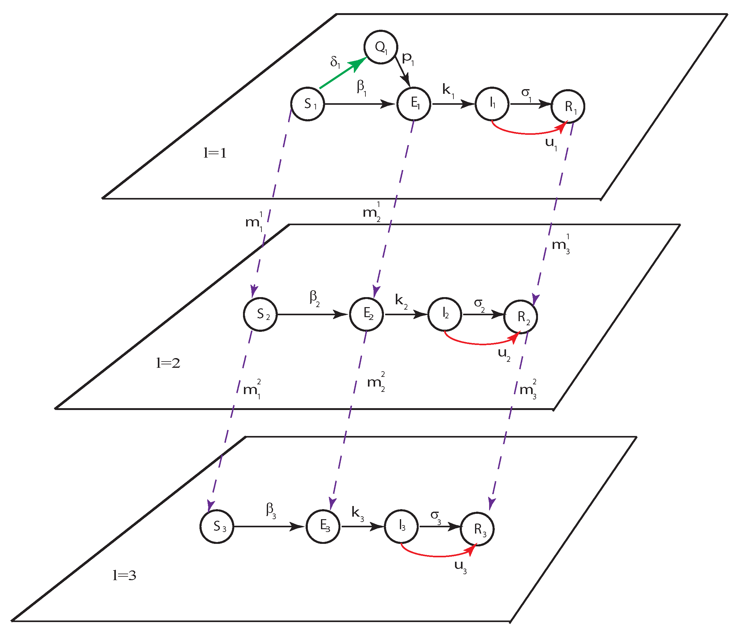
2. Deterministic Epidemic Model
- , , , ,
- , ,
- , .
3. Basic Reproduction Number
4. Optimal Control Problem
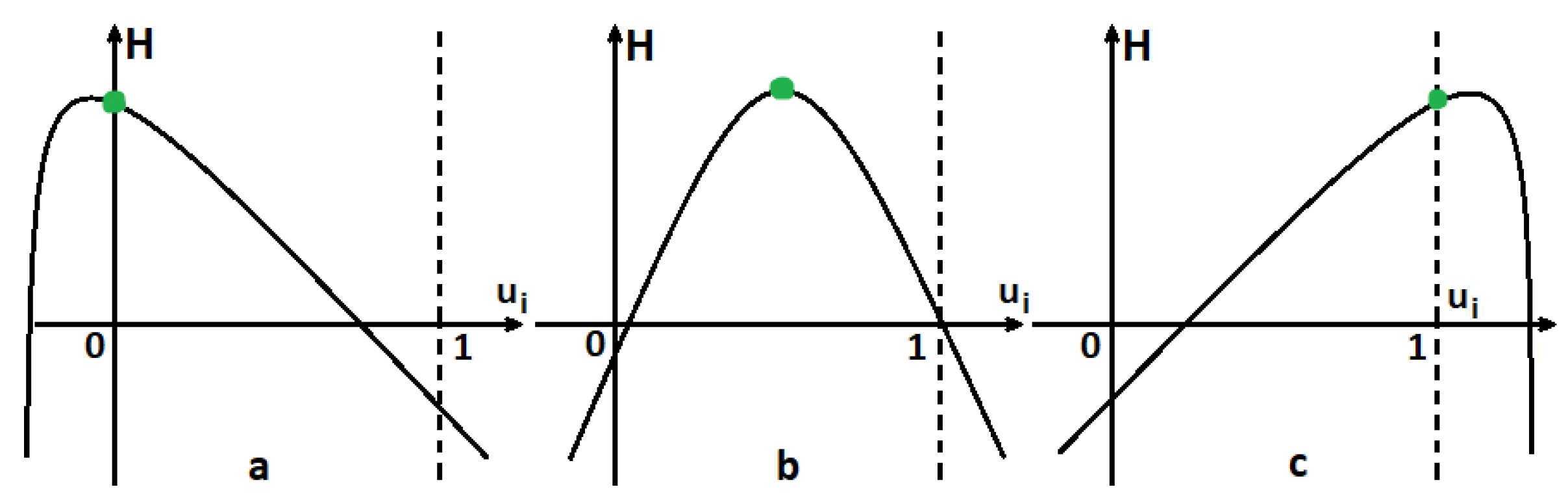
4.1. Functions Are Concave
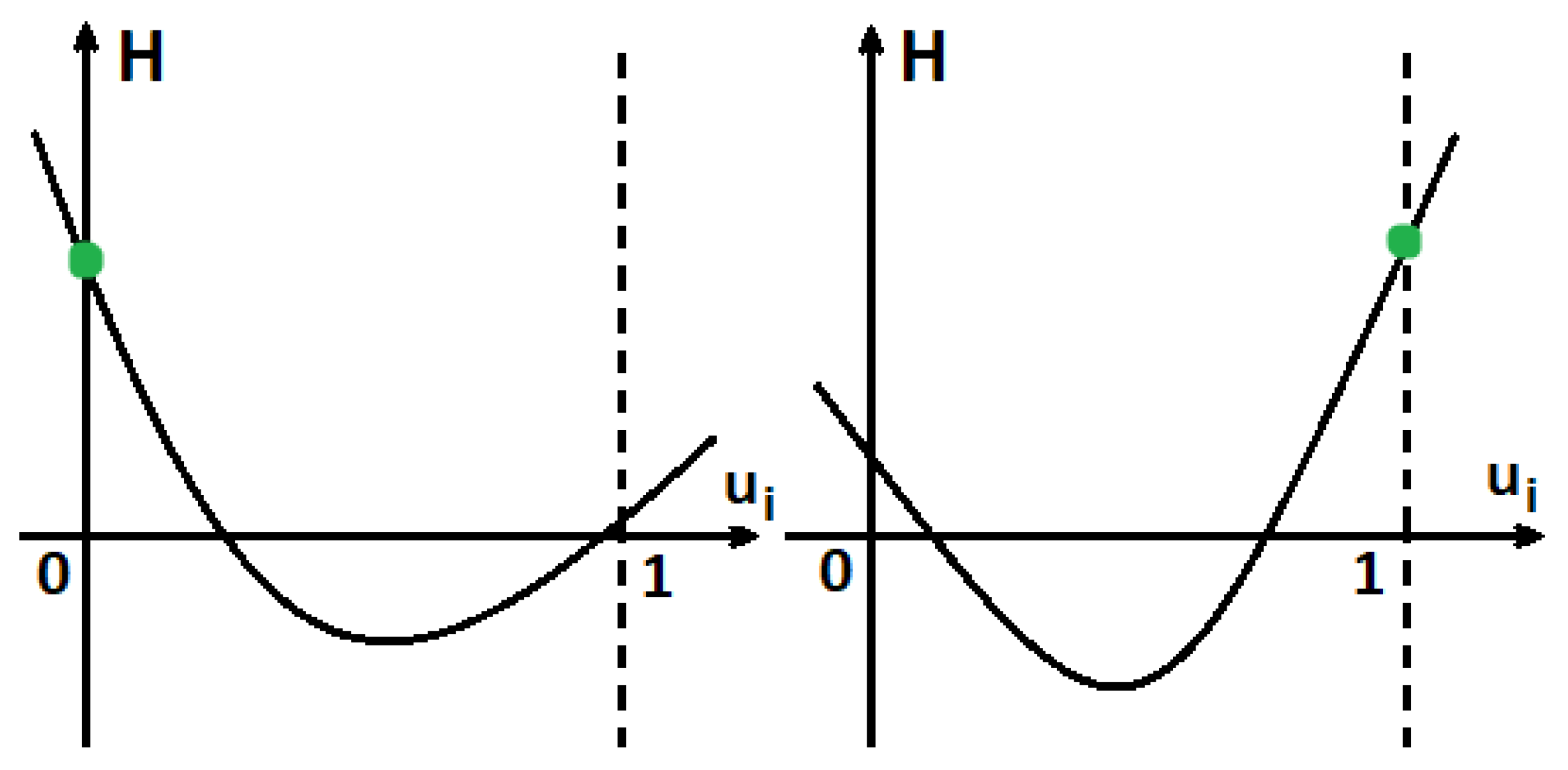
4.2. Functions Are Strictly Convex
5. Numerical Simulation
6. Conclusions
Author Contributions
Funding
Institutional Review Board Statement
Informed Consent Statement
Data Availability Statement
Conflicts of Interest
Appendix A
References
- Jones, C.J.; Philippon, T.; Venkateswaran, V. Optimal Mitigation Policies in a Pandemic: Social Distancing and Working from Home; Working Paper 26984; National Bureau of Economic Research: Cambridge, MA, USA, 2020. [Google Scholar]
- Masuda, N.; Konno, N. Multi-state epidemic processes on complex networks. J. Theor. Biol. 2006, 243, 64–75. [Google Scholar] [CrossRef] [Green Version]
- Nuno, M.; Feng, Z.; Martcheva, M.; Castillo-Chavez, C. Dynamics of two-strain influenza with isolation and partial cross-immunity. SIAM J. Appl. Math. 2005, 65, 964–982. [Google Scholar] [CrossRef] [Green Version]
- Smith, G.J.; Vijaykrishna, D.; Bahl, J.; Lycett, S.J.; Worobey, M.; Pybus, O.G.; Ma, S.K.; Cheung, C.L.; Raghwani, J.; Bhatt, S.; et al. Origins and evolutionary genomics of the 2009 swine-origin H1N1 influenza A epidemic. Nature 2009, 459, 1122–1125. [Google Scholar] [CrossRef] [PubMed] [Green Version]
- Butler, D. Flu surveillance lacking. Nature 2012, 483, 520–522. [Google Scholar] [CrossRef] [Green Version]
- Moon, A.S.; Sahneh, F.D.; Scoglio, C. Generalized group-based epidemic model for spreading processes on networks: GgroupEM. arXiv 2019, arXiv:1908.06057. [Google Scholar]
- Sahneh, F.D.; Scoglio, C.; Mieghem, P.V. Generalized epidemic meanfield model for spreading processes over multilayer complex networks. IEEE/ACM Trans. Netw. 2013, 21, 1609–1620. [Google Scholar] [CrossRef]
- Vespignani, A.; Pastor-Satorras, R.; Van Mieghem, M.; Castellano, C. Epidemic processes in complex networks. Rev. Mod. Phys. 2015, 87, 925. [Google Scholar]
- Evans, A.S.; Kaslow, R.A. Viral Infections of Humans: Epidemiology and Control; Springer: New York, NY, USA, 1997. [Google Scholar]
- Fedyanin, D.N.; Chkhartishvili, A.G. On a model of informational control in social networks. Autom. Remote Control 2011, 72, 2181–2187. [Google Scholar] [CrossRef]
- Khan, M.A.; Shah, S.W.; Ullah, S.; Gómez-Aguilar, J.F. A dynamical model of asymptomatic carrier zika virus with optimal control strategies. Nonlinear Anal. Real World Appl. 2019, 50, 144–170. [Google Scholar] [CrossRef]
- Sharma, S.; Samanta, G.P. Stability analysis and optimal control of an epidemic model with vaccination. Int. J. Biomath. 2015, 8, 28. [Google Scholar] [CrossRef]
- Taynitskiy, V.A.; Gubar, E.A.; Zhitkova, E.M. Structure of optimal control in the model of propagation of two malicious softwares. In Proceedings of the International Conference on Stability and Control Processes in Memory of V.I. Zubov (SCP), St. Petersburg, Russia, 5–9 October 2015; pp. 261–264. [Google Scholar]
- Taynitskiy, V.A.; Gubar, E.A.; Zhu, Q. Optimal Security Policy for Protection Against Heterogeneous Malware. In International Conference on Network Games, Control and Optimization (NETGCOOP 2016); Birkhäuser: Cham, Switzerland, 2017. [Google Scholar]
- Wu, Q.; Small, M.; Liu, H. Superinfection Behaviors on Scale-Free Networks with Competing Strains. J. Nonlinear Sci. 2013, 23, 113–127. [Google Scholar] [CrossRef]
- Zuzek, L.G.A.; Stanley, H.E.; Braunstein, L.A. Epidemic Model with Isolation in Multilayer Networks. Sci. Rep. 2015, 5, 12151. [Google Scholar] [CrossRef] [PubMed] [Green Version]
- Funk, S.; Gilad, E.; Watkins, C.; Jansen, V.A.A. The spread of awareness and its impact on epidemic outbreaks. Proc. Natl. Acad. Sci. USA 2009, 106, 6872–6877. [Google Scholar] [CrossRef] [PubMed] [Green Version]
- Nekovee, A.M.; Moreno, Y.; Bianconi, G.; Marsili, M. Theory of rumor spreading in complex social networks. Physica 2007, A374, 457–470. [Google Scholar]
- Newman, L.H. What We Know about Fridayś Massive East Coast Internet Outage. Wired Magazine. 24 October 2016. Available online: https://www.wired.com/2016/10/internet-outage-ddos-dns-dyn/ (accessed on 21 October 2016).
- Merler, S.; Ajelli, M.; Fumanelli, L.; Gomes, M.F.; y Piontti, A.P.; Rossi, L.; Chao, D.L.; Longini, I.M., Jr.; Halloran, M.E.; Vespignani, A. Spatiotemporal spread of the 2014 outbreak of Ebola virus disease in Liberia and the effectiveness of non-pharmaceutical interventions: A computational modelling analysis. Lancet Infect. Dis. 2015, 15, 204–211. [Google Scholar] [CrossRef] [Green Version]
- Nowzari, C.; Preciado, V.M.; Pappas, G.J. Analysis and Control of Epidemics: A Survey of Spreading Processes on Complex Networks. IEEE Control Syst. Mag. 2016, 36, 26–46. [Google Scholar]
- Altman, E.; Avrachenkov, K.; De Pellegrini, F.; El-Azouzi, R.; Wang, H. Multilevel Strategic Interaction Game Models for Complex Networks; Springer Nature: Cham, Switzerland, 2019. [Google Scholar]
- Taynitskiy, V.; Gubar, E.; Fedyanin, D.; Petrov, I.; Zhu, Q. Optimal Control of Joint Multi-Virus Infection and Information Spreading. IFAC-PapersOnLine 2020, 53, 6650–6655. [Google Scholar] [CrossRef]
- Huang, Y.; Zhu, Q. A differential game approach to decentralized virus-resistant weight adaptation policy over complex networks. IEEE Trans. Control Netw. Syst. 2019, 7, 944–955. [Google Scholar] [CrossRef] [Green Version]
- Fenichel, E. Economic considerations for social distancing and behavioural-based policies during an epidemic. J. Health Econ. 2013, 32, 440–451. [Google Scholar] [CrossRef] [Green Version]
- Geoffard, P.Y.; Philipson, T. Rational Epidemics and Their Public Control. Int. Econ. Rev. 1996, 37, 603–624. [Google Scholar] [CrossRef]
- Alvarez, F.; Argente, D.; Lippi, F. A Simple Planning Problem for COVID-19 Lockdown; Working Paper 26981; National Bureau of Economic Research: Cambridge, MA, USA, 2020. [Google Scholar]
- Eichenbaum, M.; Rebelo, S.; Trabandt, M. The Macroeconomics of Epidemics; Working Paper 26882; National Bureau of Economic Research: Cambridge, MA, USA, 2020. [Google Scholar]
- Farboodi, M.; Jarosch, G.; Shimer, R. Internal and External Effects of Social Distancing in a Pandemic; Working Paper 27059; National Bureau of Economic Research: Cambridge, MA, USA, 2020. [Google Scholar]
- Garriga, C.; Manuelli, R.; Sanghi, S. Optimal Management of an Epidemic: An Application to COVID-19; A Progress Report; Mimeo: New York, NY, USA, 2020. [Google Scholar]
- Piguillem, F.; Shi, L. Optimal Covid-19 Quarantine and Testing Policies. CEPR Discussion Paper No. DP14613. 2020. Available online: https://ssrn.com/abstract=3594243 (accessed on 8 May 2020).
- Rowthorn, R.; Flavio, T. The Optimal Control of Infectious Diseases Via Prevention and Treatment; Technical Report 2013, Cambridge-INET Working Paper; Faculty of Economics, University of Cambridge: Cambridge, UK, 2020. [Google Scholar]
- Acemoglu, D.; Chernozhukov, V.; Werning, I.; Winston, M.D. Optimal Targeted Lockdowns in a MultiGroup SIR Model. Am. Econ. Rev. Insights 2021, 3, 487–502. [Google Scholar] [CrossRef]
- Bailey, N.T.J. The Mathematical Theory of Infectious Diseases, 2nd ed.; Hafner: New York, NY, USA, 1975. [Google Scholar]
- Hethcote, H.W.; Van Ark, J.W. Epidemiological models for heterogeneous populations: Proportionate mixing, parameter estimation, and immunization programs. Math. Biosci. 1987, 84, 85–118. [Google Scholar] [CrossRef]
- Eshghi, S.; Khouzani, M.H.R.; Sarkar, S.; Venkatesh, S.S. Optimal patching in clustered malware epidemics. IEEE/ACM Trans. Netw. 2014, 24, 283–298. [Google Scholar] [CrossRef] [Green Version]
- Ndeffo Mbah, M.L.; Gilligan, C.A. Resource allocation for epidemic control in metapopulations. PLoS ONE 2011, 6, e24577. [Google Scholar] [CrossRef]
- Rowthorn, R.E.; Laxminarayan, R.; Gilligan, C.A. Optimal control of epidemics in metapopulations. J. R. Soc. Interface 2009, 6, 1135–1144. [Google Scholar] [CrossRef] [Green Version]
- Holloway, R.; Rasmussen, S.A.; Zaza, S.; Cox, N.J.; Jernigan, D.B. Influenza Pandemic Framework Workgroup. Updated preparedness and response framework for influenza pandemics. Morb. Mortal. Wkly. Rep. Recomm. Rep. 2014, 63, 1–18. [Google Scholar]
- Lauer, S.A.; Grantz, K.H.; Bi, Q.; Jones, F.K.; Zheng, Q.; Meredith, H.R.; Azman, A.S.; Reich, N.G.; Lessler, J. The Incubation Period of Coronavirus Disease 2019 (COVID-19) from Publicly Reported Confirmed Cases: Estimation and Application. Available online: https://www.acpjournals.org/doi/10.7326/M20-0504 (accessed on 10 March 2020).
- Nishiura, H.; Kobayashi, T.; Miyama, T.; Suzuki, A.; Jung, S.M.; Hayashi, K.; Kinoshita, R.; Yang, Y.; Yuan, B.; Akhmetzhanov, A.R.; et al. Estimation of the asymptomatic ratio of novel coronavirus infections (COVID-19). Int. J. Infect. Dis. 2020, 94, 154–155. [Google Scholar] [CrossRef] [PubMed]
- Poletti, P.; Tirani, M.; Cereda, D.; Trentini, F.; Guzzetta, G.; Sabatino, G.; Marziano, V.; Castrofino, C.; Grosso, F.; Castillo, G.; et al. Association of Age with Likelihood of Developing Symptoms and Critical Disease among Close Contacts Exposed to Patients with Confirmed SARS-CoV-2 Infection in Italy. Available online: https://jamanetwork.com/journals/jamanetworkopen/fullarticle/2777314 (accessed on 10 March 2020).
- Allen, L.J.S. An introduction to stochastic epidemic models. In Mathematical Epidemiology; Springer: Berlin/Heidelberg, Germany, 2008; pp. 81–130. [Google Scholar]
- Capasso, V. Mathematical Structures of Epidemic Systems; Springer: Berlin/Heidelberg, Germany, 1993; Volume 97. [Google Scholar]
- Diekmann, O.; Heesterbeek, A.P.; Roberts, M.G. The construction of next-generation matrices for compartmental epidemic models. J. R. Soc. Interface 2010, 7, 873–885. [Google Scholar] [CrossRef] [PubMed] [Green Version]
- Van den Driessche, P. Reproduction numbers of infectious disease models. Infect. Dis. Model. 2017, 2, 288–303. [Google Scholar] [CrossRef]
- Jones, J.H. Notes on R0; Department of Anthropological Sciences: Stanford, CA, USA, 2007; Volume 323, pp. 1–19. [Google Scholar]
- Altman, E.; Khouzani, M.; Sarkar, S. Optimal control of epidemic evolution. In Proceedings of the INFOCOM, Shanghai, China, 10–15 April 2011; pp. 1683–1691. [Google Scholar]
- Fu, F.; Rosenbloom, D.I.; Wang, L.; Nowak, M.A. Imitation dynamics of vaccination behaviour on social networks. Proc. R. Soc. B Biol. Sci. 2011, 278, 42–49. [Google Scholar] [CrossRef] [Green Version]
- Pontryagin, L.; Boltyanskii, V.; Gamkrelidze, R.; Mishchenko, E. The Mathematical Theory of Optimal Processes; Interscience: Moscow, Russia, 1962. [Google Scholar]
- Sethi, S.P.; Thompson, G.L. Optimal Control Theory: Applications to Management Science and Economics; Springer: Berlin, Germany, 2006. [Google Scholar]
- Taynitskiy, V.; Gubar, E.; Zhu, Q. Optimal Control of Heterogeneous Mutating Viruses. Games 2018, 9, 103. [Google Scholar]
- Gubar, E.A.; Taynitskiy, V.A.; Policardo, L.; Carrera, E.J.S. Optimal Lockdown Policies driven by Socioeconomic Costs. arXiv 2021, arXiv:2105.08349. [Google Scholar]


| Parameters Used for Simulations | |||||
|---|---|---|---|---|---|
| Parameter Name | Exp. 1 | Exp. 2 | Exp. 3 | Exp. 4 | Exp. 5 |
| Fraction of | 0.7 | 0.7 | 0.7 | 0.7 | 0.7 |
| susceptible people | 1 | 1 | 1 | 1 | 1 |
| at time () | 1 | 1 | 1 | 1 | 1 |
| Fraction of | 0.1 | 0.1 | 0.1 | 0.1 | 0.1 |
| exposed people | 0 | 0 | 0 | 0 | 0 |
| at time () | 0 | 0 | 0 | 0 | 0 |
| Fraction of | 0.2 | 0.2 | 0.2 | 0.2 | 0.2 |
| infected people | 0 | 0 | 0 | 0 | 0 |
| at time () | 0 | 0 | 0 | 0 | 0 |
| Infection rate | 0.25 | 0.25 | 0.25 | 0.25 | 0.25 |
| from to () | |||||
| Recovery rate () | 0.1 | 0.1 | 0.1 | 0.1 | 0.1 |
| Asymptomatic to | 0.15 | 0.15 | 0.15 | 0.15 | 0.15 |
| Infected () | |||||
| Voluntary | 0 | 0.4 | 0.6 | 0.3 | 0–1 |
| self-isolation () | |||||
| Return from | 0 | 0.05 | 0 | 0.2 | 0–0.5 |
| self-isolation (p) | |||||
| Migration rates | 0.05 | 0.05 | 0.05 | 0.05 | 0–0.3 |
| from to () | |||||
| Migration rates | 0.05 | 0.05 | 0.05 | 0.05 | 0–0.3 |
| from to () | |||||
| Migration rates | 0.05 | 0.05 | 0.05 | 0.05 | 0–0.3 |
| from to () | |||||
| Infection costs | 1 | 1 | 1 | 1 | 1 |
| Treatment costs | 1 | 1 | 1 | 1 | 1 |
| Maximum values | 0.2 | 0.2 | 0.2 | 0.2 | 0.2 |
| of control () | |||||
| Aggregated costs J | 29.41 | 29.43 | 23.57 | 29.58 | − |
| Uncontrolled case | |||||
| Aggregated costs J | 13.22 | 14.07 | 10.60 | 13.52 | |
| Controlled case | |||||
Publisher’s Note: MDPI stays neutral with regard to jurisdictional claims in published maps and institutional affiliations. |
© 2022 by the authors. Licensee MDPI, Basel, Switzerland. This article is an open access article distributed under the terms and conditions of the Creative Commons Attribution (CC BY) license (https://creativecommons.org/licenses/by/4.0/).
Share and Cite
Gubar, E.; Taynitskiy, V.; Fedyanin, D.; Petrov, I. Hierarchical Epidemic Model on Structured Population: Diffusion Patterns and Control Policies. Computation 2022, 10, 31. https://doi.org/10.3390/computation10020031
Gubar E, Taynitskiy V, Fedyanin D, Petrov I. Hierarchical Epidemic Model on Structured Population: Diffusion Patterns and Control Policies. Computation. 2022; 10(2):31. https://doi.org/10.3390/computation10020031
Chicago/Turabian StyleGubar, Elena, Vladislav Taynitskiy, Denis Fedyanin, and Ilya Petrov. 2022. "Hierarchical Epidemic Model on Structured Population: Diffusion Patterns and Control Policies" Computation 10, no. 2: 31. https://doi.org/10.3390/computation10020031
APA StyleGubar, E., Taynitskiy, V., Fedyanin, D., & Petrov, I. (2022). Hierarchical Epidemic Model on Structured Population: Diffusion Patterns and Control Policies. Computation, 10(2), 31. https://doi.org/10.3390/computation10020031