Abstract
We consider kinetic energy functionals that depend, beside the usual semilocal quantities (density, gradient, Laplacian of the density), on a generalized Yukawa potential, that is the screened Coulomb potential of the density raised to some power. These functionals, named Yukawa generalized gradient approximations (yGGA), are potentially efficient real-space semilocal methods that include significant non-local effects and can describe different important exact properties of the kinetic energy. In this work, we focus in particular on the linear response behavior for the homogeneous electron gas (HEG). We show that such functionals are able to reproduce the exact Lindhard function behavior with a very good accuracy, outperforming all other semilocal kinetic functionals. These theoretical advances allow us to perform a detailed analysis of a special class of yGGAs, namely the linear yGGA functionals. Thus, we show how the present approach can generalize the yGGA functionals improving the HEG linear behavior and leading to an extended formula for the kinetic functional. Moreover, testing on several jellium cluster model systems allows highlighting advantages and limitations of the linear yGGA functionals and future perspectives for the development of yGGA kinetic functionals.
1. Introduction
The non-interacting kinetic energy (KE) functional is one of the main quantities of interest in density functional theory [1,2]. Its exact formal definition is readily obtained, following the Levy constrained search formalism [3], as
where n is the electron density and is a Kohn-Sham (KS) [4] Slater determinant yielding the density n. This formula allows us to study different important properties of the KE functional and provides an explicit expression for in terms of KS orbitals. However, it does not allow us to obtain an explicit expression in terms of the electron density. Therefore, the quest for the KE density functional is still open, also considering the importance of this quantity in many contexts including orbital-free density functional theory (OF-DFT) [5,6,7,8], subsystem DFT [9,10,11,12,13,14,15], and quantum hydrodynamic theory [16,17,18,19]. In addition, semilocal KE functionals have been used in meta-GGA exchange-correlation functionals to remove their orbital dependence [20,21,22,23,24].
Numerous investigations have been dedicated in the last decades to the study of KE functionals [25,26,27,28,29,30,31,32,33,34,35,36,37,38,39,40,41,42,43,44,45,46,47,48,49,50,51,52,53,54,55,56,57,58,59,60,61,62,63,64,65,66,67,68,69,70,71,72]. Nevertheless, accurate approximations of are hard to obtain because this quantity usually gives a dominant contribution to the ground-state energy [3] and because of the highly non-local nature of the KE functional [5,51,73,74,75,76,77,78]. For this reason, more recently, machine-learning methods have also been used to develop KE functionals [79,80,81,82,83,84,85,86,87].
A KE functional approximation can be written
where is the KE density and, actually, there are two main strategies to approximate . The simplest one considers the KE density to be a semilocal functional of the density, that is
This approach, which traces back to the nearsightedness principle [88], is computationally efficient because of the local nature of . However, since it is not explicitly including non-local effects, that are quite relevant for KE functionals, semilocal functionals face several limitations [46,89].
To overcome this problem, the other popular approach used to describe the KE density makes explicit use of a non-local ansatz [47,48,49,50,51,52,53,54,55,56,57,58,59,60,61,62,63]
where is a proper non-local kernel. The presence of the non-local kernel strongly increases the computational cost of the method and raises several practical difficulties. On the other hand, non-local KE functionals are much more accurate [47,48,49,50,51,52,53,54,55,56,57,58,59,60,61,62,63].
In particular, the kernel can be designed in order to reproduce the correct linear response behavior of the homogeneous electron gas (HEG), which has been shown to be a very important property for the KE functional [47,60]. In fact, the KE functional and the linear response function have a close relation, given by the equation [5]
where denotes the Fourier transform and is the momentum vector. For the HEG, the linear response function can be computed analytically [5] and is related to the Lindhard function [90]. Hence,
with being a dimensionless momentum. The Lindhard function cannot be accurately mimicked by any semilocal functional, because these all have a polynomial Fourier transform [71]. On the other hand, it is the main property for most of the non-local KE functionals.
Recently, a new class of KE functionals [71] has been proposed to join the advantages of the semilocal methods and the good features of the non-local functionals. These functionals, named Yukawa generalized gradient approximation (yGGA), use as input ingredients, beside the density and its gradients, a Yukawa potential
i.e., a screened Coulomb potential with as the screening length. In this way, it is possible to include efficiently non-local effects and improve the description of the HEG response function without resorting to the reciprocal space [71] (as it is instead accustomed in non-local functionals).
In this work, we will take a step further in this direction and we will consider a modification of the basic input ingredient of the functional, allowing the Yukawa potential to be computed for a power of the density, i.e.,
The computational cost of Equation (9) is, at least for the spherical systems considered in this work, the same as the one of the conventional Yukawa potential in Equation (8); thus, it is interesting to investigate if and how the parameter will impact the accuracy of the linear response and of the resulting KE functional.
Therefore, we will consider yGGA functionals of the general form
For these functionals, we will provide a full analytical derivation of the linear response function and we will consider the exact constraints required to reproduce the Lindhard behavior. Finally, we will analyze the role of the parameter for the description of jellium spheres and we will give insights for the further development of yGGA functionals.
2. Theory
We consider a KE density of the form
where is the KE enhancement factor and
The quantity is the main ingredient of the yGGA functional, whereas p (the reduced gradient) and q (the reduced Laplacian) are the conventional ingredients of meta-GGA functionals. The ingredient is proportional to the potential , where the normalization constant has been choosen so that is adimensional and invariant under uniform scaling, as shown in Ref. [71]. Moreover, in the case of a large number of electrons, where the Thomas–Fermi (TF) limit is exact, we have also : thus, the enhancement factor must be 1 when , and .
While the case of has been deeply investigated in Ref. [71], when , the properties of change. In particular, in the tail of finite systems we have:
(for , is just the number of electrons). Thus, diverges for (as the density vanishes exponentially), whereas for , it vanishes.
2.1. Kinetic Energy Potential
Following the same derivation as in Ref. [71], the KE potential of a general modified yGGA functional is
with
The potential can also be expressed as a function of the enhancement factor using:
Note that the potential in Equation (20) is a non-local function of the expression in Equation (22). This means, for example, that a divergence of in the tail of a finite system will have an impact everywhere in the space. Thus, the enhancement factor must be properly defined in all points.
In the limit of a large number of electrons (), we have
which are stable expressions for all values of . In this case, we also have that the MGGA term of Equation (19) reduces to the first LDA term only. Hence, for the total KE potential, we find
With the condition , we have that the total KE potential of Equation (25) reduces to , where is the Thomas–Fermi potential. Thus, the condition that in the TF limit yields also a correct potential.
2.2. Linear Response of a yGGA Functional
Following Refs. [71,91], we compute the linear response considering the perturbed density . Note that the derivation in Ref. [71] was limited to a specific class of yGGA functionals (the linear yGGA functional, see Section 3 in the following) and with . Hereafter, a completely general derivation is presented.
Expanding the resulting perturbed KE density in power series, we obtain the linear response as twice the coefficient of the inverse of the second-order term. For simplicity, we can evaluate the whole expression in , since the HEG is homogeneous and isotropic. Then, we have , and . Therefore, we need to consider
with
where we have set . For the derivation of the expression for , see Appendix A.
To proceed, we can expand in powers of both factors in Equation (26). Thus, using the notation , we can write
The linear response is given by twice the coefficient of the inverse of the second-order term. Therefore,
The corresponding Thomas–Fermi-renormalized linear response is . Then,
For simplicity of notation in the following, we neglect the subscript in the ingredient.
To obtain a more explicit expression for Equation (32), we use the chain rule
where we have employed the notation ()
Hence, substituting the values for , , and , we find
For the second derivative, we have
Since , this immediately simplifies to
Substituting the values for the various derivatives, we find
Finally, using Equations (35) and (38) into Equation (32), we obtain the formula
which, with the substitution and after some algebra, assumes the final form
We note that this expression is well defined and continuous for any value of and . However, the case is a special one. In fact, in this case, loses its dependence on , being dependent only on the linear combination as well as on , , , (here, we only consider the dependence on the degrees of freedom related to the modeling of the enhancement factor; and , which are related to the definition of y, are considered as additional parameters). Therefore, when , there is a reduced parametric flexibility to optimize the linear response function through the modeling of the enhancement factor. As we will see, this has consequences for the possibility to impose the correct asymptotic behavior to .
Asymptotic Behavior
The asymptotic expansions of the exact response function are [5]
Therefore, we have the following asymptotic conditions
As we saw, in the most general case (i.e., for any value of ), the linear response function has only five degrees of freedom () to satisfy these conditions. Thus, initially, we chose to consider Equations (44)–(48), neglecting for the moment the order in the large- limit. With this choice, we obtain
These conditions fix the asymptotic behavior of the response function up to the order in the short-range limit and to the order in the long-range one. Using these values into Equation (40), we find
For , the exact condition can only be obtained for specific values of , as the dependence from vanishes. For , instead, we can solve for obtaining
In this general case, we have also
Equations (60) and (61), together with Equations (50)–(53), fix the asymptotic behavior of the response function up to the order in the small- limit and down to the order in the large- one.
We note that the expressions for and diverge at : This reflects the fact that, as discussed above, for , it is not always possible to fulfill all the asymptotic conditions. Nevertheless, all equations are well defined for any other value of as well in the limit . In fact, the divergence in the denominator in this limit, the contribution , becomes negligibly small in Equation (40) as well as in Equations (52) and (53); moreover, the linear combination is always well defined, since it does not diverge for any .
Substitution of the asymptotic conditions into Equation (40) finally yields the general yGGA response
Note that, remarkably, this formula displays no dependence on . Thus, can be used to optimize the functional beyond the linear response regime. The value of can instead be optimized by fitting to match as close as possible the exact Lindhard function. To this purpose, we can minimize the quantity
where is the normalized Lindhard linear response function and
with , is a weighting function. The use of this weighting function allows to focus the fit in the region close to instead of the asymptotic ones that are already included by construction. We remark that the results are only weakly dependent on the choice of .
Figure 1 reports the values of the errors with respect to the exact Lindhard function for different values of . We see that the best reproduction of the Lindhard function is achieved for , with . However, a quite broad range of values allows us to attain a low error; in particular, for , the response is always better than the one obtained by the yuk2 functional [71].
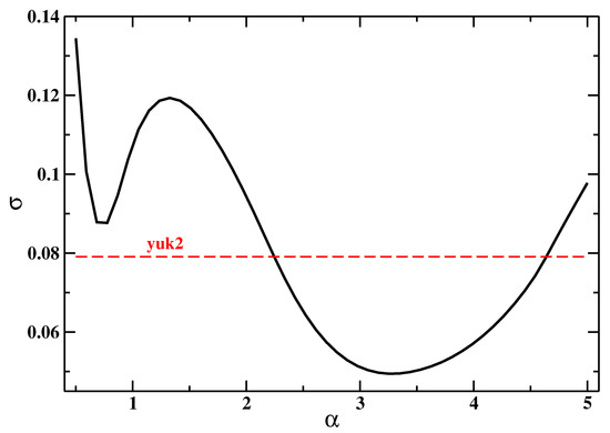
Figure 1.
Values of the error function (Equation (63)) for the function for different values of the parameter. For comparison, the value corresponding to the yuk2 functional, ref. [71] is also reported.
The linear response functions for various cases are reported in Figure 2. Inspection of the plot shows that they are all quite similar, as already suggested by the considerations above. For , we obtain at , where the Lindhard function shows a derivative singularity, that , which is very close to the exact value [5]. Actually, it is also possible also to satisfy exactly using , even if the global accuracy is somehow smaller in this case ().
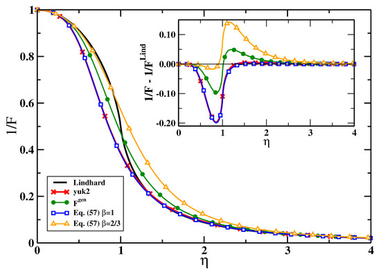
Figure 2.
Linear response functions as computed by Equations (55) and (62) [] for . For Equation (55), two different choices of have been considered; for each one, the value of has been chosen such to minimize the error in Equation (63). The exact Lindhard and the yuk2 responses are also reported for comparison. The inset shows instead the difference between the Lindhard function and the various response functions reported in the plot.
3. Linear yGGA Functionals
We consider the simplest case of yGGA functional by taking functionals that have an enhancement factor with the general form
i.e., a linear dependence on y. Note that these are closely related with the yGGAs defined in Ref. [71], which are recovered if and . However, in this work, we lift this restriction.
From Equation (65), we have that is satisfied by construction if and , , , , , where we have used the short-hand notation , and . Using Equations (50)–(53), we then obtain
The simplest functional satisfying these conditions is the one with
Equation (68) has been derived from Equation (54) using the fact that, for functionals defined by Equation (65), . The Equations (65), (68), and (69) define the yuk2 functional, which reproduces the Lindhard functional at small up to fourth order and for large behaves as
Although the exact value can be obtained for specific values of and , this condition does not have a big impact on the overall accuracy of the linear response. We consider the general error indicator of the linear response of yuk2 with respect to the Lindhard function (Equation (63)). Results for different values of the and are reported as a colormap in Figure 3.
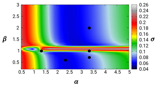
We find that, as seen in the previous section, there is a quite broad range of values that yield small errors (blue areas in the plot). Moreover, the errors are almost independent on , except for values , where a discontinuity in the linear response behavior occurs.
Moreover, from the results of the previous section, we can fix , such that , which is shown in Figure 4.
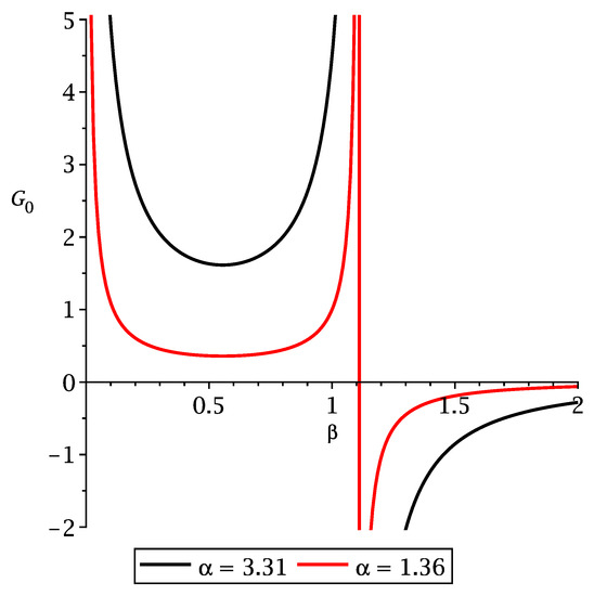
Figure 4.
Value of as a function of for different values of .
Note that is positive up to , where it has a pole, and it has a minimum at . We remark that instead setting and , then Equation (68) readily yields . Thus, the yuk2 functional immediately reduces to the yuk2 functional of Ref. [71].
The yuk2 functional is just a simple ansatz recovering an accurate linear response behavior. However, because it uses a linear dependence on p and q, it may display severe drawbacks in real applications. In particular, the positivity of the Pauli KE density must be ensured [38,92], which is not the case for Equation (65). In fact, the quantity
is not always positive. Thus, we define the yuk3 functional as
with being a positive function such that for , we have , such as the one considered in Ref. [71]. Thus, lacking any quadratic term, the yuk3 has the same linear response of yuk2. In this way, although the functional is not truly a linear function of y, it practically behaves as a linear function of y because . True non-linear yGGA functionals, with , are much more complicated, and they will be considered elsewhere.
4. Computational Details
Densities and enhancement factors were computed in post-SCF fashion using the orbitals of self-consistent Kohn–Sham calculations. All Kohn–Sham calculations have been performed using an in-house developed code solving numerically the spherical symmetry Kohn–Sham problem with the local density approximation being used for the exchange-correlation functional.
Neutral jellium spheres with = 40, 92, 254 electrons and Wigner–Seitz radius = 2, 3, 4, 5, and 6 were considered. They are characterized by the positive background density
The post-processing of the Kohn–Sham orbitals to obtain the quantities , y, and w has been carried out by an additional in-house software which evaluates the required derivatives and integrals in real space using the same grid as the one used in the Kohn–Sham calculations.
5. Results
We considered different pairs of and values for the y ingredient, as reported in Table 1 (see also Figure 3). The first pair (, ) is the one of the original yuk2 functional of Ref. [71]. The second, third, and fourth pairs consider the value suggested by Figure 1 and several values of . The last pair considers the minimizing value of Figure 4 and a corresponding such that . All these pairs give a quite accurate description of the HEG linear response: the highest accuracy is obtained for (3.31, 2) and (2.34, 5/9), as reported in the last column of Table 1.

In Figure 5, we report, in panels (a), (b), (c) and (d) respectively, the electronic density, the function x defined in Equation (68), as well as the values of y and w for a jellium sphere with electrons and .
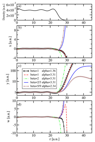
Figure 5.
Electronic density (a) and KE ingredients (b–d) for a jellium sphere with electrons and . The ingredients x, y, and w are reported for different choices of the and parameters.
Looking at Figure 5, we see in panel (b) that for , the values of x are negative in the tail, as also discussed in Appendix C. Moreover, panel (c) shows that the ingredient y is close to 1 inside the jellium spheres for all (,) pairs but in the tail, it diverges for . On the other hand, for , it reaches a constant (but it will slowly vanish in very far regions), while for , it soon decreases to zero, as discussed in Section 2. Finally, panel (d) shows the ingredient w. Inside the sphere, the values of w are in the range for all the , ) combinations. The behavior in the tail follows the one of x but for and , there is a peak before the negative divergence.
These results indicate that for the total kinetic energy, which is mainly influenced by the functional behavior inside the jellium sphere, all the cases considered here can be expected to yield similar results, which are in line with the performance of the yuk3 functional [71]. On the other hand, for the potential, we have a contribution . However, this latter term for functionals with is largely divergent ( is diverging but is not); similarly, it diverges in the (, ) case, where w strongly oscillates around bohr. Thus, we can expect, for these values of the parameters, major problems on the KE potential.
To understand better the role of on the KE functional, we can perform a further analysis of the “exact” Pauli KE enhancement factor
where is the Pauli KE density corresponding to the Kohn–Sham positive-defined KE density and is the Thomas–Fermi density. Hence, we have computed for several jellium clusters with different numbers of electrons () and = 2, 3, 4, 5, and 6 on all grid points, and we have plotted it versus the corresponding values of w. In fact, Equation (73) implies that that the Pauli enhancement factor can be written as a universal single-valued function of w. However, this is an ansatz, which must be verified; if it is correct, then we must obtain a unique value of for each w, also for different systems.
Figure 6 shows the plot of vs. w for the various pairs of parameters considered in this work. It is evident that the cases with and the case with (, ) do not yield single-valued functions but rather display multiple branches of for all values of w. This confirms that using these parameters, it is not possible to obtain an accurate description of the kinetic functional. On the contrary, the yuk2 parameterization (, ) and the one with (, ) show a nice single line for . For negative w values, they display a multi-valued behavior; however, for these cases, the region corresponds to the density tail region. Therefore, the effect, at least on the computation of the energy, is minor. Thus, we can infer that both functionals will be accurate for the kinetic energies (this is indeed the case for yuk2 [71]) but may yield some oscillations in the asymptotic part of the potential because of the multi-valued behavior at . This latter feature is possibly significantly reduced for (, ) that displays the lowest grade of multi-valuedness at negative w values.
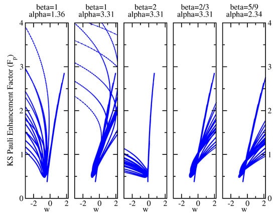
Figure 6.
Exact Pauli Kohn–Sham enhancement factor (Equation (75)) vs. the w ingredient as computed on all grid points for several jellium spheres (see text for details). Each panel corresponds to a different choice of the and parameters.
In a future work, we will develop an approach that will allow us to obtain an analytical function in order to build up an accurate KE functional and KE potential. However, the results reported in Figure 6 also indicate that the ansatz in Equation (73) may be not accurate enough and further studies are required, in particular, to investigate the effect of the non-linear term (), which is already important for the HEG linear-response and can be even more important for the description of finite systems.
6. Conclusions
In this paper, we have investigated non-interacting kinetic energy functionals depending on a generalized Yukawa potential, i.e., a screened Coulomb potential of the electronic density raised to the power of . The use of this input ingredient allows us to introduce in an efficient way non-local features into the functional.
In particular, we have derived the exact homogeneous electron gas linear response behavior of generalized yGGA functionals and, by comparing to the Lindhard function, we have derived exact asymptotic constraints for the functional.
In particular, it turned out that is a very special case, and the Lindhard asymptotic constraints can only be satisfied for a specific value of the screening parameter (). Moreover, the final linear response of yGGA functionals satisfying the low and high-wavevector Lindhard properties does not depend on , which can be then used as an additional degree of freedom to model systems beyond the linear-response regime.
We have used the developed theory to extend the work reported in Ref. [71] and investigate in detail the simplest class of yGGA functionals, namely the linear yGGAs, i.e., those yGGA functionals depending only linearly on y. We have found that although this class of functionals can satisfy rather accurately the linear response constraints, it is not flexible enough to perform very accurately for both the kinetic energy and potential computation. This is mainly due to the fact that imposing the linear response behavior implies, in these simple functionals, that the Pauli enhancement factor is a function of a well-defined combination of the density ingredients (the w ingredient of Equation (72)), but this is not sufficient to describe the non-local nature of the Pauli kinetic energy. Although for some wise choices of the parameters, this effect can be minimized; this is an intrinsic limitation of the linear yGGA functional class.
Therefore, future work will focus on the development of more sophisticated functionals forms using an explicit non-linear dependence on the Yukawa potential. The theoretical framework established in this paper will possibly allow us to develop more efficient and broadly applicable kinetic energy functionals.
Author Contributions
Conceptualization and methodology, E.F. and F.D.S.; software, F.S.; investigation, E.F., F.S. and F.D.S.; writing, E.F., F.S., L.A.C. and F.D.S. All authors have read and agreed to the published version of the manuscript.
Funding
This research received no external funding.
Data Availability Statement
Data sharing is not applicable to this article.
Conflicts of Interest
The authors declare no conflict of interest.
Appendix A. Weak Perturbation of y
To compute the perturbation of y defined in Equation (15), we first consider the generalized Yukawa potential
where we have set . Upon the density perturbation, this becomes
Expanding in series and keeping only terms up to second order, we find
with
Substituting the values of the integrals (see Appendix B), we find
Now, we can consider the perturbation of y, that is
Using the result of Equation (A9) and expanding to second-order, we find
Appendix B. Integrals for the Generalized Yukawa Expansion
For integral , and , we use that
Thus, , , .
To compute the , , and integrals, we can choose the axis such that is aligned with the z axis; then, we have that . Hence, we can write
Thus, and .
The integral is similar to the integral with the substitution . Then,
Appendix C. Asymptotics
For an exponential spherical density , where , we have
so that
Thus, is negative in the tail; i.e., q is very large in the tail but smaller than p. If we consider with , then will be more negative. If we consider with , then will be positive.
References
- Hohenberg, P.; Kohn, W. Inhomogeneous Electron Gas. Phys. Rev. 1964, 136, B864–B871. [Google Scholar] [CrossRef] [Green Version]
- Dreizler, R.M.; Gross, E.K.U. Density Functional Theory; Springer: Berlin/Heidelberg, Germany, 1990. [Google Scholar]
- Levy, M. Universal variational functionals of electron densities, first-order density matrices, and natural spin-orbitals and solution of the v-representability problem. Proc. Nat. Acad. Sci. USA 1979, 76, 6062–6065. [Google Scholar] [CrossRef] [PubMed] [Green Version]
- Kohn, W.; Sham, L.J. Self-Consistent Equations Including Exchange and Correlation Effects. Phys. Rev. 1965, 140, A1133–A1138. [Google Scholar] [CrossRef] [Green Version]
- Wang, Y.A.; Carter, E.A. Orbital-free kinetic-energy density functional theory. In Theoretical Methods in Condensed Phase Chemistry; Springer: Berlin/Heidelberg, Germany, 2002; pp. 117–184. [Google Scholar]
- Wesolowski, T.A.; Wang, Y.A. (Eds.) Recent Progress in Orbital-Free Density Functional Theory; World Scientific: Singapore, 2013. [Google Scholar] [CrossRef] [Green Version]
- Gavini, V.; Bhattacharya, K.; Ortiz, M. Quasi-continuum orbital-free density-functional theory: A route to multi-million atom non-periodic DFT calculation. J. Mech. Phys. Sol. 2007, 55, 697–718. [Google Scholar] [CrossRef]
- Witt, W.C.; Beatriz, G.; Dieterich, J.M.; Carter, E.A. Orbital-free density functional theory for materials research. J. Mater. Res. 2018, 33, 777–795. [Google Scholar] [CrossRef]
- Götz, A.W.; Beyhan, S.M.; Visscher, L. Performance of Kinetic Energy Functionals for Interaction Energies in a Subsystem Formulation of Density Functional Theory. J. Chem. Theory Comput. 2009, 5, 3161–3174. [Google Scholar] [CrossRef]
- Jacob, C.R.; Neugebauer, J. Subsystem density-functional theory. Wiley Interdiscip. Rev. Comput. Mol. Sci. 2014, 4, 325–362. [Google Scholar] [CrossRef]
- Wesolowski, T.A.; Shedge, S.; Zhou, X. Frozen-Density Embedding Strategy for Multilevel Simulations of Electronic Structure. Chem. Rev. 2015, 115, 5891–5928. [Google Scholar] [CrossRef] [Green Version]
- Neugebauer, J. Chromophore-specific theoretical spectroscopy: From subsystem density functional theory to mode-specific vibrational spectroscopy. Phys. Rep. 2010, 489, 1–87. [Google Scholar] [CrossRef]
- Krishtal, A.; Sinha, D.; Genova, A.; Pavanello, M. Subsystem density-functional theory as an effective tool for modeling ground and excited states, their dynamics and many-body interactions. J. Phys. Condens. Matter 2015, 27, 183202. [Google Scholar] [CrossRef]
- Laricchia, S.; Fabiano, E.; Della Sala, F. Frozen density embedding with hybrid functionals. J. Chem. Phys. 2010, 133, 164111. [Google Scholar] [CrossRef] [PubMed]
- Śmiga, S.; Fabiano, E.; Laricchia, S.; Constantin, L.A.; Della Sala, F. Subsystem density functional theory with meta-generalized gradient approximation exchange-correlation functionals. J. Chem. Phys. 2015, 142, 154121. [Google Scholar] [CrossRef] [Green Version]
- Toscano, G.; Straubel, J.; Kwiatkowski, A.; Rockstuhl, C.; Evers, F.; Xu, H.; Asger Mortensen, N.; Wubs, M. Resonance Shifts and Spill-out Effects in Self-Consistent Hydrodynamic Nanoplasmonics. Nat. Commun. 2015, 6, 7132. [Google Scholar] [CrossRef] [PubMed] [Green Version]
- Ciracì, C.; Della Sala, F. Quantum hydrodynamic theory for plasmonics: Impact of the electron density tail. Phys. Rev. B 2016, 93, 205405. [Google Scholar] [CrossRef] [Green Version]
- Moldabekov, Z.A.; Bonitz, M.; Ramazanov, T.S. Theoretical Foundations of Quantum Hydrodynamics for Plasmas. Phys. Plasmas 2018, 25, 031903. [Google Scholar] [CrossRef]
- Baghramyan, H.M.; Della Sala, F.; Ciracì, C. Laplacian-Level Quantum Hydrodynamic Theory for Plasmonics. Phys. Rev. X 2021, 11, 011049. [Google Scholar] [CrossRef]
- Mejia-Rodriguez, D.; Trickey, S.B. Deorbitalization strategies for meta-generalized-gradient-approximation exchange-correlation functionals. Phys. Rev. A 2017, 96, 052512. [Google Scholar] [CrossRef] [Green Version]
- Mejia-Rodriguez, D.; Trickey, S.B. Deorbitalized meta-GGA exchange-correlation functionals in solids. Phys. Rev. B 2018, 98, 115161. [Google Scholar] [CrossRef] [Green Version]
- Mejía-Rodríguez, D.; Trickey, S.B. Meta-GGA performance in solids at almost GGA cost. Phys. Rev. B 2020, 102, 121109. [Google Scholar] [CrossRef]
- Tran, F.; Kovács, P.; Kalantari, L.; Madsen, G.K.H.; Blaha, P. Orbital-free approximations to the kinetic-energy density in exchange-correlation MGGA functionals: Tests on solids. J. Chem. Phys. 2018, 149, 144105. [Google Scholar] [CrossRef] [Green Version]
- Tran, F.; Baudesson, G.; Carrete, J.; Madsen, G.K.H.; Blaha, P.; Schwarz, K.; Singh, D.J. Shortcomings of meta-GGA functionals when describing magnetism. Phys. Rev. B 2020, 102, 024407. [Google Scholar] [CrossRef]
- Acharya, P.K.; Bartolotti, L.J.; Sears, S.B.; Parr, R.G. An atomic kinetic energy functional with full Weizsacker correction. Proc. Nat. Acad. Sci. USA 1980, 77, 6978–6982. [Google Scholar] [CrossRef] [PubMed] [Green Version]
- Thakkar, A.J. Comparison of kinetic-energy density functionals. Phys. Rev. A 1992, 46, 6920. [Google Scholar] [CrossRef]
- Lembarki, A.; Chermette, H. Obtaining a gradient–corrected kinetic–energy functional from the Perdew–Wang exchange functional. Phys. Rev. A 1994, 50, 5328. [Google Scholar] [CrossRef]
- Tran, F.; Wesołowski, T.A. Link between the kinetic-and exchange-energy functionals in the generalized gradient approximation. Int. J. Quant. Chem. 2002, 89, 441–446. [Google Scholar] [CrossRef]
- Constantin, L.A.; Fabiano, E.; Laricchia, S.; Della Sala, F. Semiclassical neutral atom as a reference system in density functional theory. Phys. Rev. Lett. 2011, 106, 186406. [Google Scholar] [CrossRef]
- Laricchia, S.; Fabiano, E.; Constantin, L.A.; Della Sala, F. Generalized Gradient Approximations of the Noninteracting Kinetic Energy from the Semiclassical Atom Theory: Rationalization of the Accuracy of the Frozen Density Embedding Theory for Nonbonded Interactions. J. Chem. Theory Comput. 2011, 7, 2439–2451. [Google Scholar] [CrossRef]
- Karasiev, V.V.; Chakraborty, D.; Shukruto, O.A.; Trickey, S.B. Nonempirical generalized gradient approximation free-energy functional for orbital-free simulations. Phys. Rev. B 2013, 88, 161108(R). [Google Scholar] [CrossRef] [Green Version]
- Borgoo, A.; Tozer, D.J. Density scaling of noninteracting kinetic energy functionals. J. Chem. Theory Comput. 2013, 9, 2250–2255. [Google Scholar] [CrossRef]
- Trickey, S.B.; Karasiev, V.V.; Chakraborty, D. Comment on “Single-point kinetic energy density functionals: A pointwise kinetic energy density analysis and numerical convergence investigation”. Phys. Rev. B 2015, 92, 117101. [Google Scholar] [CrossRef] [Green Version]
- Xia, J.; Carter, E.A. Reply to “Comment on ‘Single-point kinetic energy density functionals: A pointwise kinetic energy density analysis and numerical convergence investigation’”. Phys. Rev. B 2015, 92, 117102. [Google Scholar] [CrossRef] [Green Version]
- Constantin, L.A.; Fabiano, E.; Śmiga, S.; Della Sala, F. Jellium-with-gap model applied to semilocal kinetic functionals. Phys. Rev. B 2017, 95, 115153. [Google Scholar] [CrossRef] [Green Version]
- Luo, K.; Karasiev, V.V.; Trickey, S. A simple generalized gradient approximation for the noninteracting kinetic energy density functional. Phys. Rev. B 2018, 98, 041111(R). [Google Scholar] [CrossRef] [Green Version]
- Lehtomäki, J.; Lopez-Acevedo, O. Semilocal kinetic energy functionals with parameters from neutral atoms. Phys. Rev. B 2019, 100, 165111. [Google Scholar] [CrossRef] [Green Version]
- Perdew, J.P.; Constantin, L.A. Laplacian-level density functionals for the kinetic energy density and exchange-correlation energy. Phys. Rev. B 2007, 75, 155109. [Google Scholar] [CrossRef] [Green Version]
- Karasiev, V.V.; Jones, R.S.; Trickey, S.B.; Harris, F.E. Properties of constraint-based single-point approximate kinetic energy functionals. Phys. Rev. B 2009, 80, 245120. [Google Scholar] [CrossRef] [Green Version]
- Laricchia, S.; Constantin, L.A.; Fabiano, E.; Della Sala, F. Laplacian-Level kinetic energy approximations based on the fourth-order gradient expansion: Global assessment and application to the subsystem formulation of density functional theory. J. Chem. Theory Comput. 2013, 10, 164–179. [Google Scholar] [CrossRef] [Green Version]
- Cancio, A.C.; Stewart, D.; Kuna, A. Visualization and analysis of the Kohn-Sham kinetic energy density and its orbital-free description in molecules. J. Chem. Phys. 2016, 144, 084107. [Google Scholar] [CrossRef] [Green Version]
- Cancio, A.C.; Redd, J.J. Visualisation and orbital-free parametrisation of the large-Z scaling of the kinetic energy density of atoms. Mol. Phys. 2017, 115, 618–635. [Google Scholar] [CrossRef] [Green Version]
- Constantin, L.A.; Fabiano, E.; Della Sala, F. Semilocal Pauli–Gaussian Kinetic Functionals for Orbital-Free Density Functional Theory Calculations of Solids. J. Phys. Chem. Lett. 2018, 9, 4385–4390. [Google Scholar] [CrossRef] [Green Version]
- Constantin, L.A.; Fabiano, E.; Della Sala, F. Performance of Semilocal Kinetic Energy Functionals for Orbital-Free Density Functional Theory. J. Chem. Theory Comput. 2019, 15, 3044–3055. [Google Scholar] [CrossRef] [PubMed]
- Śmiga, S.; Constantin, L.A.; Della Sala, F.; Fabiano, E. The Role of the Reduced Laplacian Renormalization in the Kinetic Energy Functional Development. Computation 2019, 7, 65. [Google Scholar] [CrossRef] [Green Version]
- Xia, J.; Carter, E.A. Single-point kinetic energy density functionals: A pointwise kinetic energy density analysis and numerical convergence investigation. Phys. Rev. B 2015, 91, 045124. [Google Scholar] [CrossRef] [Green Version]
- Wang, L.W.; Teter, M.P. Kinetic-energy functional of the electron density. Phys. Rev. B 1992, 45, 13196. [Google Scholar] [CrossRef]
- Perrot, F. Hydrogen-hydrogen interaction in an electron gas. J. Phys. Condens. Matter 1994, 6, 431. [Google Scholar] [CrossRef]
- Smargiassi, E.; Madden, P.A. Orbital-free kinetic-energy functionals for first-principles molecular dynamics. Phys. Rev. B 1994, 49, 5220. [Google Scholar] [CrossRef]
- García-González, P.; Alvarellos, J.E.; Chacón, E. Nonlocal kinetic-energy-density functionals. Phys. Rev. B 1996, 53, 9509. [Google Scholar] [CrossRef]
- García-González, P.; Alvarellos, J.E.; Chacón, E. Kinetic-energy density functional: Atoms and shell structure. Phys. Rev. A 1996, 54, 1897. [Google Scholar] [CrossRef]
- García-González, P.; Alvarellos, J.E.; Chacón, E. Nonlocal symmetrized kinetic-energy density functional: Application to simple surfaces. Phys. Rev. B 1998, 57, 4857. [Google Scholar] [CrossRef]
- Wang, Y.A.; Govind, N.; Carter, E.A. Orbital-free kinetic-energy functionals for the nearly free electron gas. Phys. Rev. B 1998, 58, 13465. [Google Scholar] [CrossRef] [Green Version]
- Wang, Y.A.; Govind, N.; Carter, E.A. Orbital-free kinetic-energy density functionals with a density-dependent kernel. Phys. Rev. B 1999, 60, 16350. [Google Scholar] [CrossRef] [Green Version]
- Zhou, B.; Ligneres, V.L.; Carter, E.A. Improving the orbital-free density functional theory description of covalent materials. J. Chem. Phys. 2005, 122, 044103. [Google Scholar] [CrossRef]
- Garcia-Aldea, D.; Alvarellos, J. Fully nonlocal kinetic energy density functionals: A proposal and a general assessment for atomic systems. J. Chem. Phys. 2008, 129, 074103. [Google Scholar] [CrossRef]
- Garcia-Aldea, D.; Alvarellos, J.E. Approach to kinetic energy density functionals: Nonlocal terms with the structure of the von Weizsäcker functional. Phys. Rev. A 2008, 77, 022502. [Google Scholar] [CrossRef]
- Huang, C.; Carter, E.A. Nonlocal orbital-free kinetic energy density functional for semiconductors. Phys. Rev. B 2010, 81, 045206. [Google Scholar] [CrossRef] [Green Version]
- Shin, I.; Carter, E.A. Enhanced von Weizsäcker Wang-Govind-Carter kinetic energy density functional for semiconductors. J. Chem. Phys. 2014, 140, 18A531. [Google Scholar] [CrossRef]
- Constantin, L.A.; Fabiano, E.; Della Sala, F. Nonlocal kinetic energy functional from the jellium-with-gap model: Applications to orbital-free density functional theory. Phys. Rev. B 2018, 97, 205137. [Google Scholar] [CrossRef] [Green Version]
- Mi, W.; Genova, A.; Pavanello, M. Nonlocal kinetic energy functionals by functional integration. J. Chem. Phys. 2018, 148, 184107. [Google Scholar] [CrossRef] [Green Version]
- Mi, W.; Pavanello, M. Orbital-free density functional theory correctly models quantum dots when asymptotics, nonlocality, and nonhomogeneity are accounted for. Phys. Rev. B 2019, 100, 041105. [Google Scholar] [CrossRef] [Green Version]
- Xu, Q.; Lv, J.; Wang, Y.; Ma, Y. Nonlocal kinetic energy density functionals for isolated systems obtained via local density approximation kernels. Phys. Rev. B 2020, 101, 045110. [Google Scholar] [CrossRef] [Green Version]
- Finzel, K. Shell-structure-based functionals for the kinetic energy. Theor. Chem. Acc. 2015, 134, 106. [Google Scholar] [CrossRef]
- Finzel, K. Local conditions for the Pauli potential in order to yield self-consistent electron densities exhibiting proper atomic shell structure. J. Chem. Phys. 2016, 144, 034108. [Google Scholar] [CrossRef] [PubMed] [Green Version]
- Ludeña, E.V.; Salazar, E.X.; Cornejo, M.H.; Arroyo, D.E.; Karasiev, V.V. The Liu-Parr power series expansion of the Pauli kinetic energy functional with the incorporation of shell-inducing traits: Atoms. Int. J. Quantum Chem. 2018, 118, e25601. [Google Scholar] [CrossRef]
- Salazar, E.X.; Guarderas, P.F.; Ludena, E.V.; Cornejo, M.H.; Karasiev, V.V. Study of some simple approximations to the non-interacting kinetic energy functional. Int. J. Quantum Chem. 2016, 116, 1313–1321. [Google Scholar] [CrossRef] [Green Version]
- Yao, K.; Parkhill, J. Kinetic Energy of Hydrocarbons as a Function of Electron Density and Convolutional Neural Networks. J. Chem. Theory Comput. 2016, 12, 1139–1147. [Google Scholar] [CrossRef]
- Alonso, J.A.; Girifalco, L.A. Nonlocal approximation to the exchange potential and kinetic energy of an inhomogeneous electron gas. Phys. Rev. B 1978, 17, 3735. [Google Scholar] [CrossRef]
- Chacón, E.; Alvarellos, J.E.; Tarazona, P. Nonlocal kinetic energy functional for nonhomogeneous electron systems. Phys. Rev. B 1985, 32, 7868. [Google Scholar] [CrossRef]
- Sarcinella, F.; Fabiano, E.; Constantin, L.A.; Della Sala, F. Nonlocal kinetic energy functionals in real space using a Yukawa-potential kernel: Properties, linear response, and model functionals. Phys. Rev. B 2021, 103, 155127. [Google Scholar] [CrossRef]
- Kumar, S.; Borda, E.L.; Sadigh, B.; Zhu, S.; Hamel, S.; Gallagher, B.; Bulatov, V.; Klepeis, J.; Samanta, A. Accurate parameterization of the kinetic energy functional. J. Chem. Phys. 2022, 156, 024110. [Google Scholar] [CrossRef]
- Karasiev, V.V.; Chakraborty, D.; Trickey, S.B. Progress on New Approaches to Old Ideas: Orbital-Free Density Functionals. In Many-Electron Approaches in Physics, Chemistry and Mathematics; Bach, V., Delle Site, L., Eds.; Springer: Cham, Switzerland, 2014; pp. 113–134. [Google Scholar] [CrossRef]
- March, N.; Santamaria, R. Non-local relation between kinetic and exchange energy densities in Hartree–Fock theory. Int. J. Quantum Chem. 1991, 39, 585–592. [Google Scholar] [CrossRef]
- Della Sala, F.; Fabiano, E.; Constantin, L.A. Kohn-Sham kinetic energy density in the nuclear and asymptotic regions: Deviations from the von Weizsäcker behavior and applications to density functionals. Phys. Rev. B 2015, 91, 035126. [Google Scholar] [CrossRef] [Green Version]
- Howard, I.A.; March, N.H.; Van Doren, V.E. r- and p-space electron densities and related kinetic and exchange energies in terms of s states alone for the leading term in the 1/Z expansion for nonrelativistic closed-shell atomic ions. Phys. Rev. A 2001, 63, 062501. [Google Scholar] [CrossRef]
- Constantin, L.A.; Fabiano, E.; Della Sala, F. Kinetic and Exchange Energy Densities near the Nucleus. Computation 2016, 4, 19. [Google Scholar] [CrossRef] [Green Version]
- Śmiga, S.; Siecińska, S.; Fabiano, E. Methods to generate reference total and Pauli kinetic potentials. Phys. Rev. B 2020, 101, 165144. [Google Scholar] [CrossRef]
- Snyder, J.C.; Rupp, M.; Hansen, K.; Müller, K.R.; Burke, K. Finding density functionals with machine learning. Phys. Rev. Lett. 2012, 108, 253002. [Google Scholar] [CrossRef]
- Li, L.; Snyder, J.C.; Pelaschier, I.M.; Huang, J.; Niranjan, U.N.; Duncan, P.; Rupp, M.; Müller, K.R.; Burke, K. Understanding machine-learned density functionals. Int. J. Quant. Chem. 2016, 116, 819–833. [Google Scholar] [CrossRef] [Green Version]
- Alharbi, F.H.; Kais, S. Kinetic energy density for orbital-free density functional calculations by axiomatic approach. Int. J. Quantum Chem. 2017, 117, e25373. [Google Scholar] [CrossRef]
- Seino, J.; Kageyama, R.; Fujinami, M.; Ikabata, Y.; Nakai, H. Semi-local machine-learned kinetic energy density functional with third-order gradients of electron density. J. Chem. Phys. 2018, 148, 241705. [Google Scholar] [CrossRef]
- Golub, P.; Manzhos, S. Kinetic energy densities based on the fourth order gradient expansion: Performance in different classes of materials and improvement via machine learning. Phys. Chem. Chem. Phys. 2019, 21, 378–395. [Google Scholar] [CrossRef] [Green Version]
- Manzhos, S.; Golub, P. Data-driven kinetic energy density fitting for orbital-free DFT: Linear vs Gaussian process regression. J. Chem. Phys. 2020, 153, 074104. [Google Scholar] [CrossRef]
- Meyer, R.; Weichselbaum, M.; Hauser, A.W. Machine Learning Approaches toward Orbital-free Density Functional Theory: Simultaneous Training on the Kinetic Energy Density Functional and Its Functional Derivative. J. Chem. Theory Comput. 2020, 16, 5685–5694. [Google Scholar] [CrossRef] [PubMed]
- Imoto, F.; Imada, M.; Oshiyama, A. Order-N orbital-free density-functional calculations with machine learning of functional derivatives for semiconductors and metals. Phys. Rev. Res. 2021, 3, 033198. [Google Scholar] [CrossRef]
- Ryczko, K.; Wetzel, S.J.; Melko, R.G.; Tamblyn, I. Toward Orbital-Free Density Functional Theory with Small Data Sets and Deep Learning. J. Chem. Theory Comput. 2022, 18, 1122–1128. [Google Scholar] [CrossRef] [PubMed]
- Prodan, E.; Kohn, W. Nearsightedness of electronic matter. Proc. Nat. Acad. Sci. USA 2005, 102, 11635–11638. [Google Scholar] [CrossRef] [Green Version]
- Constantin, L.A.; Fabiano, E.; Della Sala, F. Modified Fourth-Order Kinetic Energy Gradient Expansion with Hartree Potential-Dependent Coefficients. J. Chem. Theory Comput. 2017, 13, 4228–4239. [Google Scholar] [CrossRef]
- Lindhard, J. On the properties of a gas of charged particles. Dan. Vid. Selsk Mat.-Fys. Medd. 1954, 28, 8. [Google Scholar]
- Tao, J.; Perdew, J.P.; Almeida, L.M.; Fiolhais, C.; Kümmel, S. Nonempirical density functionals investigated for jellium: Spin-polarized surfaces, spherical clusters, and bulk linear response. Phys. Rev. B 2008, 77, 245107. [Google Scholar] [CrossRef]
- Levy, M.; Ou-Yang, H. Exact properties of the Pauli potential for the square root of the electron density and the kinetic energy functional. Phys. Rev. A 1988, 38, 625–629. [Google Scholar] [CrossRef]
Publisher’s Note: MDPI stays neutral with regard to jurisdictional claims in published maps and institutional affiliations. |
© 2022 by the authors. Licensee MDPI, Basel, Switzerland. This article is an open access article distributed under the terms and conditions of the Creative Commons Attribution (CC BY) license (https://creativecommons.org/licenses/by/4.0/).