1. Introduction
Number comparison and sign detection are simple and basic operations for calculation in computing systems. Both operations are necessary for almost any application area in computing technology: mathematical calculations, rendering, data storage, data transfer, data retrieval, encryption, machine learning, etc. Unfortunately, their application for encrypted data exhibits several limitations.
Sign detection and comparison of numbers in the Residue Number System (RNS) are based on the calculation of the positional characteristic. The algorithms for both operations in RNS are computationally complex because RNS is not a Weighted Number System (WNS). Various methods are used to reduce their computational complexity, such as the Pirlo and Impedovo function [
1], Diagonal Function (DF) [
2,
3], Modified Diagonal Function (MDF) [
4], Approximate Method (AM) [
5,
6], and Core Function (CF) [
7].
Both operations are fundamental for the applicability of RNS for both hardware and software implementations. Reducing their computational complexity expands the scope of RNS for solving problems of computational mathematics and mathematical modeling. For instance, the use of RNS in software implementation on the GPU increases the performance of matrix processing [
8,
9]. Moreover, RNS is a main direction in the implementation of Homomorphic Encryption (HE) software.
Fully HE (FHE) has gained popularity for its applicability in cryptosystems [
10]. Performing simple arithmetic operations (homomorphic addition and multiplication) over ciphertexts is its main feature. Hence, the processing of encrypted information does not require its preliminary decryption. This characteristic increases the confidentiality and reliability of the data processing [
11,
12], for example, in third-party systems such as cloud computing [
13,
14].
However, comparing ciphertext information is a laborious and computationally complex task [
15,
16]. Cheon–Kim–Kim–Song (CKKS) [
17] and Brakerski/Fan–Vercauteren (BFV) [
18] are FHE schemes that use RNS to increase the efficiency of sign detection and numbers’ comparison [
4,
6,
19,
20,
21].
The comparison operation can be performed in a relatively simple way: subtract one number from another, and if the result of the operation is negative, then the first number is greater than the second one and vice versa. Many methods in RNS work using this property. However, they are often ineffective, since they apply division by large numbers or use computationally complex algorithms to calculate the positional characteristic of the number.
In this paper, we consider a new algorithm for determining the sign of numbers in an even range with RNS. The content of the paper is structured as follows.
Section 2 briefly introduces the residue number system.
Section 3 describes several methods to determine the sing of numbers in RNS. The performance evaluation is described in
Section 4. Finally, we conclude and discuss future works in
Section 5.
2. Residue Number System
RNS is a not WNS based on Chinese Remainder Theorem (CRT) [
22,
23]. It is defined by a vector of coprime numbers called moduli. This vector, also called the RNS basis, can be denoted as
. The basis is determined by the product of all the
elements:
, where
is the length of the moduli vector. A positional number
is represented in RNS by the residues
, where
A restriction is imposed on the number such that ; otherwise, the residue of the number will be obtained from the number , where . Additionally, the CRT corollary guarantees the uniqueness of the representation of non-negative integers within the interval . The representation of negative numbers in RNS considers the radix addition, where is represented as . This property is used to determine the sign of a number based on converting a number from RNS to WNS, i.e., decimal, binary, etc.
The simplicity to perform basic arithmetic operations is the main advantage of RNS for computing. Addition, multiplication, and subtraction operations are performed according to the following general formula:
where ∗ denotes operations such as addition, multiplication, and subtraction.
The modular arithmetic, or operations in RNS, has several particularities: the value of the number in each residue does not depend on other residues, and one cycle of the processor’s numerical processing is enough to perform such operations, since this processing can be performed in parallel.
Let us prove that the ranges of numbers in RNS and WNS are equal. For example, for moduli RNS , , , , and , the RNS range is and WNS range is .
Let RNS be given by the basis and the number with residues . Then, the number can be represented in the form.
where is from to , and are the coefficients of RNS.
The ranges of numbers represented in RNS and WNS coincide; i.e., we can talk about the presence of a one-to-one correspondence between the set of number representations in RNS and WNS.
The previous equality can be rewritten as:
thereby translating numbers into WNS. It establishes the basic concepts of RNS, operations, and translating numbers from WNS to RNS and vice versa.
3. Methods for Determining the Sign of a Number in RNS
3.1. Chinese Remainder Theorem
The following formula is used to convert numbers from RNS to WNS with Chinese Remainder Theorem (CRT)
where
and
is a multiplicative inverse of
modulo
.The restored number must be compared with . If , then the number is greater than zero. Two’s complement is the most common method of representing signed integers. Its half of the range (the upper half) denotes a negative number and vice versa. To estimate the time complexity, we assume that all RNS moduli are composed of -bits bit words, so the time complexity is defined by
Let us consider an example based on this method.
Example 1. Let the number be represented in RNS with moduli and residues . Initially, we calculate the dynamic range and the elements:
Then, we compute the multiplicative inverse, which consists in finding
, such that
. Therefore,
Next, we use Formula (2) to calculate the value of
:
Finally, we compare with ; then, or . Therefore, the number is positive.
Algorithm 1 presents the pseudocode of the CRT method.
| Algorithm 1: CRT Method. |
Input: ,
Output:
do:
:
4.1
5. else:
|
However, this method has a significant drawback due to the divisions to obtain . The division of large numbers by a large increases the time required for calculations.
3.2. Mixed Radix Conversion Method
The Mixed Radix Conversion (MRC) method consists of a consecutive translation of a number from RNS to WNS. In addition, a pattern in the number in a generalized form is traced by
, where
is known as the conversion coefficient and defines an increasing series
Yassin and Moore [
24] found that
Example 2. The initial data are a set of moduli , a set of residues , and .
First, we find the
coefficients:
Second, the number is restored by (2)
Finally, we compare with ; then, . Therefore, the number is positive. Time complexity is
Algorithm 2 describes the pseudocode of the MRC method.
| Algorithm 2: MRC Method. |
Input: and
Output:
1. , , , and
2. for to do
2.1
2.2
2.3
3.
4. for to do
4.1
4.2
5
6 if:
6.1
7. else:
|
Effective implementation of this method allows avoiding division by a large . However, the method uses many modular operations related to the vector .
3.3. Approximate Method
The algorithm for finding the Euclidean division by the range RNS is computationally complex. To reduce the computational complexity of the Approximate Method (AM), it is proposed to use weighted coefficients, which allow replacing the operation of Euclidean division with the operation of taking a fractional part.
AM is based on the mapping from to to avoid the division by a large .
The mapping allows calculating the positional characteristic of the number, hence, to determine the sign of the number or compare numbers with each other. The positional characteristic is originally calculated as:
However, the use of (3) as a positional characteristic requires the use of rational fractions or their approximation using numbers with a fixed precision, which increases the computational complexity of the algorithm. In [
25], a modification of the methods from [
5] was proposed, which allows retaining the advantages of the method from [
5] but at the same time avoiding the use of rational numbers.
where
, with
, and
. If
then
else
. Time complexity is
Example 3. , moduli RNS: , , , , , and .
We calculate the coefficients
:
Thus, we can translate the number based on the coefficients
Therefore, the number is negative because .
Algorithm 3 shows the pseudocode of the AM.
| Algorithm 3: AM Method. |
Input: , and N
Output:
1. for to do
1.1
2
3. if:
3.1
4. else:
|
3.4. Diagonal Function
The positional characteristic of a number in RNS can be also determined by the so-called Diagonal Function (DF), which is defined by
[
2]. To calculate
using moduli RNS, use the following formula:
where
,
.
The sign of the number depends on the comparison of and . Let us look at an example of comparing numbers. The time complexity of the algorithm is
Example 4. We consider the numbers of previous examples, and moduli . First, we calculate the values and .
Then, we find the value of the DF:
Since , then is positive.
Algorithm 4 describes the pseudocode of the DF method.
| Algorithm 4: DF Method. |
Input
Output
do
:
4. else:
|
3.5. Core Function
Burgess [
26] proposed the minimal Akushsky Core Function (CF) based on the result obtained in [
27,
28]. This approach is similar to the DF method, and it does not need to calculate the critical cores.
The analytical form of the Pirlo function is calculated as:
where
If , then the number is positive, since the function under study is monotonically increasing. Time complexity is
Let us consider an example of comparing numbers.
Example 5. We take the numbers of previous examples, and moduli . First, let us calculate the values and as:
Then, we compute the Pirlo function:
Since , the number is positive.
Algorithm 5 describes the pseudocode of the CF method.
| Algorithm 5: CF Method. |
Input
Output
do
:
4. else:
|
3.6. Determining the Sign of a Number
Knowing the sign of a number can increase the performance of number comparison in RNS; the difference between numbers
and
provides information about their comparison. Determining the Sign of a Number (DSN) in RNS is based on the fact that the residues
of the negative number
are the complement of
to the modulus
. Hence, the following relationship holds:
The formula based on CRT and an AM allows determining the sign of the number based on the following equation [
29].
if the equation holds; otherwise,
.
Let us consider the algorithm for comparing numbers in RNS based on DSN.
Example 6. Let the number in RNS be with the basis . We determine the sign of the number by calculating Formula (8):
So, the number is positive.
Algorithm 6 shows the pseudocode of the DSN method.
| Algorithm 6: DSN Method. |
Input
Output
do:
:
4. else:
|
3.7. Modified Diagonal Function
The Modified Diagonal Function (MDF) method reduces the computational complexity of comparing numbers in the RNS [
5]. It proposes a new positional characteristic based on the DF and an AM. The essence of the MDF method is to calculate the relative value of the DF to
, which allows replacing the computationally complex operation of finding the residue of division by
by taking the fractional part of the number, and the coefficients
are replaced by the relative value
of
in Formula (5).
where
,
, and
.
Let us look at an example of comparing numbers. Time complexity is
Example 7. We use the previously numbers and moduli . Then, we take and value from the diagonal function:
We find the value of the MDF:
The number is positive, since
. Algorithm 7 shows the pseudocode of the MDF method.
| Algorithm 7: MDF Method. |
Input
Output
do
:
|
3.8. Determining the Sign of a Number in RNS with an Even Range
Here, we propose the efficient method Determining the Sign of a Number (DSN) in RNS with an Even Range (DSN-EN) for comparing numbers and determining the sign of a number for the case of an even RNS range.
Since the RNS range is an Even Number (EN), one of the RNS moduli is an EN. Without loss of generality, we assume that the module is even; then, using the property , the determination of a sign is reduced to a two-stage algorithm.
The first stage is dividing by an integer . The second stage is dividing by an integer .
Formally, it is determined by the following formula:
The correctness of (10) follows from the proof of the following Theorem 1.
Theorem 1. If and are integer numbers with , then the equality holds:
Proof. Due to
, Equality (11) takes the form:
We represent
in the form
. Substituting it in (12), we have:
Let
, where
we obtain:
Considering that
, then
and
Hence,
and
Substituting this result in (13), we have:
The theorem is proved. □
Corollary 1. Equation (10) is correct.
Proof. Let and . Since is an even number, then is an integer number. Therefore, the conditions of Theorem 1 are satisfied and the corollary is proved. The time complexity of the algorithm is . □
Example 8. Let the RNS be given by the moduli and . We determine the sign of a number and . Let us calculate the synoptic weights:
The number
is positive since
and
is negative because
Algorithm 8 shows the pseudocode of the DSN with the EN method.
| Algorithm 8: DSN-EN. |
Input
Output
do
do
1.1.1
:
|
4. Performance Evaluation
The proposed algorithm described in
Section 3.8 has the advantage among the methods described in
Section 3.
To confirm the properties, we implement all the algorithms using the high-level language C++ and compare their performance. The experiments are carried out on operating systems Windows 10 Home Edition on a computer with Intel Core i5-8250U 1.60 GHz, RAM DDR4 8 GB 1196 MHz, and SSD 512 GB.
For the analysis, we use a 128-bit number transferred to RNS, a set of six RNS moduli, and a width of 24 to 64 bits. We vary a vector length of 3 to 8 moduli with a 32-bit width.
The experimental results report the maximum, minimum, and average of 10,000 runs of each method. Additionally, we incorporate the average calculated based on the maximum and minimum values.
The information of the execution is presented in
Appendix A. For simplicity, we only analyze the significant discoveries of the results. The average values have stable linear growth. The minimum values are prevailing because the average values of each method are very close to them. Hence, the maximum values are not common causes.
To avoid time measuring biases, the mean values are calculated as the average of 10,000 measuring of the maximum values and 10,000 measuring of the minimum values. We also consider the medium values of all methods to determine the most efficient ones.
Comparative Analysis
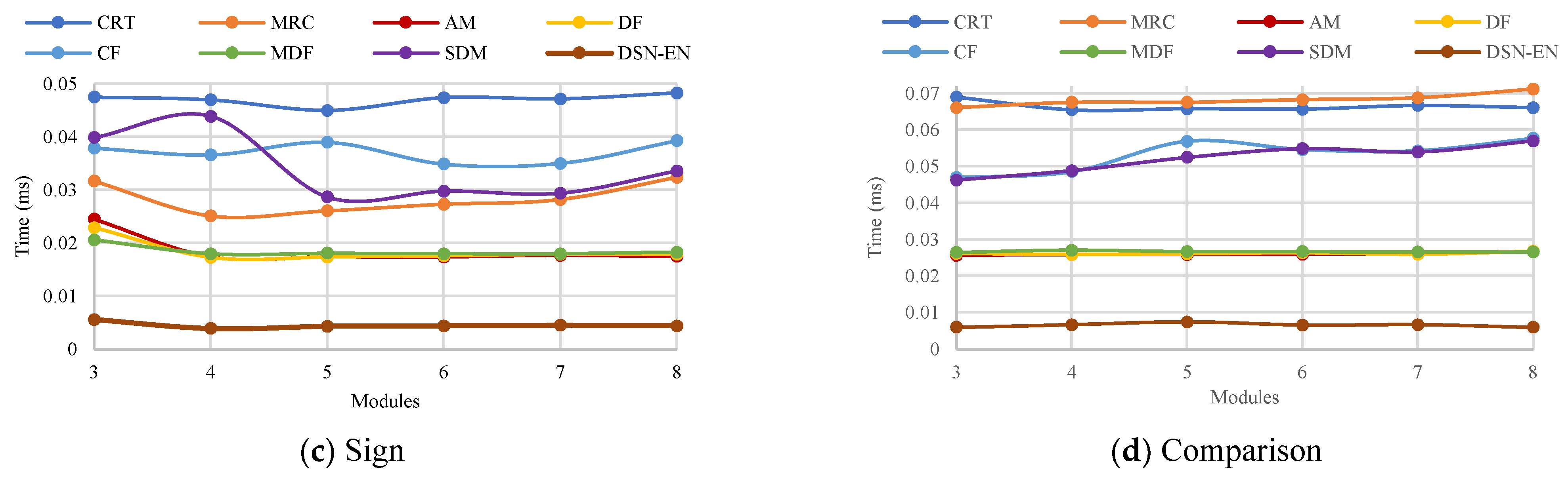
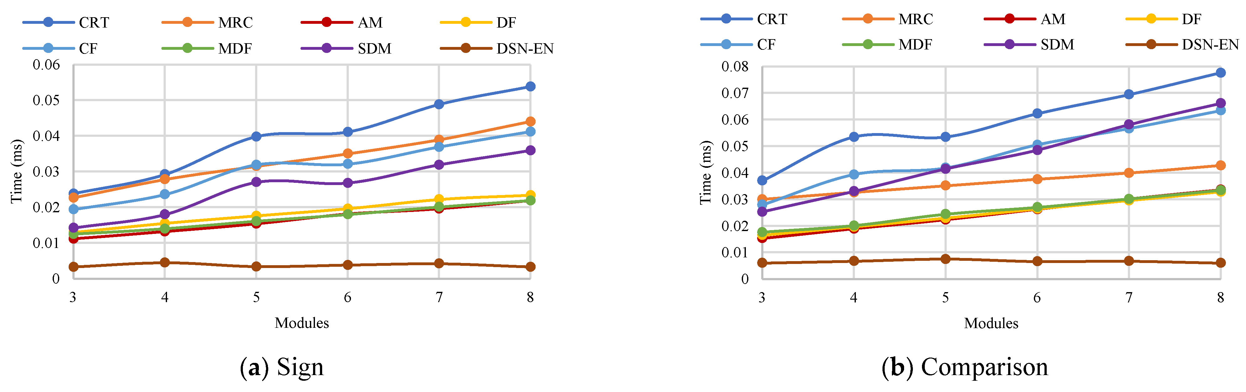
The performance of all methods for the operations of determining the sign of a number and number comparison is presented in
Figure 1. DSN-EN has the highest performance for both operations with different numbers of modules
and dynamic bit width. AM, DF, and MDF are in the group of the second most efficient methods for all operations.
The results with a different number of modules show: Considering the sign detection with respect to DSN-EN, the efficiency of AM is between 1.93 and 5.64 times worst. Likewise, DF and MDF are from 2.44 to 6.1 and from 2.11 to 5.64 times worst, respectively. Similar results present the comparison of numbers, DSN-EN improves AM within 1.55–4.6 times, DF among 1.75–4.47 times, and MDF within 1.93–4.57 times.
The results of comparison with different dynamic bit widths exhibit that DSN-EN is more efficient than MDF from 2.68 to 3.61 times, AM within 2.93–3.46 times, and MD between 2.97 and 3.44 times. For comparison of numbers, the differences are in 2.45–3.47, 2.48–3.47, and 2.56–3.43 for AM, DF, and MDF, respectively.
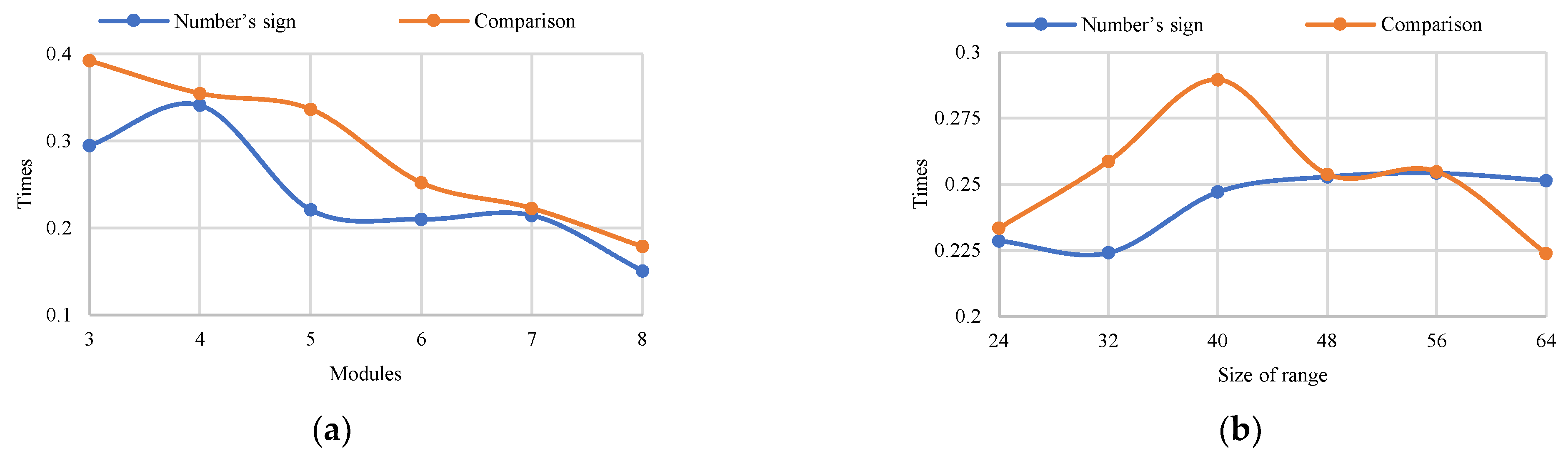
Figure 2 present a comparison between DSN-EN and AM, both methods with the best overall performance. From
Figure 2a, we observe that the time difference is increased with respect to the number of modules for both operations.
Figure 2b shows the execution time varying a dynamic bit width.
In general, the proposed method is several times more productive than AM, which was determined as the most efficient of the existing state-of-the-art ones. We consider that the DSN-EN can be applied efficiently in systems that use RNS.
5. Conclusions
Determining the sign of a number is fundamental for the implementation of several techniques with privacy preserving in untrusted environments. Current homomorphic encryption approaches try to make the implementation of this operation more efficient by using a residual number system. Unfortunately, the methods based on converting a number to a weight number system and determining the sign are inefficient and slow. The calculation of positional characteristics is better in performance but not efficient.
We propose a new method to determine the sign of a number in RNS and provide a theoretical foundation for when one modulo is an even number. We provide its performance evaluation compared with other determining the sign methods. The results show the advantages of our approach for different modules numbers and dynamic bit widths. In the future, we will study determining the sign of a number and comparing numbers in RNS for odd ranges.
Author Contributions
The authors have contributed in different parts of the paper preparation, as follows: Conceptualization, A.T. and M.B.; methodology, A.T., M.B., E.S. and A.A.; software, E.S., B.P.-G. and J.M.C.-M.; validation, E.S., B.P.-G., J.M.C.-M. and V.K.; formal analysis, A.T., M.B., E.S. and A.Y.D.; investigation, A.T., M.B., E.S. and A.A.; resources, E.S., and B.P.-G.; data curation, B.P.-G. and J.M.C.-M.; writing—original draft preparation, A.T., M.B., E.S., A.Y.D. and V.K.; writing—review and editing, A.T., B.P.-G., J.M.C.-M. and A.A.; visualization, B.P.-G. and J.M.C.-M.; supervision, A.T. and M.B.; project administration, A.T. and M.B.; funding acquisition, M.B. All authors have read and agreed to the published version of the manuscript.
Funding
This work was supported by the Ministry of Education and Science of the Russian Federation (Project 075-15-2020-915).
Institutional Review Board Statement
Not applicable.
Informed Consent Statement
Not applicable.
Data Availability Statement
Data is contained within the article.
Conflicts of Interest
The authors declare no conflict of interest.
Appendix A
Table A1 presents the time in milliseconds (ms) needed to determine the number’s sign and comparison of numbers for considered methods with a dynamic number of modules
based on the 10,000 measurements.
Table A1.
Operation time with a dynamic number of modules (ms).
Table A1.
Operation time with a dynamic number of modules (ms).
| Method | Modules | Number’s Sign | Comparison |
|---|
| Max | Mean | Min | Mean–Min | Max | Mean | Min | Mean–Min |
|---|
| CRT | 3 | 0.1130 | 0.0238 | 0.0229 | 0.0009 | 0.1876 | 0.0370 | 0.0355 | 0.0015 |
| 4 | 0.1451 | 0.0292 | 0.0287 | 0.0005 | 0.1562 | 0.0534 | 0.0434 | 0.0100 |
| 5 | 0.1547 | 0.0398 | 0.0381 | 0.0017 | 0.2381 | 0.0534 | 0.0510 | 0.0024 |
| 6 | 0.2355 | 0.0411 | 0.0404 | 0.0007 | 0.2471 | 0.0622 | 0.0587 | 0.0035 |
| 7 | 0.2090 | 0.0488 | 0.0467 | 0.0021 | 0.2725 | 0.0694 | 0.0665 | 0.0029 |
| 8 | 0.2499 | 0.0538 | 0.0520 | 0.0018 | 0.4214 | 0.0776 | 0.0741 | 0.0035 |
| MRC | 3 | 0.0895 | 0.0227 | 0.0127 | 0.0100 | 0.0702 | 0.0300 | 0.0100 | 0.0200 |
| 4 | 0.0988 | 0.0278 | 0.0172 | 0.0106 | 0.0927 | 0.0326 | 0.0124 | 0.0202 |
| 5 | 0.0839 | 0.0315 | 0.0208 | 0.0107 | 0.0700 | 0.0351 | 0.0146 | 0.0205 |
| 6 | 0.1208 | 0.0350 | 0.0245 | 0.0105 | 0.0933 | 0.0375 | 0.0169 | 0.0206 |
| 7 | 0.1400 | 0.0389 | 0.0282 | 0.0107 | 0.1394 | 0.0399 | 0.0193 | 0.0206 |
| 8 | 0.1525 | 0.0440 | 0.0329 | 0.0111 | 0.1147 | 0.0427 | 0.0221 | 0.0206 |
| AM | 3 | 0.0657 | 0.0112 | 0.0109 | 0.0003 | 0.0617 | 0.0153 | 0.0148 | 0.0005 |
| 4 | 0.0917 | 0.0132 | 0.0130 | 0.0002 | 0.0921 | 0.0189 | 0.0183 | 0.0006 |
| 5 | 0.0902 | 0.0154 | 0.0151 | 0.0003 | 0.1278 | 0.0223 | 0.0217 | 0.0006 |
| 6 | 0.0654 | 0.0181 | 0.0173 | 0.0008 | 0.1244 | 0.0262 | 0.0252 | 0.0010 |
| 7 | 0.0935 | 0.0196 | 0.0193 | 0.0003 | 0.1151 | 0.0301 | 0.0286 | 0.0015 |
| 8 | 0.1110 | 0.0219 | 0.0214 | 0.0005 | 0.1867 | 0.0336 | 0.0320 | 0.0016 |
| DF | 3 | 0.0598 | 0.0130 | 0.0114 | 0.0016 | 0.0819 | 0.0165 | 0.0157 | 0.0008 |
| 4 | 0.0685 | 0.0155 | 0.0134 | 0.0021 | 0.0833 | 0.0196 | 0.0189 | 0.0007 |
| 5 | 0.0835 | 0.0176 | 0.0153 | 0.0023 | 0.1270 | 0.0229 | 0.0221 | 0.0008 |
| 6 | 0.1092 | 0.0196 | 0.0173 | 0.0023 | 0.1365 | 0.0264 | 0.0252 | 0.0012 |
| 7 | 0.1061 | 0.0222 | 0.0193 | 0.0029 | 0.1575 | 0.0295 | 0.0284 | 0.0011 |
| 8 | 0.0948 | 0.0234 | 0.0211 | 0.0023 | 0.1969 | 0.0328 | 0.0315 | 0.0013 |
| CF | 3 | 0.1025 | 0.0194 | 0.0190 | 0.0004 | 0.1187 | 0.0279 | 0.0271 | 0.0008 |
| 4 | 0.1210 | 0.0236 | 0.0230 | 0.0006 | 0.1910 | 0.0393 | 0.0372 | 0.0021 |
| 5 | 0.1386 | 0.0319 | 0.0312 | 0.0007 | 0.1840 | 0.0418 | 0.0401 | 0.0017 |
| 6 | 0.1769 | 0.0321 | 0.0312 | 0.0009 | 0.2156 | 0.0505 | 0.0466 | 0.0039 |
| 7 | 0.1831 | 0.0369 | 0.0361 | 0.0008 | 0.3287 | 0.0566 | 0.0546 | 0.0020 |
| 8 | 0.1984 | 0.0412 | 0.0399 | 0.0013 | 0.2907 | 0.0634 | 0.0609 | 0.0025 |
| MDF | 3 | 0.0817 | 0.0125 | 0.0118 | 0.0007 | 0.0942 | 0.0176 | 0.0163 | 0.0013 |
| 4 | 0.0660 | 0.0140 | 0.0138 | 0.0002 | 0.0940 | 0.0201 | 0.0195 | 0.0006 |
| 5 | 0.0909 | 0.0161 | 0.0158 | 0.0003 | 0.1493 | 0.0244 | 0.0227 | 0.0017 |
| 6 | 0.0982 | 0.0180 | 0.0178 | 0.0002 | 0.1258 | 0.0270 | 0.0258 | 0.0012 |
| 7 | 0.1013 | 0.0201 | 0.0197 | 0.0004 | 0.1293 | 0.0301 | 0.0290 | 0.0011 |
| 8 | 0.1100 | 0.0219 | 0.0217 | 0.0002 | 0.1768 | 0.0334 | 0.0322 | 0.0012 |
| SDM | 3 | 0.0983 | 0.0142 | 0.0138 | 0.0004 | 0.1164 | 0.0253 | 0.0241 | 0.0012 |
| 4 | 0.1188 | 0.0180 | 0.0178 | 0.0002 | 0.1531 | 0.0330 | 0.0316 | 0.0014 |
| 5 | 0.1186 | 0.0270 | 0.0256 | 0.0014 | 0.1809 | 0.0414 | 0.0390 | 0.0024 |
| 6 | 0.1137 | 0.0268 | 0.0262 | 0.0006 | 0.2073 | 0.0485 | 0.0470 | 0.0015 |
| 7 | 0.1652 | 0.0319 | 0.0307 | 0.0012 | 0.2289 | 0.0581 | 0.0551 | 0.0030 |
| 8 | 0.1780 | 0.0359 | 0.0349 | 0.0010 | 0.3036 | 0.0661 | 0.0632 | 0.0029 |
| DSN-EN | 3 | 0.0487 | 0.0033 | 0.0033 | 0.0000 | 0.0428 | 0.0060 | 0.0059 | 0.0001 |
| 4 | 0.0359 | 0.0045 | 0.0042 | 0.0003 | 0.0596 | 0.0067 | 0.0066 | 0.0001 |
| 5 | 0.0247 | 0.0034 | 0.0033 | 0.0001 | 0.0443 | 0.0075 | 0.0074 | 0.0001 |
| 6 | 0.0384 | 0.0038 | 0.0038 | 0.0000 | 0.0675 | 0.0066 | 0.0065 | 0.0001 |
| 7 | 0.0668 | 0.0042 | 0.0042 | 0.0000 | 0.0400 | 0.0067 | 0.0065 | 0.0002 |
| 8 | 0.0343 | 0.0033 | 0.0033 | 0.0000 | 0.0218 | 0.0060 | 0.0058 | 0.0002 |
Table A2 shows the time (ms) needed to determine the number’s sing and comparison of numbers for with a dynamic bit width based on the 10,000 measurements.
Table A2.
Operation time with a dynamic bit width (ms).
Table A2.
Operation time with a dynamic bit width (ms).
| Method | Size | Number’s Sign | Comparison |
|---|
| Max | Mean | Min | Mean–Min | Max | Mean | Min | Mean–Min |
|---|
| CRT | 24 | 0.2849 | 0.0475 | 0.0415 | 0.0060 | 0.2974 | 0.0690 | 0.0625 | 0.0065 |
| 32 | 0.2035 | 0.0470 | 0.0442 | 0.0028 | 0.2781 | 0.0655 | 0.0627 | 0.0028 |
| 40 | 0.1942 | 0.0450 | 0.0433 | 0.0017 | 0.2959 | 0.0658 | 0.0626 | 0.0032 |
| 48 | 0.2344 | 0.0474 | 0.0456 | 0.0018 | 0.3104 | 0.0657 | 0.0626 | 0.0031 |
| 56 | 0.2078 | 0.0472 | 0.0455 | 0.0017 | 0.3846 | 0.0667 | 0.0629 | 0.0038 |
| 64 | 0.2626 | 0.0483 | 0.0465 | 0.0018 | 0.3443 | 0.0661 | 0.0630 | 0.0031 |
| MRC | 24 | 0.1504 | 0.0317 | 0.0220 | 0.0097 | 0.0761 | 0.0661 | 0.0155 | 0.0506 |
| 32 | 0.1359 | 0.0251 | 0.0244 | 0.0007 | 0.0950 | 0.0676 | 0.0169 | 0.0507 |
| 40 | 0.1292 | 0.0261 | 0.0255 | 0.0006 | 0.0844 | 0.0676 | 0.0171 | 0.0505 |
| 48 | 0.1137 | 0.0273 | 0.0262 | 0.0011 | 0.2031 | 0.0683 | 0.0177 | 0.0506 |
| 56 | 0.1168 | 0.0282 | 0.0270 | 0.0012 | 0.0920 | 0.0688 | 0.0182 | 0.0506 |
| 64 | 0.1412 | 0.0324 | 0.0319 | 0.0005 | 0.0978 | 0.0712 | 0.0206 | 0.0506 |
| AM | 24 | 0.1220 | 0.0245 | 0.0171 | 0.0074 | 0.1436 | 0.0257 | 0.0250 | 0.0007 |
| 32 | 0.0679 | 0.0174 | 0.0172 | 0.0002 | 0.1363 | 0.0259 | 0.0251 | 0.0008 |
| 40 | 0.1027 | 0.0174 | 0.0172 | 0.0002 | 0.0979 | 0.0259 | 0.0250 | 0.0009 |
| 48 | 0.1103 | 0.0174 | 0.0172 | 0.0002 | 0.1273 | 0.0260 | 0.0250 | 0.0010 |
| 56 | 0.0980 | 0.0177 | 0.0173 | 0.0004 | 0.1488 | 0.0263 | 0.0251 | 0.0012 |
| 64 | 0.0990 | 0.0175 | 0.0173 | 0.0002 | 0.1615 | 0.0268 | 0.0251 | 0.0017 |
| DF | 24 | 0.1767 | 0.0229 | 0.0172 | 0.0057 | 0.1777 | 0.0262 | 0.0251 | 0.0011 |
| 32 | 0.0775 | 0.0173 | 0.0173 | 0.0000 | 0.1746 | 0.0259 | 0.0251 | 0.0008 |
| 40 | 0.1014 | 0.0174 | 0.0172 | 0.0002 | 0.1795 | 0.0261 | 0.0251 | 0.0010 |
| 48 | 0.0984 | 0.0176 | 0.0172 | 0.0004 | 0.1124 | 0.0264 | 0.0251 | 0.0013 |
| 56 | 0.0680 | 0.0179 | 0.0173 | 0.0006 | 0.1250 | 0.0260 | 0.0252 | 0.0008 |
| 64 | 0.1006 | 0.0179 | 0.0174 | 0.0005 | 0.1397 | 0.0268 | 0.0252 | 0.0016 |
| CF | 24 | 0.7379 | 0.0379 | 0.0334 | 0.0045 | 0.1949 | 0.0470 | 0.0439 | 0.0031 |
| 32 | 0.1392 | 0.0366 | 0.0349 | 0.0017 | 0.2062 | 0.0486 | 0.0466 | 0.0020 |
| 40 | 0.1810 | 0.0390 | 0.0370 | 0.0020 | 0.4973 | 0.0569 | 0.0544 | 0.0025 |
| 48 | 0.1391 | 0.0349 | 0.0342 | 0.0007 | 0.2373 | 0.0546 | 0.0527 | 0.0019 |
| 56 | 0.1351 | 0.0350 | 0.0340 | 0.0010 | 0.2282 | 0.0543 | 0.0521 | 0.0022 |
| 64 | 0.1467 | 0.0393 | 0.0376 | 0.0017 | 0.2049 | 0.0577 | 0.0548 | 0.0029 |
| MDF | 24 | 0.1079 | 0.0206 | 0.0194 | 0.0012 | 0.1450 | 0.0265 | 0.0257 | 0.0008 |
| 32 | 0.1048 | 0.0180 | 0.0178 | 0.0002 | 0.1303 | 0.0271 | 0.0258 | 0.0013 |
| 40 | 0.1246 | 0.0181 | 0.0177 | 0.0004 | 0.1711 | 0.0267 | 0.0257 | 0.0010 |
| 48 | 0.0723 | 0.0180 | 0.0177 | 0.0003 | 0.1280 | 0.0267 | 0.0257 | 0.0010 |
| 56 | 0.0964 | 0.0180 | 0.0177 | 0.0003 | 0.1211 | 0.0266 | 0.0256 | 0.0010 |
| 64 | 0.1150 | 0.0183 | 0.0178 | 0.0005 | 0.1311 | 0.0266 | 0.0258 | 0.0008 |
| SDM | 24 | 0.1709 | 0.0399 | 0.0286 | 0.0113 | 0.2151 | 0.0463 | 0.0444 | 0.0019 |
| 32 | 0.1845 | 0.0439 | 0.0401 | 0.0038 | 0.1881 | 0.0489 | 0.0468 | 0.0021 |
| 40 | 0.1227 | 0.0287 | 0.0279 | 0.0008 | 0.2313 | 0.0525 | 0.0505 | 0.0020 |
| 48 | 0.1145 | 0.0298 | 0.0286 | 0.0012 | 0.2429 | 0.0549 | 0.0519 | 0.0030 |
| 56 | 0.1317 | 0.0294 | 0.0287 | 0.0007 | 0.2404 | 0.0540 | 0.0519 | 0.0021 |
| 64 | 0.1143 | 0.0336 | 0.0314 | 0.0022 | 0.2102 | 0.0570 | 0.0536 | 0.0034 |
| DSN-EN | 24 | 0.0259 | 0.0056 | 0.0034 | 0.0022 | 0.0428 | 0.0060 | 0.0059 | 0.0001 |
| 32 | 0.0274 | 0.0039 | 0.0038 | 0.0001 | 0.0596 | 0.0067 | 0.0066 | 0.0001 |
| 40 | 0.0392 | 0.0043 | 0.0042 | 0.0001 | 0.0443 | 0.0075 | 0.0074 | 0.0001 |
| 48 | 0.0342 | 0.0044 | 0.0038 | 0.0006 | 0.0675 | 0.0066 | 0.0065 | 0.0001 |
| 56 | 0.0392 | 0.0045 | 0.0037 | 0.0008 | 0.0400 | 0.0067 | 0.0065 | 0.0002 |
| 64 | 0.0480 | 0.0044 | 0.0034 | 0.0010 | 0.0218 | 0.0060 | 0.0058 | 0.0002 |
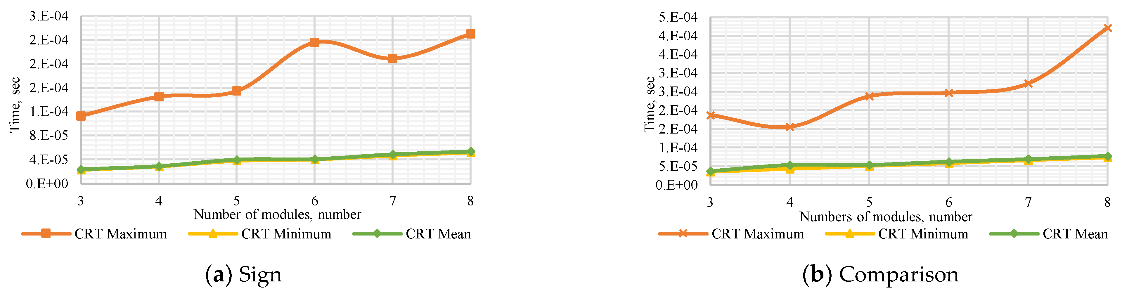
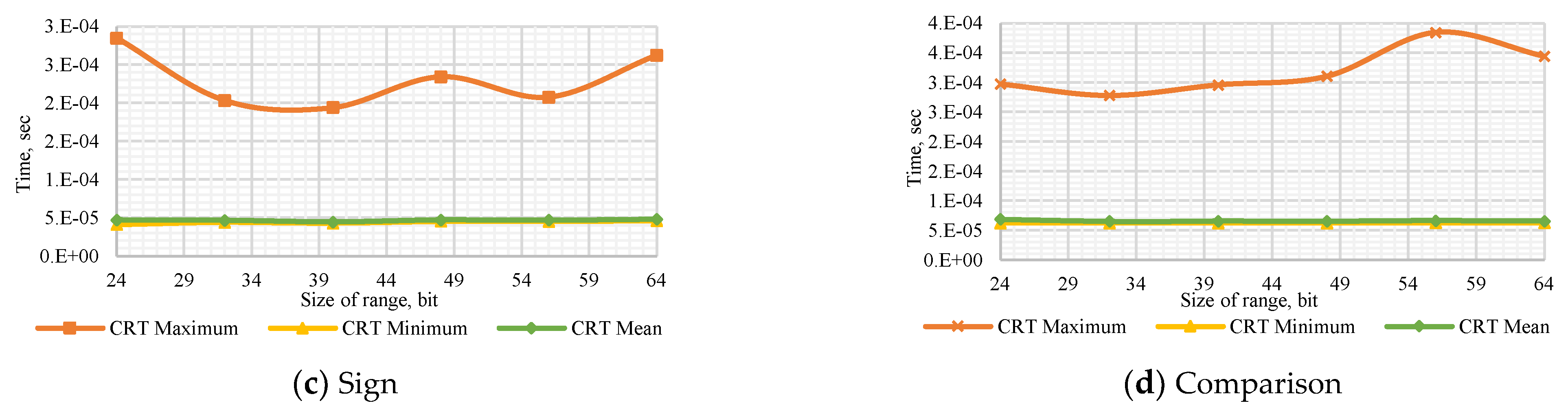
Figure A1.
Performance of CRT method to (a) determine the number’s sign with a dynamic number of modules , (b) compare dynamic numbers of modules , (c) determine the number’s sign with a dynamic bit width, and (d) compare numbers with dynamic bit width.
Figure A1.
Performance of CRT method to (a) determine the number’s sign with a dynamic number of modules , (b) compare dynamic numbers of modules , (c) determine the number’s sign with a dynamic bit width, and (d) compare numbers with dynamic bit width.
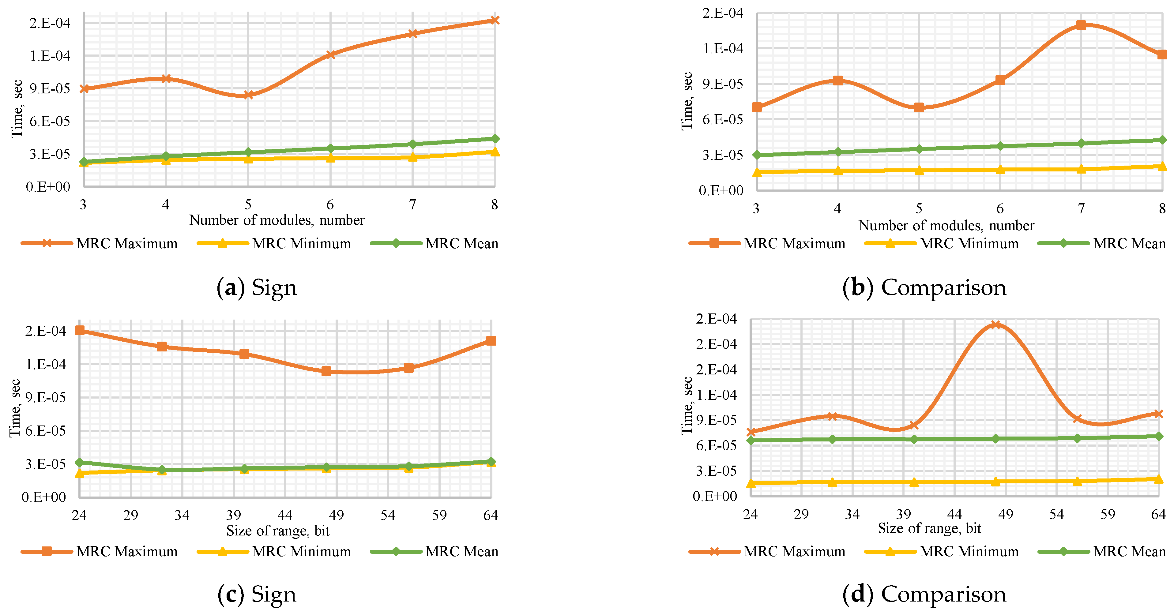
Figure A2.
Performance of MRC method to (a) determine the number’s sign with a dynamic number of modules , (b) compare dynamic number of modules , (c) determine the number’s sign with a dynamic bit width, and (d) compare numbers with dynamic bit width.
Figure A2.
Performance of MRC method to (a) determine the number’s sign with a dynamic number of modules , (b) compare dynamic number of modules , (c) determine the number’s sign with a dynamic bit width, and (d) compare numbers with dynamic bit width.
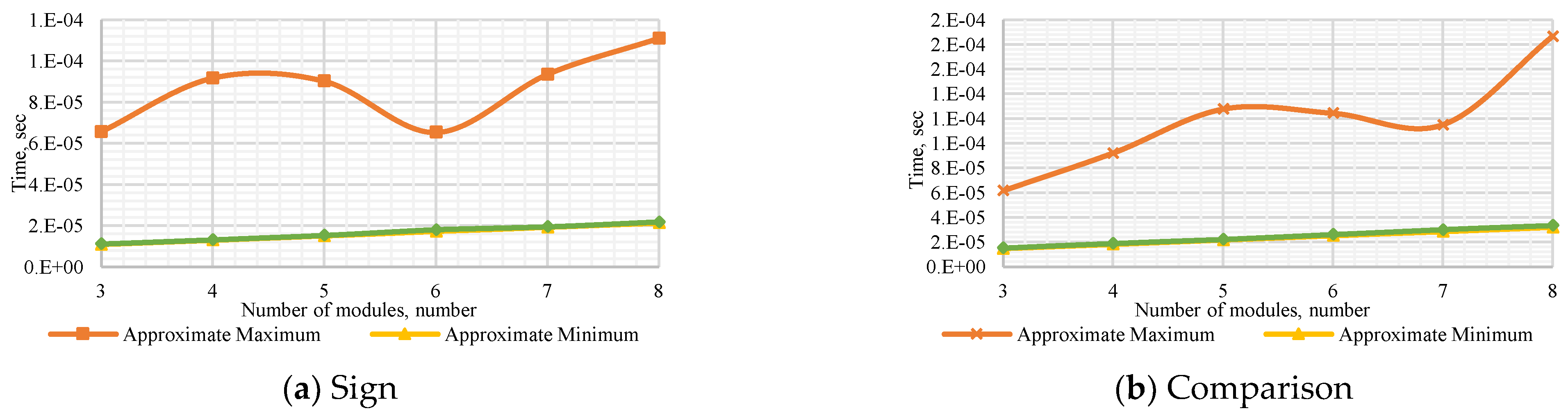
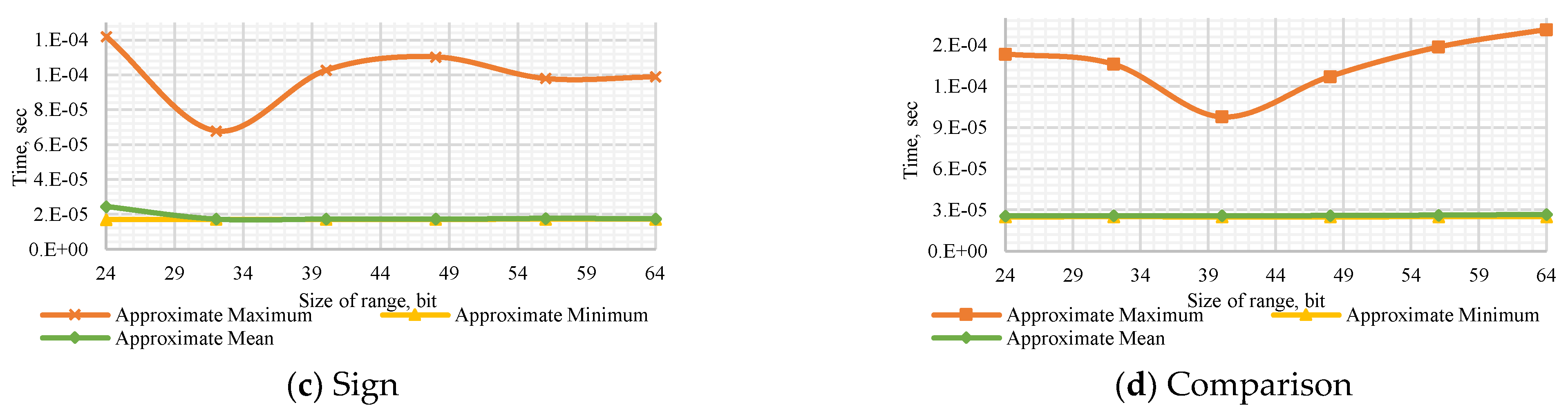
Figure A3.
Performance of the Approximate Method to (a) determine the number’s sign with a dynamic number of modules , (b) compare the dynamic number of modules , (c) determine the number’s sign with a dynamic bit width, and (d) compare numbers with dynamic bit width.
Figure A3.
Performance of the Approximate Method to (a) determine the number’s sign with a dynamic number of modules , (b) compare the dynamic number of modules , (c) determine the number’s sign with a dynamic bit width, and (d) compare numbers with dynamic bit width.
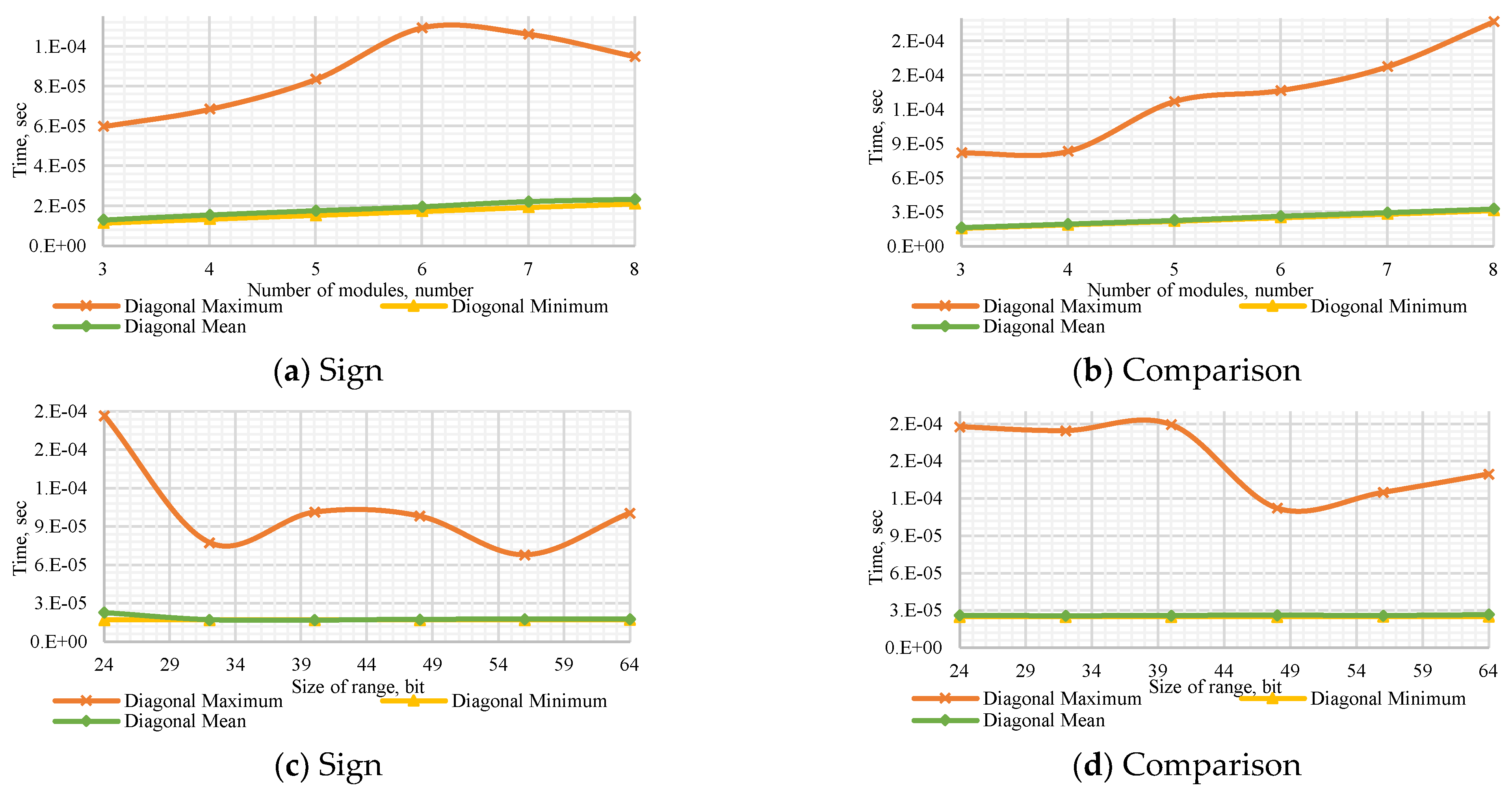
Figure A4.
Performance of the Diagonal Method to (a) determine the number’s sign with a dynamic number of modules , (b) compare dynamic numbers of modules , (c) determine the number’s sign with a dynamic bit width, and (d) compare numbers with dynamic bit width.
Figure A4.
Performance of the Diagonal Method to (a) determine the number’s sign with a dynamic number of modules , (b) compare dynamic numbers of modules , (c) determine the number’s sign with a dynamic bit width, and (d) compare numbers with dynamic bit width.
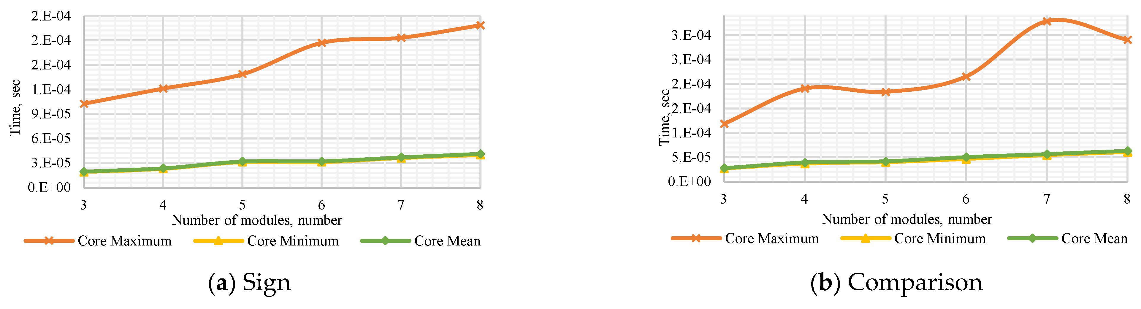
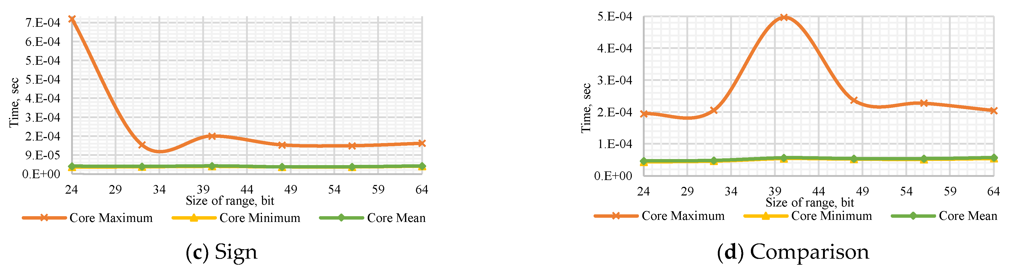
Figure A5.
Performance of the Core Method to (a) determine the number’s sign with a dynamic number of modules , (b) compare dynamic numbers of modules , (c) determine the number’s sign with a dynamic bit width, and (d) compare numbers with dynamic bit width.
Figure A5.
Performance of the Core Method to (a) determine the number’s sign with a dynamic number of modules , (b) compare dynamic numbers of modules , (c) determine the number’s sign with a dynamic bit width, and (d) compare numbers with dynamic bit width.
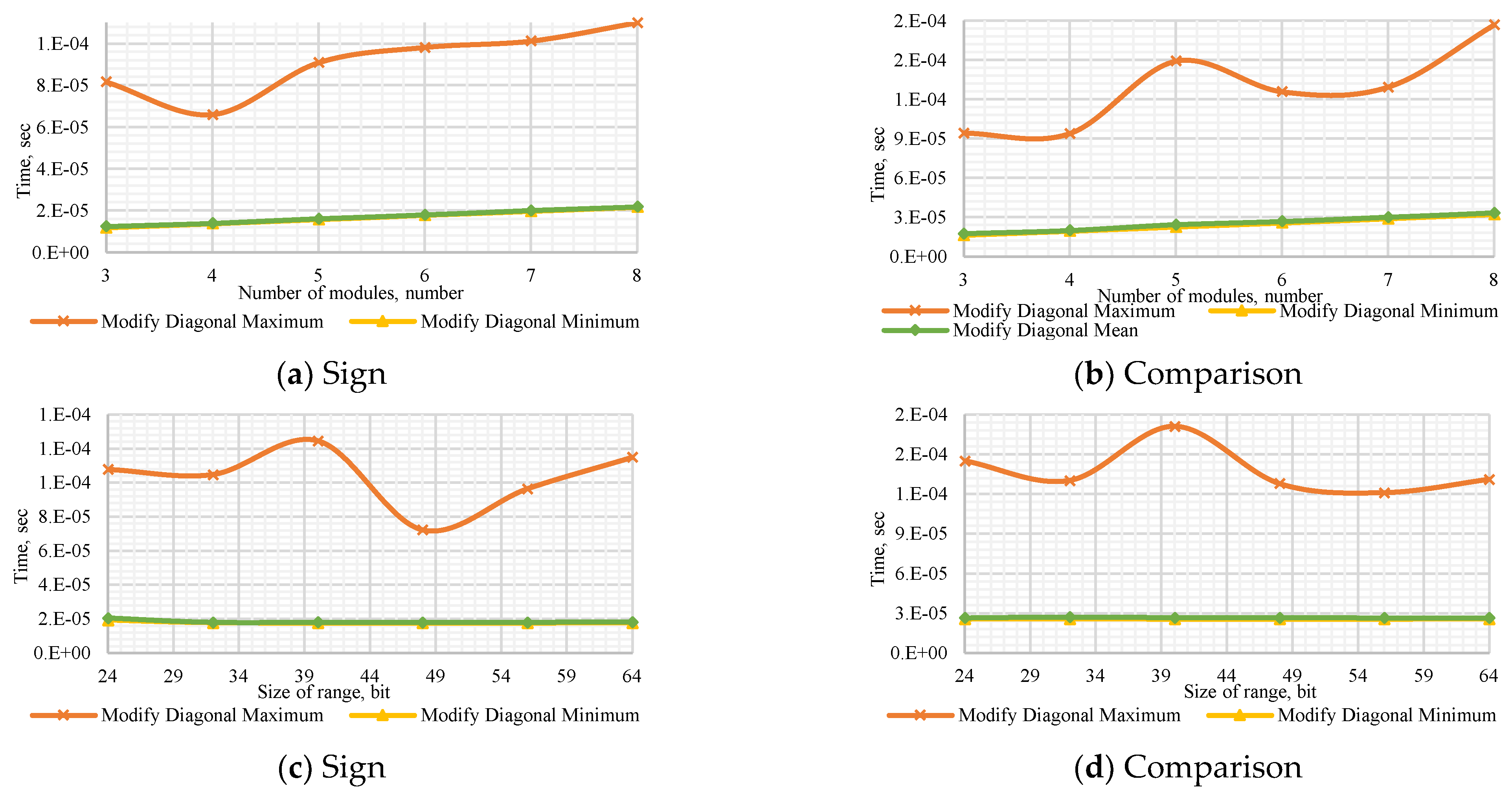
Figure A6.
Performance of the Modify Diagonal Method to (a) determine the number’s sign with a dynamic number of modules , (b) compare dynamic numbers of modules , (c) determine the number’s sign with a dynamic bit width, and (d) compare numbers with dynamic bit width.
Figure A6.
Performance of the Modify Diagonal Method to (a) determine the number’s sign with a dynamic number of modules , (b) compare dynamic numbers of modules , (c) determine the number’s sign with a dynamic bit width, and (d) compare numbers with dynamic bit width.
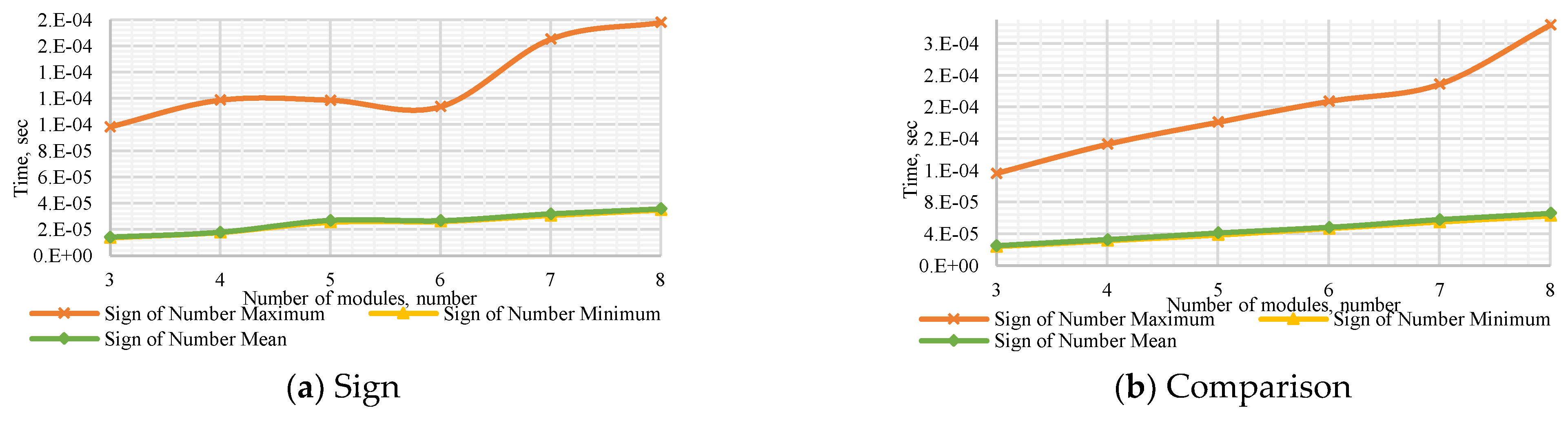
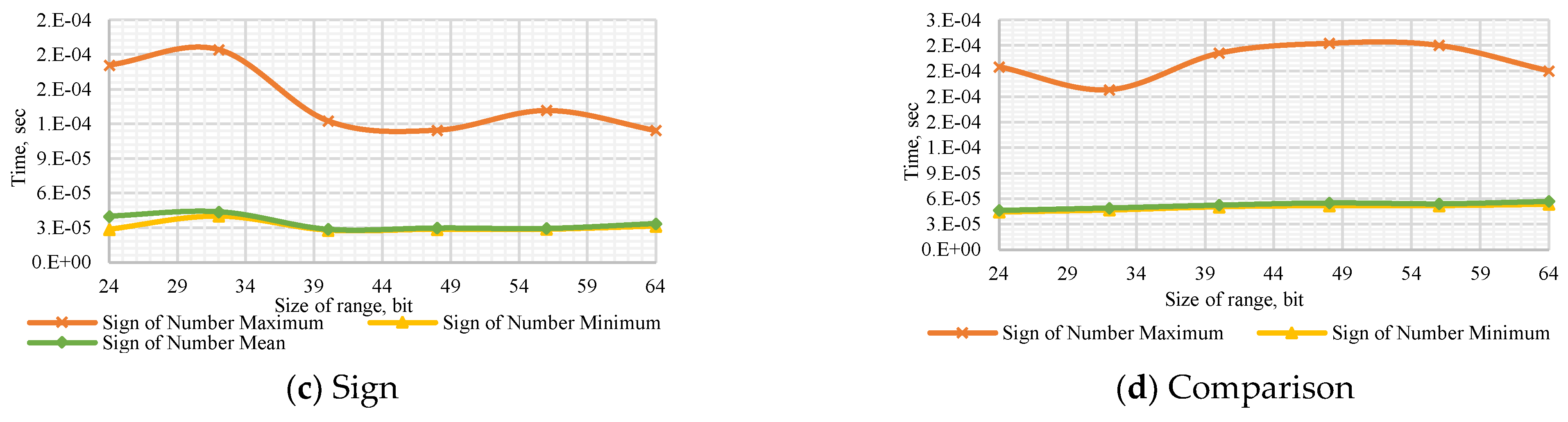
Figure A7.
Performance of the Sign of Number Method to (a) determine the number’s sign with a dynamic number of modules , (b) compare dynamic numbers of modules , (c) determine the number’s sign with a dynamic bit width, and (d) compare numbers with dynamic bit width.
Figure A7.
Performance of the Sign of Number Method to (a) determine the number’s sign with a dynamic number of modules , (b) compare dynamic numbers of modules , (c) determine the number’s sign with a dynamic bit width, and (d) compare numbers with dynamic bit width.
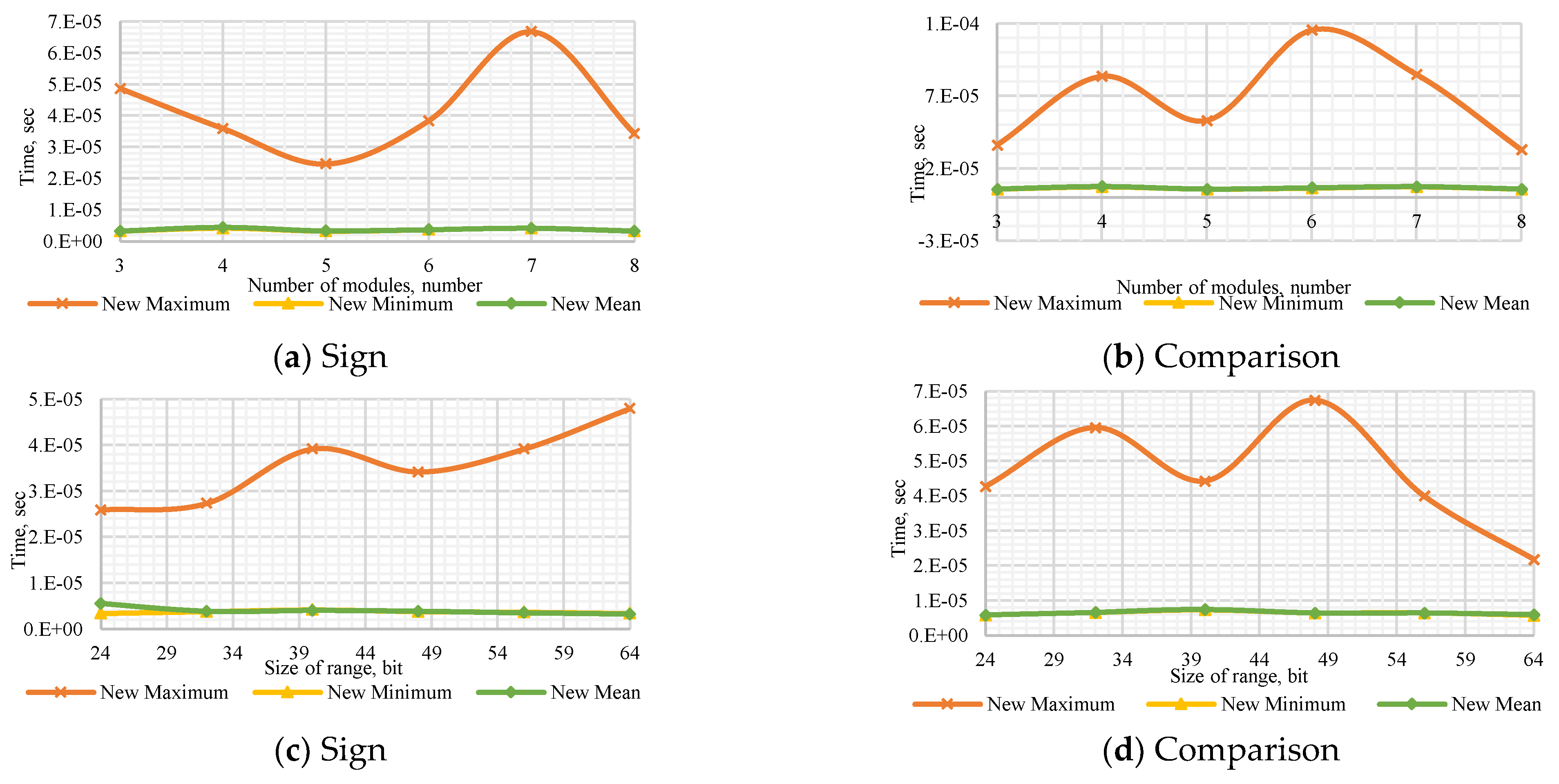
Figure A8.
Performance of the DSN-EN method to (a) determine the number’s sign with a dynamic number of modules , (b) compare dynamic numbers of modules , (c) determine the number’s sign with a dynamic bit width, and (d) compare numbers with dynamic bit width.
Figure A8.
Performance of the DSN-EN method to (a) determine the number’s sign with a dynamic number of modules , (b) compare dynamic numbers of modules , (c) determine the number’s sign with a dynamic bit width, and (d) compare numbers with dynamic bit width.
References
- Pirlo, G.; Impedovo, D. A new class of monotone functions of the residue number system. Int. J. Math. Models Methods Appl. Sci. 2013, 7, 803–809. [Google Scholar]
- Piestrak, S.J. A note on RNS architectures for the implementation of the diagonal function. Inf. Process. Lett. 2015, 115, 453–457. [Google Scholar] [CrossRef]
- Dimauro, G.; Impedovo, S.; Pirlo, G. A new technique for fast number comparison in the residue number system. IEEE Trans. Comput. 1993, 42, 608–612. [Google Scholar] [CrossRef]
- Babenko, M.; Deryabin, M.; Piestrak, S.; Patronik, P.; Chervyakov, N.; Tchernykh, A.; Avetisyan, A. RNS Number Comparator Based on a Modified Diagonal Function. Electronics 2020, 9, 1784. [Google Scholar] [CrossRef]
- Van Vu, T. Efficient implementations of the Chinese remainder theorem for sign detection and residue decoding. IEEE Trans. Comput. 1985, 100, 646–651. [Google Scholar] [CrossRef]
- Babenko, M.G.; Tchernykh, A.N.; Chervyakov, N.I.; Kuchukov, V.A.; Miranda-López, V.; Rivera-Rodriguez, R.; Du, Z. Efficient number comparison in the residue number system based on positional characteristics. Proc. Inst. Syst. Program. RAS 2019, 31, 187–202. [Google Scholar] [CrossRef]
- Babenko, M.; Piestrak, S.J.; Chervyakov, N.; Deryabin, M. The Study of Monotonic Core Functions and Their Use to Build RNS Number Comparators. Electronics 2021, 10, 1041. [Google Scholar] [CrossRef]
- Isupov, K.; Knyazkov, V.; Kuvaev, A. Design and implementation of multiple-precision BLAS Level 1 functions for graphics processing units. J. Parallel Distrib. Comput. 2020, 140, 25–36. [Google Scholar] [CrossRef]
- Isupov, K. Using Floating-Point Intervals for Non-Modular Computations in Residue Number System. IEEE Access 2020, 8, 58603–58619. [Google Scholar] [CrossRef]
- Gentry, C. A Fully Homomorphic Encryption Scheme; Stanford University: Stanford, CA, USA, 2009. [Google Scholar]
- Pulido-Gaytan, B.; Tchernykh, A.; Cortés-Mendoza, J.M.; Babenko, M.; Radchenko, G.; Avetisyan, A.; Drozdov, A.Y. Privacy-preserving neural networks with Homomorphic encryption: Challenges and opportunities. Peer-Peer Netw. Appl. 2021, 14, 1666–1691. [Google Scholar] [CrossRef]
- Cortés-Mendoza, J.M.; Tchernykh, A.; Babenko, M.; Pulido-Gaytán, L.B.; Radchenko, G.; Leprevost, F.; Wang, X.; Avetisyan, A. Privacy-preserving logistic regression as a cloud service based on residue number system. In Russian Supercomputing Days; Springer Cham: Berlin/Heidelberg, Germany, 2020. [Google Scholar]
- Kamara, S.; Kristin, L. Cryptographic Cloud Storage. In International Conference on Financial Cryptography and Data Security; Springer: Berlin/Heidelberg, Germany, 2010. [Google Scholar]
- Kucherov, N.; Kuchukova, E.; Tchernykh, A.; Kuchukov, V.; Babenko, M. Towards Optimizing Cloud Computing Using Residue Number System. J. Phys. Conf. Ser. 2021, 1715, 012052. [Google Scholar] [CrossRef]
- Babenko, M.; Tchernykh, A.; Golimblevskaia, E.; Pulido-Gaytan, L.B.; Avetisyan, A. Homomorphic Comparison Methods: Technologies, Challenges, and Opportunities. In Proceedings of the 2020 International Conference Engineering and Telecommunication (En&T), IEEE, Dolgoprudny, Russia, 25–26 November 2020. [Google Scholar]
- Babenko, M.; Tchernykh, A.; Pulido-Gaytan, B.; Golimblevskaia, E.; Cortés-Mendoza, J.M.; Avetisyan, A. Experimental Evaluation of Homomorphic Comparison Methods. In Proceedings of the 2020 Ivannikov Ispras Open Conference (ISPRAS), Moscow, Russia, 10–11 December 2020. [Google Scholar]
- Lee, Y.; Lee, J.-W.; Kim, Y.-S.; No, J.-S. Near-optimal polynomial for modulus reduction using l2-norm for approximate homomorphic encryption. IEEE Access 2020, 8, 144321–144330. [Google Scholar] [CrossRef]
- Chase, M.; Chen, H.; Ding, J.; Goldwasser, S.; Gorbunov, S.; Hoffstein, J.; Lauter, K.; Lokam, S.; Moody, D.; Morrison, T.; et al. Security of homomorphic encryption. HomomorphicEncryption. Org. Redmond WA. Tech. Rep. 2017. [Google Scholar]
- Shiryaev, E.; Golimblevskaia, E.; Babenko, M.; Tchernykh, A.; Pulido-Gaytan, B. Improvement of the Approximate Method for the Comparison Operation in the RNS. In Proceedings of the 2020 International Conference Engineering and Telecommunication (En&T), IEEE, Dolgoprudny, Russia, 25–26 November 2020. [Google Scholar]
- Babenko, M.; Tchernykh, A.; Chervyakov, N.; Kuchukov, V.; Miranda-López, V.; Rivera-Rodriguez, R.; Du, Z.; Talbi, E.-G. Positional Characteristics for Efficient Number Comparison over the Homomorphic Encryption. Program. Comput. Softw. 2019, 45, 532–543. [Google Scholar] [CrossRef]
- Pulido-Gaytan, L.B.; Tchernykh, A.; Cortés-Mendoza, J.M.; Babenko, M.; Radchenko, G. A Survey on Privacy-Preserving Machine Learning with Fully Homomorphic Encryption. In Communications in Computer and Information Science; Springer: Berlin/Heidelberg, Germany, 2021; pp. 115–129. [Google Scholar] [CrossRef]
- Garner, H.L. The residue number system. Presented at the Western Joint Computer Conference (IRE-AIEE-ACM ’59 (Western)), San Francisco, CA, USA, 3–5 March 1959. [Google Scholar] [CrossRef]
- Pei, D.; Arto, S.; Cunsheng, D. Chinese Remainder Theorem: Applications in Computing, Coding, Cryptography; World Scientific: Singapore, 1996. [Google Scholar]
- Yassine, H.M.; Moore, W.R. Improved mixed-radix conversion for residue number system architectures. IEE Proc. G Circuits Devices Syst. 1991, 138, 120–124. [Google Scholar] [CrossRef]
- Chervyakov, N.I.; Molahosseini, A.S.; Lyakhov, P.A.; Babenko, M.G.; Deryabin, M.A. Residue-to-binary conversion for general moduli sets based on approximate Chinese remainder theorem. Int. J. Comput. Math. 2016, 94, 1833–1849. [Google Scholar] [CrossRef]
- Burgess, N. Scaled and unscaled residue number system to binary conversion techniques using the core function. In Proceedings of the 13th IEEE Sympsoium on Computer Arithmetic, Asilomar, CA, USA, 6–9 July 1997. [Google Scholar]
- Miller, D.D.; Altschul, R.E.; King, J.R.; Polky, J.N. Analysis of the Residue Class Core Function of Akushskii, Burcev, and Pak. In Residue Number System Arithmetic: Modern Applications in Digital Signal Processing; IEEE Publications: Manhattan, NY, USA, 1986; pp. 390–401. [Google Scholar]
- Gonnella, J. The application of core functions to residue number systems. IEEE Trans. Signal Processing 1991, 39, 69–75. [Google Scholar] [CrossRef]
- Chervyakov, N.I.; Babenko, M.G.; Deryabin, M.A.; Nazarov, A.S.; Shabalina, M.N. Computation of Positional Characteristics of Numbers in RNS Based on Approximate Method. In Proceedings of the 2016 IEEE NW Russia Young Researchers in Electrical and Electronic Engineering Conference (EIConRusNW), St. Petersburg, Russia, 2–3 February 2016. [Google Scholar]
| Publisher’s Note: MDPI stays neutral with regard to jurisdictional claims in published maps and institutional affiliations. |
© 2022 by the authors. Licensee MDPI, Basel, Switzerland. This article is an open access article distributed under the terms and conditions of the Creative Commons Attribution (CC BY) license (https://creativecommons.org/licenses/by/4.0/).


 ,
, 


