Abstract
The spatiotemporal model consists of stationary and non-stationary data, respectively known as the Generalized Space–Time Autoregressive (GSTAR) model and the Generalized Space–Time Autoregressive Integrated (GSTARI) model. The application of this model in forecasting climate with rainfall variables is also influenced by exogenous variables such as humidity, and often the assumption of error is not constant. Therefore, this study aims to design a spatiotemporal model with the addition of exogenous variables and to overcome the non-constant error variance. The proposed model is named GSTARI-X-ARCH. The model is used to predict climate phenomena in West Java, obtained from National Aeronautics and Space Administration Prediction of Worldwide Energy Resources (NASA POWER) data. Climate data are big data, so we used knowledge discovery in databases (KDD) in this study. The pre-processing step is collecting and cleaning data. Then, the data mining process with the GSTARI-X-ARCH model follows the Box–Jenkins procedure: model identification, parameter estimation, and diagnostic checking. Finally, the post-processing step for visualization and interpretation of forecast results was conducted. This research is expected to contribute to developing the spatiotemporal model and forecast results as recommendations to the relevant agencies.
MSC:
62M10; 62H11
1. Introduction and Background
Climate change is a world problem that is very crucial for immediate preventive action []. The causes of climate change are complex and controversial natural, anthropogenic processes with global and local effects. Climate occurs over a long period regionally and globally. The elements of climate include air temperature, rainfall, air pressure, wind direction, humidity, and other climate elements []. Climate significantly impacts the socioeconomic field, directly and indirectly affecting sectors of human life. The awareness of community response is still deficient in mitigating and adapting to the severe challenges of climate change []. A significant influence also affects the agricultural sector. Due to the drought and rainy season, farmers changed irrigation techniques and harvest times []. The soil surface temperature’s climatic elements also affect the city’s development [,]. One of the climate impacts that have a significant impact is La Niña which causes an increase in rainfall in the Western Pacific region [,,]. In West Java, La Niña generally causes temporal changes in the volume and pattern of rainfall []. Rainfall is divided into wet months in December, January, and February (DJF) and dry months in June, July, and August (JJA). Rainfall is also influenced by other climatic elements, namely humidity, so statistical analysis is needed to predict rainfall in an area. The relationship between rainfall and humidity usually lasts for a long time, such as months or years.
Climate data that are sorted by time are called time series data. Time series models are divided into univariate and multivariate based on the number of variables [,]. In [], the model is divided into stationary and non-stationary. The study also identified the procedures for modeling the Box–Jenkins-based time series, which include the identification process, parameter estimation, and diagnostic checking []. The model identification stage is conducted by testing the stationary and determining the order of the model. Next, parameter estimation is carried out to obtain the forecast value. Diagnostic checking tests the model’s assumptions of normal multivariate, white noise, and homoscedasticity.
Climate data sorted by a combination of time and location simultaneously are known as spatiotemporal data, which include the Space–Time Autoregressive (STAR) [,] and the GSTAR models []. In [], the STAR model is used on stationary data to analyze the crime rate in the city of Boston. The STAR model has the assumption that each location has homogeneous characteristics. Meanwhile, the STAR model is weak because it is only applicable to homogeneous locations. The model development was carried out by assuming heterogeneous locations for the GSTAR model on stationary data and the GSTARI model on non-stationary data. In [], the GSTAR model is used to forecast oil production at the Jatibarang field well using the ordinary least squares (OLS) method, assuming that the error variance is constant [].
The GSTAR model is developed by estimating parameters using the autoregressive conditional heteroscedasticity (ARCH) model. The GSTAR-ARCH model is built for stationary data and the GSTARI-ARCH model is for non-stationary data [,,,]. The GSTAR-ARCH model is applied in forecasting inflation data in West Java [] and the GSTARI-ARCH model is used to forecast the CPI data in North Sumatra []. In addition, the GSTAR–seemingly unrelated regressions (SUR) model is developed to overcome autocorrelation errors for predicting rainfall in Batu City, Malang []. In [,,,], the GSTAR model is developed into a Generalized Space–Time Autoregressive Integrated Moving Average (GSTARIMA) with non-stationary data used for economic analysis.
The GSTAR/GSTARI model is developed by adding exogenous variables that affect the response variables. These models are called the Generalized Space–Time Autoregressive—Exogenous (GSTAR-X) and the Generalized Space–Time Autoregressive Integrated—Exogenous (GSTARI-X) [,,,]. Elfiyan et al. [] developed the GSTARI-X model on non-stationary data with parameter estimation using ordinary least squares (OLS). This model predicts the number of active family planning participants in West Java as a response variable and the number of field family planning managers as an exogenous variable. Suhartono et al. [] further developed the GSTARX model with generalized least squares (GLS) known as the GSTARX-GLS model. The GSTARX-GLS model is applied to forecast inflation in four major Indonesian cities. The response variables are the increase in fuel prices and the exogenous variables are the Eid al-Fitr holiday calendar. Ashari et al. [] modified the GSTARX into GSTARX-SUR model using the SUR method by adding exogenous variables and parameter estimation to overcome autocorrelated errors. The GSTARX-SUR model is applied to predict black cocoa pod attack (response variable) and rainfall (exogenous variable).
Based on the literature review, the gap in previous research in the GSTARX and GSTARIX models [,] cannot solve the problem of non-constant error variance. In applying the spatiotemporal model, this often happens in forecasting. Then, the GSTAR-ARCH and GSTARI-ARCH models [,] do not contain exogenous variables. In forecasting phenomena, especially climate, the response variable is influenced by exogenous variables. In addition, the data used in previous research are small (1 MB–20 MB). The climate data on the NASA POWER website are big data. The NASA POWER data consist of 100 variables with three subclasses from all locations worldwide. So, the KDD process in data mining methodology is needed in processing climate data. Several previous researchers have used the KDD process. Abdullah [] forecasted the education quality in Indonesia using a data mining approach through the SAR–Kriging model. The model used is only based on location and involves time, even though phenomena that occur daily can also be sorted by time. Then, Munandar et al. [] used a data mining approach to climate data with the PCA-VARI model. The PCA-VARI model does not involve the assumption of location heterogeneity like the GSTAR/GSTARI model. Next, Monika et al. [] forecast rainfall in Bandung using the ARIMA-ARCH model, a univariate time-series model.
Based on the explanation above, in this research, we contribute to building a spatiotemporal model with simultaneous assumptions, including non-stationary data, adding exogenous variables, overcoming non-constant error variances, and the KDD process approach. The proposed model is called the GSTARI-X-ARCH model, which overcomes the gap of previous research. The GSTARI-X-ARCH model is used for forecasting climate phenomena in West Java with rainfall and humidity as the response and exogenous variables, respectively. Theoretical studies and applications in this current study are supported by computing with open-source R software. The obtained results are expected to contribute to scientific development regarding stochastic modeling in spatiotemporal analysis. Also, quantitative results from forecasting climate phenomena in West Java are expected to be useful for the relevant agencies as an early warning.
2. Materials and Methods
2.1. Non-Stationary Univariate Time Series Analysis
A consecutive observational sequence of a phenomenon with an identical time interval is called a time series []. Continuous time series are observations made continuously, whereas discrete time series are observations made at certain time intervals []. The time series analysis based on stationary data is divided into stationary and non-stationary. Meanwhile, it is categorized as univariate and multivariate regarding the number of variables.
The stochastic process is a sequence of random variables , with sample space and time index. For example, given a set of random variables , the time series is a stochastic process where is a random variable with time index in the sample space []. The data are stationary when there is no significant change. For example, a stochastic process of order th is considered stationary when for all , integers, and is a one-dimensional distribution function. Stationary testing is performed using the augmented Dicky–Fuller (ADF) test, which is expressed as follows [,]:
where
: time series data at time
: time series data at time
: parameter, if , so there is a unit root
: error at time
The ADF test results on non-stationary data are obtainable through a differencing process, which is a method for stabilizing non-stationary data by reducing the observation value from the previous one . The differencing process on the -order, where represents the backshift operator is stated as follows [,]:
The autoregressive integrated (ARI) model is a non-stationary univariate time series. The ARI model is expressed below, where represents autoregressive order, represents observation at time with first order differencing, represent autoregressive parameter on time order , and differencing order with assumptions [,]:
2.2. Distance Inverse Weight Matrix
The weight matrix is a square matrix with elements of the corresponding location weights. The weight matrix obtained by calculating the actual distance among locations is called the inverse distance weight matrix. The distance inverse weight calculation is as follows []:
where is the inverse weight matrix element of the distance at locations and , and represents the distance from location to location .
2.3. Spatiotemporal Model Based on Box–Jenkins Method
The spatiotemporal model was first developed in 1980 by Pfeifer and Deutch [,]. The GSTAR model assumes heterogeneous location characteristics and it is expressed in terms of matrix as follows [,]:
where
: observation vector at time
: observation vector at time
: spatial order at the -th autoregressive
: autoregressive and space–time parameters on time order and spatial order
: weight matrix on the spatial order
: error vector at time , assuming
The GSTARI is a development of the GSTAR model on non-stationary data. The general form of the GSTARI model is written as follows []:
where .
The development of the GSTARI model with the addition of exogenous variables is known as the GSTARI-X. The GSTARI-X model in the form of matrix notation is expressed as follows [,]:
where and represents sequentially exogenous parameters and observations of exogenous variables, respectively. The GSTARI-X model assumes zero mean error and constant variance.
2.4. Space–Time Autoregressive Autocorrelation Function (STACF) and Space–Time Partial Autocorrelation Function (STPACF)
STACF and STPACF plots can be used in identification process of Spatio-Temporal model [,]. The STACF was obtained by standardizing the autocovariance function of the time lag m for observations with the -th and -th spatial lag, . According to [], the STACF generally has a constant variance for each spatial lag, defined as follows []:
To identify the spatiotemporal model sequence, the truncated lag in the STPACF plot needs to be examined. STPACF for spatial order in the Yule–Walker equation is the last coefficient of and as shown in Appendix A.
2.5. Autoregressive Conditional Heteroscedasticity (ARCH) Model
The GSTARI-X error assumption with non-constant variance is examined through the ARCH, a time series model for modeling the heteroscedasticity of variance based on previous data [,]. The error variance equation for the ARCH model (1) is expressed in Equation (9) [,]:
From Equation (9), it was observed that the error variance has two components, namely the constant and the square of the previous period error . Conditional heteroscedasticity is the error model , having non-constant properties and is based on the last error value . The ARCH (p) model is expressed below [,]:
where
: conditional variance at time
: intercept or constant error
: parameter ARCH model
dan
2.6. The Development of the GSTARI-X-ARCH Model
The GSTARI-X-ARCH model is an extension of the GSTARI-X model in Equation (7) with error estimation through the ARCH model in Equation (9). Furthermore, the GSTARI-X-ARCH model was developed to forecast spatiotemporal data with non-constant error variances, non-stationary data, and exogenous variables. The general form of the GSTARI-X -ARCH (q) model is stated as follows:
where
represents the set of information available up to time , represents conditional variance, represents the conditional variance diagonal matrix, denotes the conditional variance matrix, and is the standardization error vector. Forecasting procedures with the GSTARI-X-ARCH model and parameter estimation are presented in Figure 1.
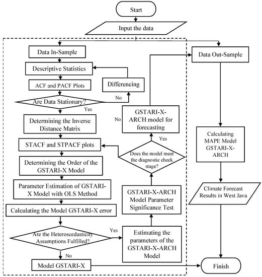
Figure 1.
GSTARI-X-ARCH model procedure.
2.7. Diagnostic Checking
Diagnostic checks are performed to observe whether the error assumptions in the model have been met or not. Generally, three error assumptions have to be met, namely the multivariate properties of white noise, multivariate normal distribution, and homoscedasticity. The Portmanteau test used to check the error assumption is multivariate white noise [,], which is a sequence of random variables with mean 0 and constant variance . Chi-Squared QQ plots obtained from the value of which represents the test statistic were used to check the assumption of multivariate normal error distribution []. The Lagrange multiplier (LM) test for the assumption of homoscedasticity is expressed in [,,]:
where is the observation numbers, represents the determination coefficient of the regression model.
2.8. Mean Absolute Percentage Error (MAPE)
Forecasting accuracy was obtained by calculating the MAPE value, the average percent of absolute error value, and the actual value in each period. The MAPE formula for the spatiotemporal model is expressed below []:
where and represent the actual and error values, respectively, whereas and denote the numbers of time series observation and location observation, respectively.
2.9. Knowledge Discovery in Database (KDD) Data Mining
Big data is a massive and complex dataset, which makes it difficult to be processed with simple data warehouse tools []. Examples of big data in daily life are the huge data quantities regularly obtained from climate observations [,], Twitter user data [], banking transaction data, and others. Analyzing these saved data is a crucial activity as the human ability to individually record the evaluated data patterns is very limited. Therefore, data mining is needed to support human work in learning and informing data. Data mining is used to extract useful information and detect patterns from data, often large data sets closely related to knowledge discovery in databases and data science []. This is because it is a technique that functions descriptively and predictively in big data when searching for essential information and trending patterns [,]. Alternative names for data mining are knowledge discovery (mining) in databases (KDD), knowledge extraction, data/pattern analysis, data archeology, data dredging, information harvesting, business intelligence, and others. Those factors encouraging data mining development are scalability, high dimensionality, heterogeneous/complex data, data ownership, and non-traditional analysis []. The KDD data mining method consists of three stages, namely pre-processing, data mining process, and post-processing, and its procedure is shown in Figure 2 [,].
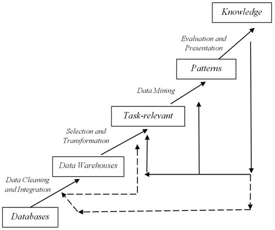
Figure 2.
KDD procedure in data mining.
3. Results
This section describes the implementation of the GSTARI-X-ARCH model using KDD data mining. The KDD process is needed in this study as a function of the description and forecasting of NASA POWER climate data which are big data. The stages of the KDD process are explained as follows:
3.1. Pre-Processing Step
The description of the data used in the GSTARI-ARCH model simulation is as follows:
- The source of data comes from NASA POWER. It can be accessed via https://power.larc.nasa.gov/data-access-viewer/ (accessed on 25 May 2022). Furthermore, we can obtain information of the data storage size from the website https://disc.gsfc.nasa.gov/ (accessed on 25 May 2022). The data storage size is 3,370,469 TB with 100 variables. Climate data with rainfall and humidity parameters in the West Java region, consisting of 27 regencies/cities, are calculated from December 1989 to 2021 with daily time intervals. Meanwhile, each location’s latitude and longitude coordinate data were obtained from https://www.latlong.net/ (accessed on 25 May 2022).
- The data cleaning process is the preliminary stage when forecasting climate phenomena using the GSTARI-X-ARCH model with a data mining approach. Daily climate data for 27 districts and cities in West Java consists of 11,719 data. The rainfall is a response variable, and humidity is an exogenous variable. Then, the daily data are aggregated into monthly data using R software. The data aggregate process resulted in 385 monthly data for each location. In this study, the data selection process is conducted by selecting rainfall data that occur in the wet months, namely December, January, and February (DJF). At this stage, it produces 97 data for each location. Figure 3 shows the brief pre-processing steps with the selected places representing the same observation value of 11 locations as input in the data mining process.
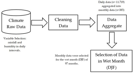 Figure 3. Pre-processing step.
3.2. Data Mining Process
We divided the pre-processed data () into two parts, namely 87 (in-sample) and 10 (out-sample). The model identification stage tests the stationary data of rainfall and humidity using the augmented Dickey–Fuller (ADF) test. Table 1 shows that rainfall data in 10 locations, including Bandung, Bekasi, Bogor, Cirebon, Sukabumi, Tasikmalaya, Majalengka, Purwakarta, and Kuningan, have a -value above the critical value . When the -value is more significant than 0.05, is rejected, meaning the data are not stationary. In Pangandaran, rainfall data have a smaller -value compared to the critical value of , hence, is not rejected, indicating that data are stationary. We performed the differencing for non-stationary rainfall data and obtained a -value smaller than . The ADF test on humidity data has shown stationary data results. is not rejected when the -value is less than , so the humidity data do not require a differencing process.

Table 1.
Stationary assumption checked by using ADF test.
We determine the order of the model using the STACF and STPACF plots. Figure 4 shows that spatial lag 0 is cut off at lags 1,2,3,4,5, and 10. In spatial lag 1, STPACF is cut off at lags 1,3,4,5,6, and 10. In this case, we used the parsimony principle to determine the order of the model. We choose spatial lag 0 and 1, which are cut off at time lag 1, so the model formed is GSTARI−X(1,1,1)−ARCH(1).
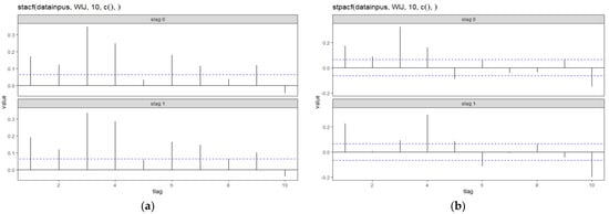
Figure 4.
STACF (a) and STPACF (b) diagrams.
Parameter estimation model GSTARI−X(1,1,1)−ARCH(1) requires an inverse distance weight matrix. We calculated an inverse distance weight using the actual distance from each location. The results of the calculation of the inverse distance weight matrix following Equation (11) are as follows:
We estimate the parameters of the GSTARI−X(1,1,1)−ARCH(1) model using the maximum likelihood method and the generalized least square (GLS) method. Table 2 shows the results of the estimated parameter model.
Table 2.
The result of the GSTARI−X(1,1,1)−ARCH(1) model parameter estimation.
The parameter estimation results and the inverse distance weight matrix are presented in matrix form following Equation (13). The GSTARI−X(1,1,1)−ARCH(1) model equation for each location is presented in Appendix B. We simultaneously tested the significance of the parameters, which showed -value = 2.2 × 10⁻¹⁶ (critical value). So, the parameters are significant in the model simultaneously.
In the next step, we perform a diagnostic check for the assumptions on model GSTARI−X(1,1,1)−ARCH(1). Test the homoscedasticity assumption to find out the model’s error variance. We use the LM test to determine the effect of ARCH on model error. The test results obtained a -value , which means that is not rejected. So, the error from the GSTARI−X(1,1,1)−ARCH(1) model has no ARCH error effect, which means the model satisfies the assumption of homoscedasticity. Then, we tested the white noise assumption to determine whether the GSTARI−X(1,1,1)−ARCH(1) model errors are uncorrelated. Table 3 shows the results of testing the white noise assumption using the Portmanteau test. The results of the Portmanteau test show that the -value is greater than the value or each time lag. is rejected so that the GSTARI−X(1,1,1)−ARCH(1) model satisfies the white noise assumption.
Table 3.
White noise assumption test results.
The last step in diagnostic checking was the normal multivariate assumption test using the QQ plot and visual histogram. It was observed from Figure 5 that the GSTARI−X(1,1,1)−ARCH(1) model errors are almost all close to the normal line. The GSTARI−X(1,1,1)−ARCH(1) model satisfies the multivariate normality assumption.
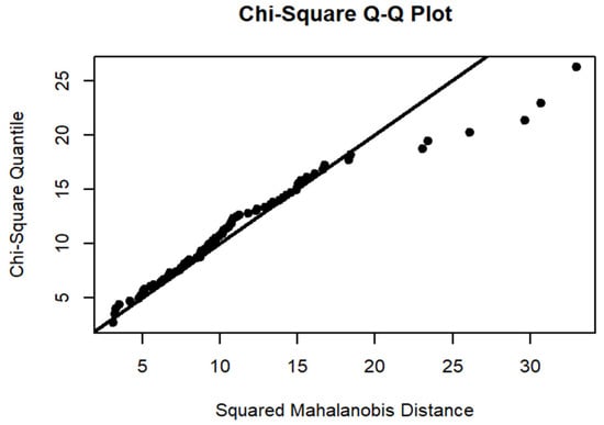
Figure 5.
QQ Plot.
After all the model assumptions were satisfied, the GSTARI−X(1,1,1)−ARCH(1) model became relevant for forecasting climate phenomena especially for rainfall in West Java. The GSTARI−X(1,1,1)−ARCH(1) model equation is applied to in-sample and out-sample data. The model’s accuracy is calculated using the mean absolute percentage error (MAPE) in Equation (12). Figure 6 shows the GSTARI−X(1,1,1)−ARCH(1) model results for in-sample data with a black line graph denoting the actual data and a red dot line graph representing the forecast data.
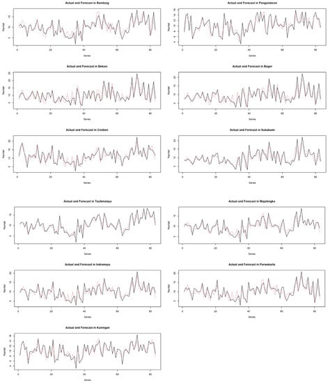
Figure 6.
Actual and forecast plots of climate phenomena at 11 locations in West Java.
Figure 6 represents the forecasting results of the GSTARI−X(1,1,1)−ARCH(1) model, showing almost the same trend pattern for each location. Specifically, results for the in-sample data have a MAPE value of 20%, whereas that of the out-sample was 19%, meaning that the forecast was accurate.
3.3. Post-Processing Step
The results of forecasting climate phenomena in West Java with the GSTARI−X(1,1,1)−ARCH(1) model were shown visually with a rainfall map created using the quantum geographic information systems (QGIS) program. The QGIS is open-source software used to manage spatial data. Figure 6 shows the rainfall forecast map for each month using the GSTARI−X(1,1,1)−ARCH(1) model.
Figure 7 represents the results of the visualization of rainfall forecasting in West Java. The map is presented with four color clusters, red, yellow, green, and blue, representing the intensity of rainfall in each area.
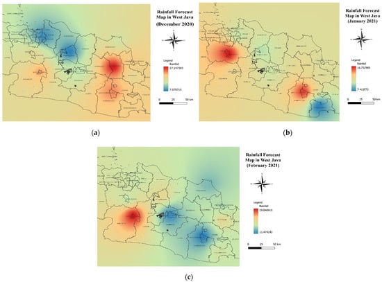
Figure 7.
Rainfall forecast map in West Java for December 2020 (a), January 2021 (b), and February 2021 (c).
4. Discussion
The data stored on the NASA website are very large, namely 3,370,469 TB, with 100 variables divided into three subclasses. The procedure for forecasting rainfall in West Java using the GSTARI-X-ARCH model with a data mining approach is carried out with the RStudio software. The built R script is used for data aggregation, data cleaning, parameter estimation, and diagnostic checking. The time required to execute the script is very fast (1 min–3 min). The first step is pre-processing; the NASA POWER climate and location coordinate data were collected through the selection process and cleaning. The pre-processed data were employed as input in the data mining process stage with the GSTARI-X-ARCH model through the Box–Jenkins method. The result of performing identification, parameter estimation, and diagnostic examination when forecasting climate phenomena showed an accurate forecast, which was visualized at the post-processing stage using QGIS in Figure 7, displaying rainfall intensity at each observation location. Figure 7a shows a map of the rainfall forecast for December 2020 in West Java. Based on the visualization results of the map, Majalengka Regency has high monthly rainfall intensity with an average value of 17.14 mm. The observation locations with low rainfall intensity are Purwakarta Regency and Bekasi city, having monthly average values of 7.07 mm and 7.47 mm, respectively. It was also observed that Tasikmalaya city and Bogor Regency had high rainfall intensities of 16.05 mm and 16.75 mm, respectively, in January 2021 based on the map visualization results shown in Figure 7b. The location with the lowest average monthly rainfall was Pangandaran Regency, at 7.41 mm. Specifically, Pangandaran Regency had low rainfall intensity in January 2021. According to Figure 7c, Sukabumi city had high rainfall intensity in February 2021, with an average of 19.04 mm. In this case, locations with low rainfall intensity include Bandung and Tasikmalaya cities, with average monthly rainfall values of 11.70 mm and 11.47 mm, respectively.
Based on the results processing data, the GSTARI-X-ARCH model proposed in this study can improve the models carried out in previous studies. In the forecasting procedure, the GSTARI-X-ARCH model implemented with the KDD process is better than the GSTARI-X [] and GSTARI-ARCH models [] because it can overcome the problem of non-constant error variance and the addition of exogenous variables. Furthermore, applying GSTARI-X-ARCH to forecast the climate data has a 19% MAPE value. It has a minimum MAPE value compared with the GSTARI-X model (20%) and the GSTARI-ARCH model (32%). From the comparison MAPE value, the GSTARI-X-ARCH model has a high accuracy for forecasting the future at a specific location with influence by surrounding locations.
5. Conclusions
This research develops a spatiotemporal model, namely the GSTARI-X-ARCH model. This model can overcome the gaps in the GSTARI-X and GSTARI-ARCH models in previous studies. In this study, the GSTARI-X-ARCH model with the KDD data mining approach has simultaneous assumptions such as adding exogenous variables, overcoming non-constant error variances, non-stationary data, and the KDD data mining process on big data.
This study uses the GSTARI-X-ARCH model to forecast climate phenomena in West Java. The procedure for applying the GSTARI-X-ARCH model with the KDD data mining approach is pre-processing, data mining process, and post-processing. The pre-processing is the first stage in modeling GSTARI-X-ARCH with a data mining approach. This stage begins by collecting time series data on climate phenomena in West Java with rainfall and humidity variables. Next, we cleaned the data by checking for missing values, aggregating the data monthly, and calculating descriptive statistics for the data. Then, the data mining process uses the GSTARI-X-ARCH model, which begins with model identification through data stationarity tests and ACF PACF plots. In this study, we use an inverse distance weight matrix using the distance between locations. Next, we calculate the parameter estimation using the OLS method and the GSTARI-X model error. For the error of the GSTARI-X model that satisfies the assumption of heteroscedasticity, we use the ARCH model for parameter estimation. So, it became the GSTARI-X-ARCH model. Next, diagnostic tests and climate forecasting with the GSTARI-X-ARCH model were conducted. Post-processing is the final stage for visualizing and interpreting the results of the rainfall forecast using the GSTARI-X-ARCH model.
The model implementation result shows that the GSTARI-X-ARCH model in forecasting climate phenomena has a high accuracy level with a MAPE value of 19%. The GSTARI-X-ARCH model improves the models proposed by previous researchers, namely the GSTARI-X and GSTARI-ARCH models. The GSTARI-X and GSTARI-ARCH models obtained higher MAPE values than the GSTARI-X-ARCH model. It shows that the accuracy of the GSTARI-X and GSTARI-ARCH models is lower.
This study helps predict the spatiotemporal phenomenon and the results are helpful for relevant agencies in making climate-related policies, especially regarding rainfall in West Java. Further research can be developed by adding the Kriging method for forecasting at unsampled locations, called the GSTARI-X-ARCH-Kriging model.
Author Contributions
Conceptualization, P.M. and B.N.R.; methodology, P.M.; software, P.M. and A.S.A.; validation, P.M., B.N.R. and A.S.A.; formal analysis, B.N.R.; investigation, A.S.A.; resources, B.N.R.; data curation, P.M.; writing—original draft preparation, P.M.; writing—review and editing, B.N.R. and A.S.A.; visualization, P.M. and A.S.A.; supervision, B.N.R.; project administration, P.M. and B.N.R.; funding acquisition, B.N.R. All authors have read and agreed to the published version of the manuscript.
Funding
This study was funded by the Padjadjaran Excellence Fastrack Scholarship (BUPP) and Academic Leadership Grant (ALG), grant number 2203/UN6.3.1/PT.00/2022.
Data Availability Statement
Not applicable.
Acknowledgments
The authors are grateful to Rector, Directorate of Research and Community Service (DRPM) and Studies Center of Modelling and Computation Faculty of Mathematics and Natural Sciences, Universitas Padjadjaran. The authors are also thanks to the collaborators in the RISE_SMA project 2022.
Conflicts of Interest
The authors declare no conflict of interest.
Appendix A
Appendix B
- GSTARI-X(1,1,1)-ARCH(1) model to forecast climate phenomena in Bandung
- GSTARI-X(1,1,1)-ARCH(1) model to forecast climate phenomena in Pangandaran
- GSTARI-X(1,1,1)-ARCH(1) model to forecast climate phenomena in Bekasi
- GSTARI-X(1,1,1)-ARCH(1) model to forecast climate phenomena in Bogor
- GSTARI-X(1,1,1)-ARCH(1) model to forecast climate phenomena in Cirebon
GSTARI-X(1,1,1)-ARCH(1) model to forecast climate phenomena in Sukabumi
- GSTARI-X(1,1,1)-ARCH(1) model to forecast climate phenomena in Tasikmalaya
- GSTARI-X(1,1,1)-ARCH(1) model to forecast climate phenomena in Majalengka
- GSTARI-X(1,1,1)-ARCH(1) model to forecast climate phenomena in Indramayu
- GSTARI-X(1,1,1)-ARCH(1) model to forecast climate phenomena in Purwakarta
- GSTARI-X(1,1,1)-ARCH(1) model to forecast climate phenomena in Kuningan
References
- Ferreira, G.W.S.; Reboita, M.S.; Drumond, A. Evaluation of ECMWF-SEAS5 Seasonal Temperature and Precipitation Predictions over South America. Climate 2022, 10, 128. [Google Scholar] [CrossRef]
- Deisenhammer, E.A. Weather and Suicide: The Present State of Knowledge on the Association of Meteorological Factors with Suicidal Behaviour. Acta Psychiatr. Scand. 2003, 108, 402–409. [Google Scholar] [CrossRef]
- Alvi, S.; Khayyam, U. Mitigating and Adapting to Climate Change: Attitudinal and Behavioural Challenges in South Asia. Int. J. Clim. Change Strateg. Manag. 2020, 12, 477–493. [Google Scholar] [CrossRef]
- Tan, Y.; Qian, L.; Sarkar, A.; Nurgazina, Z.; Ali, U. Farmer’s Adoption Tendency towards Drought Shock, Risk-Taking Networks and Modern Irrigation Technology: Evidence from Zhangye, Gansu, PRC. Int. J. Clim. Chang. Strateg. Manag. 2020, 12, 431–448. [Google Scholar] [CrossRef]
- Espinoza-Molina, J.; Acosta-Caipa, K.; Chambe-Vega, E.; Huayna, G.; Pino-Vargas, E.; Abad, J. Spatiotemporal Analysis of Urban Heat Islands in Relation to Urban Development, in the Vicinity of the Atacama Desert. Climate 2022, 10, 87. [Google Scholar] [CrossRef]
- Baranowski, P.; Krzyszczak, J. Spatial and Temporal Assessment of Remotely Sensed Land Surface Temperature Variability in Afghanistan During 2000–2021. Climate 2022, 10, 111. [Google Scholar]
- Capotondi, A. Extreme La Niña Events to Increase. Nat. Clim. Chang. 2015, 5, 100–101. [Google Scholar] [CrossRef]
- Hidayat, R.; Juniarti, M.D.; Ma’Rufah, U. Impact of La Niña and La Niña Modoki on Indonesia Rainfall Variability. IOP Conf. Ser. Earth Environ. Sci. 2018, 149, 012046. [Google Scholar] [CrossRef]
- Supriatin, L.S.; Martono, M. Impacts of Climate Change (El Nino, La Nina, and Sea Level) on the Coastal Area of Cilacap Regency. Forum Geogr. 2016, 30, 106. [Google Scholar] [CrossRef]
- Wei, W.W.S. Time Series Analysis: Univariate and Multivariate Methods; Addison-Wesley: Boston, MA, USA, 2006; pp. 1–614. [Google Scholar]
- Wei, W.W.S. Multivariate Time Series Analysis and Applications; John Wiley & Sons Ltd.: New York, NY, USA, 2019; ISBN 9781119502951. [Google Scholar]
- Box, G.E.; Jenkins, G. Time Series Analysis Forecasting and Control; John Wiley & Sons Ltd.: New York, NY, USA, 1976. [Google Scholar]
- Pfeifer, P.E.; Deutsch, S.J. A STARIMA Model-Building Procedure with Application to Description and Regional Forecasting. Trans. Inst. Br. Geogr. 1980, 5, 330–349. [Google Scholar] [CrossRef]
- Pfeifer, P.E.; Deutsch, S.J. A Three-Stage Iterative Procedure for Space-Time Modeling a Three-Stage Iterative Procedure for Space-Time Modeling Space-Time Modeling STARIMA STAR STMA Time Series Modeling Three-Stage Model Building Procedure. Technometrics 1980, 22, 35–47. [Google Scholar] [CrossRef]
- Borovkova, S.; Lopuhaä, R.; Ruchjana, B.N. Generalized STAR Model with Experimental Weights. In Statistical Modelling in Society Stat. Model, Proceedings of the 17th International Workshop on Statistical Modelling. Part II Contrib. Papers Posters, Chania, Crete, 8–12 July 2002; Elsevier: Amsterdam, The Netherlands, 2002; pp. 143–151. [Google Scholar]
- Borovkova, S.; Lopuhaä, H.P.; Ruchjana, B.N. Consistency and Asymptotic Normality of Least Squares Estimators in Generalized STAR Models. Stat. Neerl. 2008, 62, 482–508. [Google Scholar] [CrossRef]
- Nainggolan, N.; Ruchjana, B.N.; Darwis, S.; Siregar, R.E. Gstar Models with ARCH Errors and the Simulation. In Proceedings of the Third International Conference on Mathematics and Natural Sciences, Almería, Spain, 26–30 June 2010; pp. 1075–1084. [Google Scholar]
- Bonar, H.; Ruchjana, B.N.; Darmawan, G. Development of Generalized Space Time Autoregressive Integrated with ARCH Error (GSTARI-ARCH) Model Based on Consumer Price Index Phenomenon at Several Cities in North Sumatera Province. AIP Conf. Proc. 2017, 1827, 020009. [Google Scholar] [CrossRef]
- Alawiyah, M.; Kusuma, D.A.; Ruchjana, B.N. Gstari-Arch Model and Application on Positive Confirmed Data for COVID-19 in West Java. Media Stat. 2022, 14, 146–157. [Google Scholar] [CrossRef]
- Mukhaiyar, U.; Ramadhani, S. The Generalized STAR Modeling with Heteroscedastic Effects. Cauchy 2022, 7, 158–172. [Google Scholar] [CrossRef]
- Iriany, A.; Suhariningsih; Ruchjana, B.N.; Setiawan. Prediction of Precipitation Data at Batu Town Using The. J. Basic Appl. Sci. Res. 2013, 3, 860–865. [Google Scholar]
- Di Giacinto, V. A Generalized Space-Time ARMA Model with an Application to Regional Unemployment Analysis in Italy. Int. Reg. Sci. Rev. 2006, 29, 159–198. [Google Scholar] [CrossRef]
- Min, X.; Hu, J.; Zhang, Z. Urban Traffic Network Modeling and Short-Term Traffic Flow Forecasting Based on GSTARIMA Model. In Proceedings of the 13th International IEEE Conference on Intelligent Transportation Systems, Funchal, Portugal, 19–22 September 2010; pp. 1535–1540. [Google Scholar] [CrossRef]
- Nisak, S.C. Seemingly Unrelated Regression Approach for GSTARIMA Model to Forecast Rain Fall Data in Malang Southern Region Districts. Cauchy 2016, 4, 57. [Google Scholar] [CrossRef][Green Version]
- Akbar, M.S.; Setiawan; Suhartono; Ruchjana, B.N.; Prastyo, D.D.; Muhaimin, A.; Setyowati, E. A Generalized Space-Time Autoregressive Moving Average (GSTARMA) Model for Forecasting Air Pollutant in Surabaya. J. Phys. Conf. Ser. 2020, 1490, 012022. [Google Scholar] [CrossRef]
- Elfiyan, I.; Ruchjana, B.N.; Bachrudin, A. GSTARI Model Approach by Involving Exogenous Variables to Predict Active Family Planning Participants. Proc. Unpad Stat. Natl. Semin. 2015, 5, 410–423. [Google Scholar]
- Suhartono; Wahyuningrum, S.R.; Setiawan; Akbar, M.S. GSTARX-GLS Model for Spatio-Temporal Data Forecasting. Malays. J. Math. Sci. 2016, 10, 91–103. [Google Scholar]
- Aulia, N.; Saputro, D.R.S. Generalized Space Time Autoregressive Integrated Moving Average with Exogenous (GSTARIMA-X) Models. IOP Conf. Ser. Earth Environ. Sci. 2021, 1808, 012052. [Google Scholar] [CrossRef]
- Ashari, A.; Efendi, A.; Pramoedyo, H. GSTARX-SUR Modeling Using Inverse Distance Weighted Matrix and Queen Contiguity Weighted Matrix for Forecasting Cocoa Black Pod Attack in Trenggalek Regency. In Proceedings of the 13th International Interdisciplinary Studies Seminar, Malang, Indonesia, 30–31 October 2019. [Google Scholar] [CrossRef]
- Abdullah, S. Spatial Data Mining Using the Sar-Kriging Model. Indones. J. Comput. Cybern. Syst. 2011, 5, 52–61. [Google Scholar]
- Munandar, D.; Ruchjana, B.N.; Abdullah, A.S. Principal Component Analysis-Vector Autoregressive Integrated (PCA-VARI) Model Using Data Mining Approach to Climate Data in the West Java Region. BAREKENG J. Ilmu Mat. Terap. 2022, 16, 99–112. [Google Scholar] [CrossRef]
- Monika, P.; Ruchjana, B.N.; Abdullah, A.S. The Implementation of the ARIMA-ARCH Model Using Data Mining for Forecasting Rainfall in Ban- Dung City. Int. J. Data Netw. Sci. 2022, 6, 1309–1318. [Google Scholar] [CrossRef]
- Wang, Y.; Kockelman, K.M.; Wang, X.C. The Impact of Weight Matrices on Parameter Estimation and Inference: A Case Study of Binary Response Using Land-Use Data. J. Transp. Land Use 2013, 6, 75–85. [Google Scholar] [CrossRef][Green Version]
- Engle, R.F. Autoregressive Conditional Heteroscedasticity with Estimates of the Variance of United Kingdom Inflation. Econometrica 1982, 50, 987. [Google Scholar] [CrossRef]
- Ling, S.; McAleer, M. Asymptotic Theory for a Vector ARMA-GARCH Model. Econom. Theory 2003, 19, 280–310. [Google Scholar] [CrossRef]
- Bollerslev, T. Modelling the Coherence in Short-Run Nominal Exchange Rates: A Multivariate Generalized Arch Model. Rev. Econ. Stat. 1990, 72, 498–505. [Google Scholar] [CrossRef]
- Box, G.E.P.; Pierce, D.A. Distribution of Residual Autocorrelations in Autoregressive-Integrated Moving Average Time Series Models. J. Am. Stat. Assoc. 1970, 65, 1509–1526. [Google Scholar] [CrossRef]
- Ljung, G.M.; Box, G.E.P. On a Measure of Lack of Fit in Time Series Models. Biometrika 1978, 65, 297–303. [Google Scholar] [CrossRef]
- Johnson, R.A.; Wichern, D.W. Applied Multivariate Statistical Analysis, 5th ed.; Prenticee-Hall, Inc.: Hoboken, NJ, USA, 2002; ISBN 0-13-092553-5. [Google Scholar]
- Astaiza-Gómez, J.G. Lagrange Multiplier Tests in Applied Research. J. Ciencia Ing. 2020, 12, 13–19. [Google Scholar] [CrossRef]
- Catani, P.S.; Ahlgren, N.J.C. Combined Lagrange Multiplier Test for ARCH in Vector Autoregressive Models. Econom. Stat. 2017, 1, 62–84. [Google Scholar] [CrossRef][Green Version]
- Sjölander, P. A Stationary Unbiased Finite Sample ARCH-LM Test Procedure. Appl. Econ. 2011, 43, 1019–1033. [Google Scholar] [CrossRef][Green Version]
- Lawrence, K. Fundamentals of Forecasting Using Excel; Industrial Press, Inc.: New York, NY, USA, 2009; ISBN 083113335X. [Google Scholar]
- Ishwarappa; Anuradha, J. A Brief Introduction on Big Data 5Vs Characteristics and Hadoop Technology. Procedia Comput. Sci. 2015, 48, 319–324. [Google Scholar] [CrossRef]
- Olaiya, F.; Adeyemo, A.B. Application of Data Mining Techniques in Weather Prediction and Climate Change Studies. Int. J. Inf. Eng. Electron. Bus. 2012, 4, 51–59. [Google Scholar] [CrossRef]
- Bracco, A.; Falasca, F.; Nenes, A.; Fountalis, I.; Dovrolis, C. Advancing Climate Science with Knowledge-Discovery through Data Mining. NPJ Clim. Atmos. Sci. 2018, 1, 1–6. [Google Scholar] [CrossRef]
- Peplow, A.; Thomas, J.; Alshehhi, A. Noise Annoyance in the UAE: A Twitter Case Study via a Data-Mining Approach. Int. J. Environ. Res. Public Health 2021, 18, 2198. [Google Scholar] [CrossRef]
- Palacios, C.A.; Reyes-Suárez, J.A.; Bearzotti, L.A.; Leiva, V.; Marchant, C. Knowledge Discovery for Higher Education Student Retention Based on Data Mining: Machine Learning Algorithms and Case Study in Chile. Entropy 2021, 23, 485. [Google Scholar] [CrossRef]
- Han, J.; Kamber, M.; Pei, J. Data Mining Concepts and Techniques, 3rd ed.; Elsevier Inc.: Cambridge, MA, USA, 2012; Volume 1, ISBN 9780123814791. [Google Scholar]
- Larose, D.T. Discovering Knowledge in Data: An Introdcution to Data Mining; John Wiley & Sons, Inc.: Toronto, ON, Canada, 2005; ISBN 9786468600. [Google Scholar]
- Tan, P.-N.; Steinbach, M.; Kumar, V. Introduction to Data Mining; Pearson: New York, NY, USA, 2006. [Google Scholar]
- Schroeder, L.; Veronez, M.R.; de Souza, E.M.; Brum, D.; Gonzaga, L.; Rofatto, V.F. Respiratory Diseases, Malaria and Leishmaniasis: Temporal and Spatial Association with Fire Occurrences from Knowledge Discovery and Data Mining. Int. J. Environ. Res. Public Health 2020, 17, 3718. [Google Scholar] [CrossRef]
Publisher’s Note: MDPI stays neutral with regard to jurisdictional claims in published maps and institutional affiliations. |
© 2022 by the authors. Licensee MDPI, Basel, Switzerland. This article is an open access article distributed under the terms and conditions of the Creative Commons Attribution (CC BY) license (https://creativecommons.org/licenses/by/4.0/).