A Regularized Real-Time Integrator for Data-Driven Control of Heating Channels

Abstract

In many contexts of scientific computing and engineering science, phenomena are monitored over time and data are collected as time-series. Plenty of algorithms have been proposed in the field of time-series data mining, many of them based on deep learning techniques. High-fidelity simulations of complex scenarios are truly computationally expensive and a real-time monitoring and control could be efficiently achieved by the use of artificial intelligence. In this work we build accurate data-driven models of a two-phase transient flow in a heated channel, as usually encountered in heat exchangers. The proposed methods combine several artificial neural networks architectures, involving standard and transposed deep convolutions. In particular, a very accurate real-time integrator of the system has been developed.

1. Introduction

Most phenomena in engineering are described by sequential data. In the context of data-driven simulation and control [1], time series classification and forecasting play therefore a fundamental role. A huge variety of applications, such as financial mathematics, language and speech recognition, weather forecasting, physical and chemical unsteady systems, are extensively discussed in the literature [2,3,4,5].

In the last decade, data-driven approximations of the Koopman operator have successfully been applied to build reduced-models of complex dynamical systems, allowing their identification and control [6,7,8,9]. Several approaches are based on combining algorithms derived from the dynamic mode decomposition–DMD–with deep learning–DL–techniques, as discussed in [10,11] and references therein.

Many algorithms have been applied in artificial intelligence–AI–for the estimation of output time series from input time series. Among them, convolution and recurrent neural networks–CNNs, RNNs– [12,13,14], time delay neural networks–TDNNs– [15,16,17], nonlinear autoregressive neural networks–NARNETs– [18,19] and nonlinear autoregressive neural networks with exogenous inputs–NARXNETs– [20,21,22,23,24].

In this work, several surrogates based on standard and transposed convolution neural networks–CNNs– [25,26,27] are applied to a thermohydraulic problem in the context of heat exchangers involving change of phase [28,29,30]. The problem will be described in detail later. It basically consists in fixing the input heat power $u\left(t\right)$ injected into a two-phase flow and monitoring some quantities $y\left(t\right)$ at the outlet of a pipeline in which the gas-liquid mixture is confined and flows.

Mathematically speaking, let us consider an input and output time series, respectively $\mathbf{u}$ and $\mathbf{y}$, tracking $N_t$ time instants. The problem is the estimation of the non-linear transfer function h such that $\mathbf{y}=h\left(\mathbf{u}\right)$. Learning the function h allows the real-time integration of a newly defined input to know the impact on some outputs of interest.

A first approach is based on exploiting a parametrization of the input function $u\left(t\right)$, through a few values $\{U_1,U_2,\dots ,U_K\}$. In this case, the modeling framework is non-incremental, since the whole output time series is computed from the inputs $\{U_1,U_2,\dots ,U_K\}$, that is:

$$\mathbf{y}=h(U_1,U_2,\dots ,U_K).$$

(1)

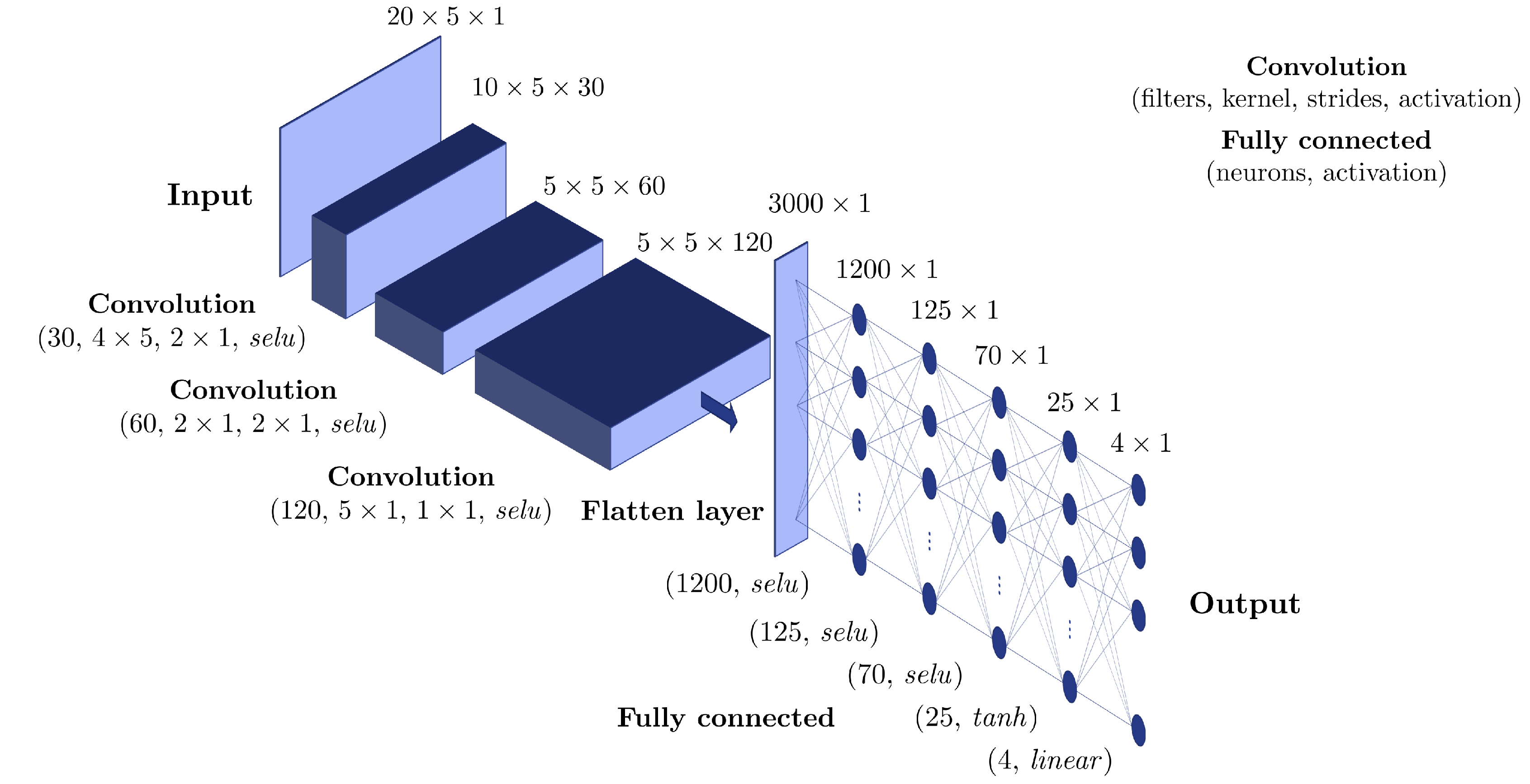
The estimation of h will be done through the use of artificial neural networks. However, since the output consists of $N_t$ evaluations, while the input of $K<N_t$ parameters, a transposed convolution (also known as fractionally-strided convolution) is employed to reach the right dimension at the output layer. As a matter of fact, transposed convolutions increase (up sample) the spatial dimensions of intermediate feature maps, reversing down sample operations obtained by classical convolutions [25].

A second approach consists of considering an incremental modelling framework, in which the model (also known as integrator) computes the next value of the output sequence from a given number of previous inputs and outputs. Such approach has some similarities with the NARXNETs [18]. Denoting with $y_i=y\left(t_i\right)$, for $i=1,\dots ,N_t$, we can write:

$$y_i=h(y_{i-1},y_{i-2},\dots ,y_{i-k},u_i,u_{i-1},\dots ,u_{i-k+1}),$$

(2)

where the parameter $k\ge 0$ is a delay term, known as the process dead time. We can also note $U=y_{past}\cup u$, $y_{past}$ being the known y outputs used to predict future values of y. A neural-network architecture based on a convolution approach can then be defined. Two non-incremental models (for different values of the delay coefficient k) will be compared, in terms of speed and accuracy.

The paper aims to build a data-driven model that is capable of reproducing the data with high fidelity, while possibly performing the integrator task over a large time frame. First of all, the model of the addressed problem and the simulation data structure are described in Section 2. Section 3 presents three different surrogates:

• A non-incremental modelling framework is presented in Section 3.1, which predicts the whole time frame in a single shot
• Two incremental alternatives are presented in Section 3.2. These alternatives used different memory size to predict the future variation in the quantities of interest.
• The incremental surrogate model with large memory is then used as an integrator to predict the variation over a large time series

Finally, Section 4 addresses the conclusion summarizing the results and highlighting the main differences among the learned models.

2. Problem Statement

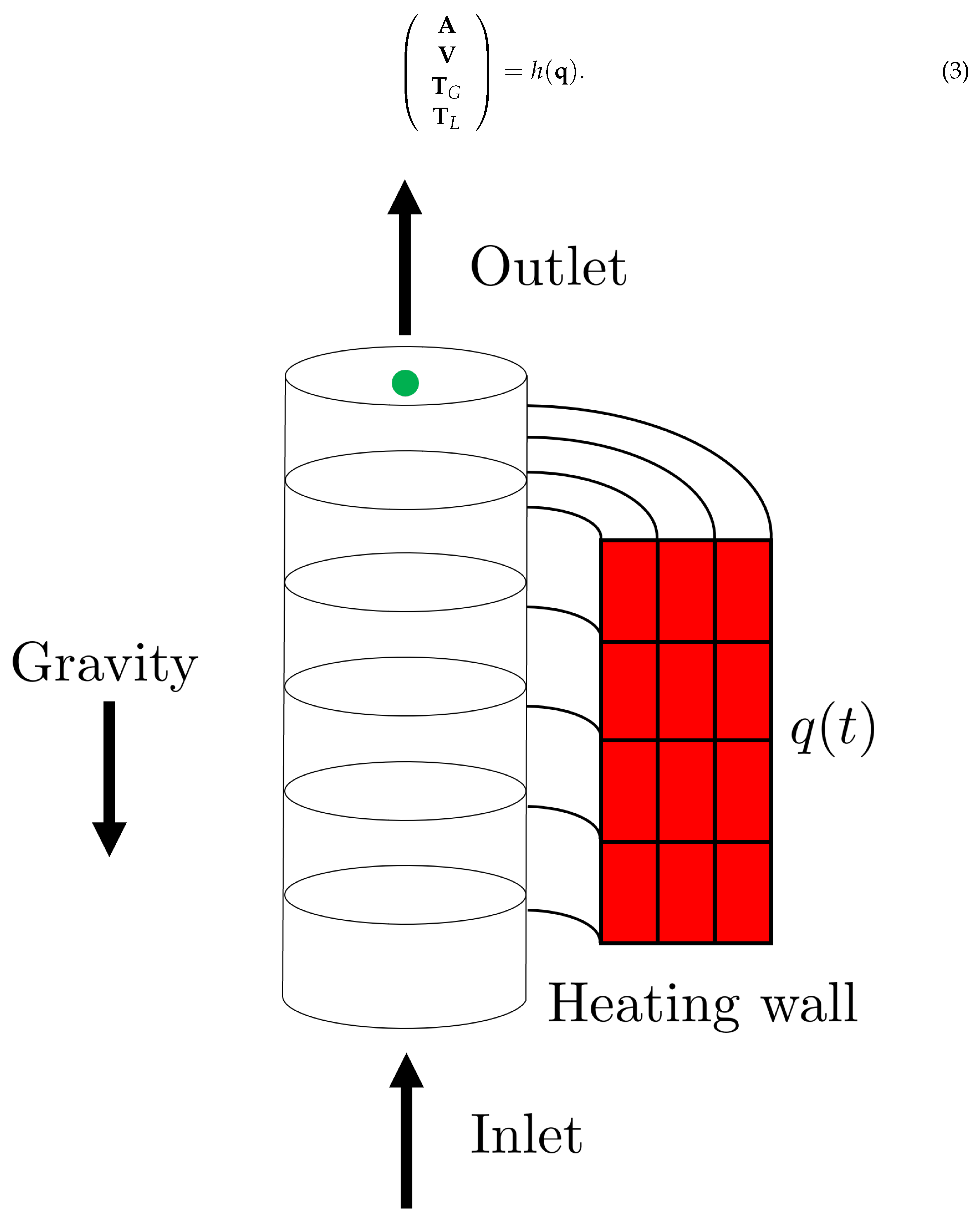
High-fidelity numerical simulations of a thermohydraulic problem are performed using the software CATHARE for nuclear safety analysis [31,32,33]. The simulation consists into a two-phase (steam-water) flow moving upward against gravity into a channel heated by hot walls, as sketched in Figure 1. The model input is the time-varying thermal power $q\left(t\right)$ injected into the fluid through the walls, while the outputs are the time histories of several fluid properties at the channel outlet. The simulation covers the interval $[0,100]$ s, with a time step $\mathrm{\Delta }t=0.1$ s.

Using the bold notation for vectors (sequences of 1000 elements corresponding to the time discretization), the quantities of interest are the steam fraction in the flowing system $\mathbf{A}$, the liquid velocity $\mathbf{V}$, the steam temperature ${\mathbf{T}}_G$ and the liquid temperature ${\mathbf{T}}_L$. This work aims to produce a surrogate model h for inferring the outputs as a function of the input variable $\mathbf{q}$:

$$\left(\begin{array}{c}\mathbf{A}\\ \mathbf{V}\\ {\mathbf{T}}_G\\ {\mathbf{T}}_L\end{array}\right)=h\left(\mathbf{q}\right).$$

(3)

The surrogate model is built in a non-intrusive manner, defining a Design of Experiments–DoE–on the power density and combining the outputs of the corresponding offline simulations.

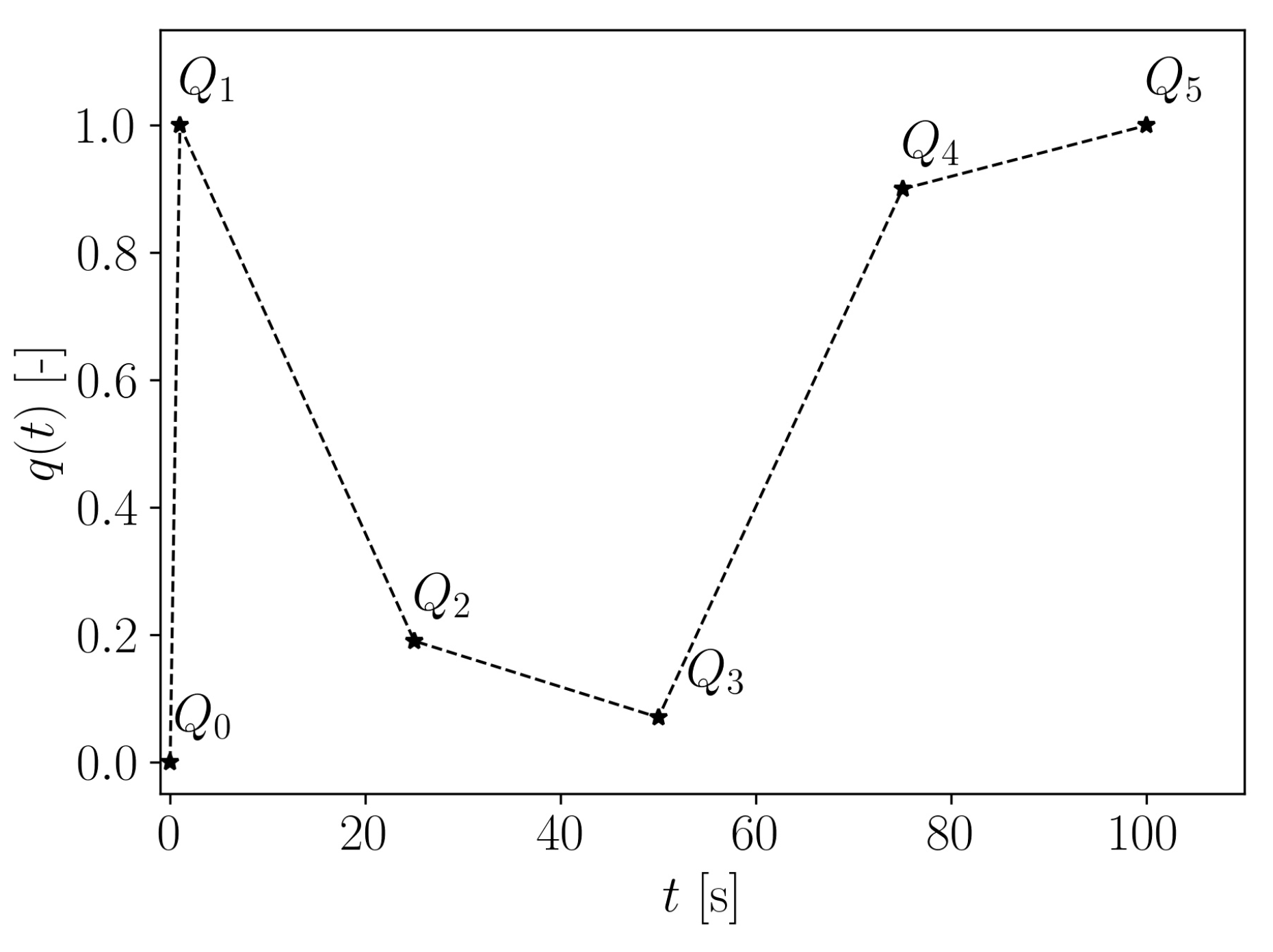
A user-defined power control law allows to assign the value of the provided power density at specific time instants. Therefore, the input function $q\left(t\right)$ is defined through a few values $Q_i=q\left(t_i\right)$, normalized by the maximum power density $Q_{max}=8.4\times {10}^8$ W/m³, and then linearly interpolating in-between. In particular, the time instants (in seconds) $\{0,1,25,50,75,100\}$ are considered for the power changes. The corresponding values $Q_i$, for $i=0,\dots ,5$, define a parametrization of the input function $q\left(t\right)$.

A DoE of 23 data points is established using different combinations of the values $Q_i$, as listed in

Table 1. Available plan of experiment (DoE) and sequences of control points values, as a fraction of $Q_{max}=8.4\times {10}^8$ W/m³.

Sequence Number	${\mathit{Q}}_0$	${\mathit{Q}}_1$	${\mathit{Q}}_2$	${\mathit{Q}}_3$	${\mathit{Q}}_4$	${\mathit{Q}}_5$
1	0	1	0	0	0	1
2	0	1	1	0	0	1
3	0	1	0	1	0	1
4	0	1	0	0	1	1
5	0	1	0	1	1	1
6	0	1	1	0	1	1
7	0	1	1	1	0	1
8	0	1	1	1	1	1
9	0	1	$0.19$	$0.07$	$0.9$	1
10	0	1	$0.06$	$0.8$	$0.28$	1
11	0	1	$0.91$	$0.76$	$0.58$	1
12	0	1	$0.69$	$0.19$	1	1
13	0	1	$0.12$	$0.57$	$0.38$	1
14	0	1	$0.2$	$0.67$	$0.02$	1
15	0	1	$0.99$	$0.92$	$0.47$	1
16	0	1	$0.55$	$0.94$	$0.74$	1
17	0	1	$0.47$	$0.24$	$0.83$	1
18	0	1	$0.76$	$0.36$	$0.18$	1
19	0	1	$0.82$	$0.49$	$0.4$	1
20	0	1	$0.66$	$0.66$	$0.72$	1
21	0	1	$0.31$	$0.43$	$0.6$	1
22	0	1	$0.37$	$0.31$	$0.11$	1
23	0	1	$0.44$	$0.05$	$0.2$	1

. For the rest of this work, the last 4 datasets are considered in the testing set and therefore not fed into the training loop of the built surrogate model. Note that some of the values are fixed ($Q_0=0$, $Q_1=Q_5=1$) thus the model input parameters are only $Q_2,Q_3$ and $Q_4$. Figure 2 shows an example of the heat power density $q\left(t\right)$ defined from values $Q_i$.

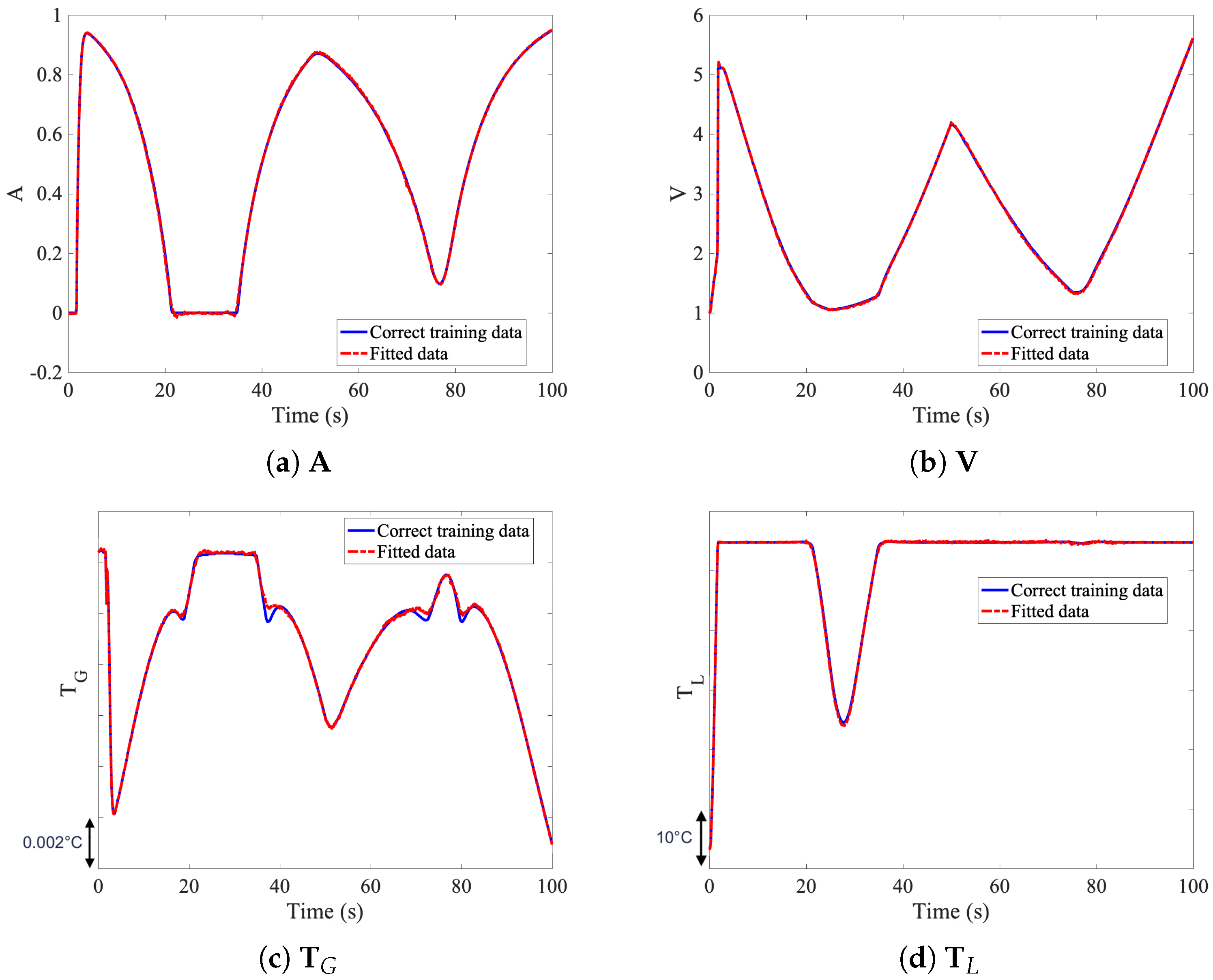
A sample set of results, of the available datasets number 1, 2, 3 and 4 of Table 1, is shown in Figure 3 for illustration purposes.

3. Surrogate Modeling of the Data

Several models are tested and in what follows we explain the results of three of them. Before any training, the variables are normalized by subtracting their corresponding means and dividing by the variation amplitude ${•}_{max}-{•}_{min}$.

3.1. A Non-Incremental Approach

In this section, we present a non-incremental modelling framework, aiming to reproduce all the measured 1000 steps time sequence while considering only the three variables $Q_2$, $Q_3$ and $Q_4$. Therefore, the first model ${\mathcal{H}}_1$ aims to create an output of the form:

$$\left(\begin{array}{c}\widehat{\mathbf{A}}\\ \widehat{\mathbf{V}}\\ \widehat{{\mathbf{T}}_G}\\ \widehat{{\mathbf{T}}_L}\end{array}\right)={\mathcal{H}}_1(Q_2,Q_3,Q_4),$$

(4)

with $\widehat{•}$ being the approximation of the data, output of the surrogate model. In this section, since we are using a non-incremental approach, each dataset is nothing but a single data-point, for which we evaluate a single output. We use a neural network based on a transposed convolution approach [25,26,27]. The network starts with an input of 3 values, for instance (Q₂, Q₃, Q₄), and propagate the variation of the input variables into the required output. The architecture of the used network is illustrated in

Table 2. Structure of the deep convolution transpose neural network used for the fitting of ${\mathcal{H}}_1$. $tanh$ stands for the hyperbolic tangent activation function, $selu$ stands for the scaled exponential linear unit [34], while $linear$ stands for linear activation or no activation function. CT stands for “convolution transpose”.

Layers	Shape	Activation
1	Fully connected dense layer with 7680 neurons	$tanh$
2	Reshape layer into a 3D Tensor of shape $(8\times 4\times 240)$	No activation
3	2D CT, 120 filters, kernel $(5\times 1)$, strides $(5\times 1)$, “same” padding	$selu$
4	2D CT, 60 filters, kernel $(5\times 1)$, strides $(5\times 1)$, “same” padding	$selu$
5	2D CT, 30 filters, kernel $(5\times 1)$, strides $(5\times 1)$, “same” padding	$selu$
6	2D CT, 1 filter, kernel $(1\times 1)$, strides $(1\times 1)$, “same” padding	$linear$

and schematically represented through the diagram in Figure 4. The first layer in the designed neural network transforms the input into a dimension suitable for beginning a convolution transpose. The second layer reshapes the inputs into a simulated 2D picture of dimension 8 × 4, with 240 filters. The subsequent layers reduce the number of filtering while increasing the size of the first dimension of the tensor, through multiplying by 5 on each layer, reaching therefore a dimension of 1000 × 4 on layer 6, the exact dimension of the required 4 variables output.

The neural network is trained over 5000 epochs, with a batch size of 10 datasets, knowing that we have only 19 available datasets. The selected loss function is the mean square error, without regularization, and the optimization algorithm is Adam [35] with an initial learning rate $\alpha ={10}^{-4}$. The results for a selected training dataset are shown in Figure 5, whereas the results for the selected testing datasets are illustrated for datasets 20 and 22 in Figure 6 and Figure 7, respectively.

The relative errors generated by the non-incremental approach are illustrated in

Table 3. Mean relative errors of the trained non-incremental model ${\mathcal{H}}_1$.

Model ${\mathcal{H}}_1$	${\mathcal{E}}_{\mathbf{A}}$	${\mathcal{E}}_{\mathbf{V}}$	${\mathcal{E}}_{{\mathbf{T}}_{\mathit{G}}}$	${\mathcal{E}}_{{\mathbf{T}}_{\mathit{L}}}$
Training sets	0.058%	0.735%	$1.7\times {10}^{-5}$%	0.037%
Testing sets	0.14%	1.61%	$9.0\times {10}^{-5}$%	0.265%

. Since the output $\mathbf{A}$ contains several zero values, the relative error ${\mathcal{E}}_{\mathbf{A}}$ is normalized with respect to the maximum value of $\mathbf{A}$:

$${\mathcal{E}}_{\mathbf{A}}=\frac{\parallel \mathbf{A}-\widehat{\mathbf{A}}{\parallel }_2}{{\parallel \mathbf{A}\parallel }_{\infty }},$$

(5)

with $\mathbf{A}$ being the measured data and $\widehat{\mathbf{A}}$ the surrogate model output. The normalization is standard for any other variable $\mathbf{v}$:

$${\mathcal{E}}_{\mathbf{v}}={∥|\mathbf{v}-\widehat{\mathbf{v}}|\oslash |\mathbf{v}|∥}_2,$$

(6)

where, similarly, $\mathbf{v}$ denotes the measured data, $\widehat{\mathbf{v}}$ the surrogate model output and the symbol ⊘ the Hadamard division operator. The results are excellent in either training or testing sets.

3.2. Incremental Approaches

Using an incremental approach consists in learning the integrator that allows to update the state of the system at each time step. The model is built by first decomposing the datasets into a sequence chain of length $t_s$. Increasing the chain size $t_s$, by considering therefore a higher number of time steps in the variation history, will definitely improve the results, by jeopardizing the computation time required for the prediction of the data point. Two incremental models are tested, the first one considers $t_s=4$, and is an excellent predictor of the next output of the considered sequences but fails as dynamical integrator as will be discussed later, whereas the second model uses $t_s=20$, with a regularization, for improving stability, that performs correctly as integrator.

3.2.1. A Fast Predictor

In this section we explain the possibility of using a fast algorithm based on convolution layers, to predict the next outcome of the sequence at hand. The model will take as an input the variables $(\mathbf{A},\mathbf{V},{\mathbf{T}}_G,{\mathbf{T}}_L)$ at time steps $i-1$, $i-2$, $i-3$ and $i-4$, as well as the input q at time steps i, $i-1$, $i-2$ and $i-3$, to predict the quantities of interest at time step i. For instance, we can write the second trained surrogate model ${\mathcal{H}}_2$ as follows:

$$\left(\begin{array}{c}{\widehat{A}}_i\\ {\widehat{V}}_i\\ {\widehat{T_G}}_i\\ {\widehat{T_L}}_i\end{array}\right)={\mathcal{H}}_2\left(\left(\begin{array}{c}{A}_{i-1}\\ A_{i-2}\\ A_{i-3}\\ A_{i-4}\end{array}\right),\left(\begin{array}{c}{V}_{i-1}\\ V_{i-2}\\ V_{i-3}\\ V_{i-4}\end{array}\right),\left(\begin{array}{c}{T_G}_{i-1}\\ {T_G}_{i-2}\\ {T_G}_{i-3}\\ {T_G}_{i-4}\end{array}\right),\left(\begin{array}{c}{T_L}_{i-1}\\ {T_L}_{i-2}\\ {T_L}_{i-3}\\ {T_L}_{i-4}\end{array}\right),\left(\begin{array}{c}{q}_i\\ q_{i-1}\\ q_{i-2}\\ q_{i-3}\end{array}\right)\right).$$

(7)

The considered network to approximate the surrogate model ${\mathcal{H}}_2$ is summarized in

Table 4. Structure of the deep convolution neural network used for the fitting of ${\mathcal{H}}_2$. $tanh$ stands for the hyperbolic tangent activation function, $selu$ stands for the scaled exponential linear unit [34], while $linear$ stands for linear activation or no activation function.

Layers	Shape	Activation
1	2D convolution, 60 filters, kernel $(2\times 1)$, strides $(2\times 1)$, “same” padding	$selu$
2	2D convolution, 120 filters, kernel $(2\times 1)$, strides $(1\times 1)$, “same” padding	$selu$
3	A flatten layer, reshapes all inputs into a single vector	no activation
4	Fully connected dense layer with 250 neurons	$selu$
5	Fully connected dense layer with 125 neurons	$selu$
6	Fully connected dense layer with 70 neurons	$selu$
7	Fully connected dense layer with 25 neurons	$tanh$
8	Fully connected dense layer with 4 neurons	$linear$

and schematized in Figure 8. The input of the network is a 3D tensor of dimension $(4\times 5\times 1)$, for 4 time steps and 5 variables. The selected optimization algorithm is Adam with the loss function being the mean square errors. The available data after reformulation into a sequence of 4 steps has the size of $19\times 996$ inputs for the training sets and $4\times 996$ for the testing set. A batch size of 996 is selected with 1500 epochs for the training. The initial learning rate was set to $\alpha ={10}^{-4}$.

The results for a selected training dataset are shown in Figure 9, whereas the results for the selected testing datasets are illustrated for datasets 20 and 22 in Figure 10 and Figure 11, respectively. The relative errors are shown in

Table 5. Mean relative errors of the trained incremental model ${\mathcal{H}}_2$ with $t_s=4$. All convolutions employ “same” padding, meaning that the input is half padded and that the filter is applied to all the elements of the input.

Model ${\mathcal{H}}_2$	${\mathcal{E}}_{\mathbf{A}}$	${\mathcal{E}}_{\mathbf{V}}$	${\mathcal{E}}_{{\mathbf{T}}_{\mathit{G}}}$	${\mathcal{E}}_{{\mathbf{T}}_{\mathit{L}}}$
Training sets	0.11%	0.81%	$1.91\times {10}^{-5}$%	0.25%
Testing sets	0.039%	0.898%	$1.94\times {10}^{-5}$%	0.284%

, computed using Equations (5) and (6), as described in Section 3.1.

Model ${\mathcal{H}}_2$ shows an excellent ability to reproduce the datasets when the input is always taken from the physical dataset values and not from the output of the predictor ${\mathcal{H}}_2$ itself. The errors increase dramatically when the input of ${\mathcal{H}}_2$ is taken from its previous output, yielding an impossibility to use it as an integrator of the dynamical system.

On the other hand, the performance of ${\mathcal{H}}_2$ is comparable to the performance of ${\mathcal{H}}_1$, when comparing the relative errors of both models. From a comparison of the resulting graphical illustrations, ${\mathcal{H}}_2$ seems to perform better on the testing sets.

3.2.2. A Larger Sequence Time Integrator

In this section we consider again the rationale followed in Section 3.2.1, with an algorithm based on convolution layers, to predict the next outcome of the sequence at hand. The model will take as an input the variables available at the last 20 time steps. According to the previously introduced notation, $t_s=20$. The built model ${\mathcal{H}}_3$ will predict the quantities of interest at the subsequent time step. For instance, we can write the trained surrogate model ${\mathcal{H}}_3$ as shown below:

$$\left(\begin{array}{c}{\widehat{A}}_i\\ {\widehat{V}}_i\\ {\widehat{T_G}}_i\\ {\widehat{T_L}}_i\end{array}\right)={\mathcal{H}}_3\left(\left(\begin{array}{c}{A}_{i-1}\\ ⋮\\ A_{i-20}\end{array}\right),\left(\begin{array}{c}{V}_{i-1}\\ ⋮\\ V_{i-20}\end{array}\right),\left(\begin{array}{c}{T_G}_{i-1}\\ ⋮\\ {T_G}_{i-20}\end{array}\right),\left(\begin{array}{c}{T_L}_{i-1}\\ ⋮\\ {T_L}_{i-20}\end{array}\right),\left(\begin{array}{c}{q}_i\\ ⋮\\ q_{i-19}\end{array}\right)\right).$$

(8)

The surrogate model ${\mathcal{H}}_3$ is built using the network illustrated in

Table 6. Structure of the deep convolution neural network used for the fitting of ${\mathcal{H}}_3$. $tanh$ stands for the hyperbolic tangent activation function, $selu$ stands for the scaled exponential linear unit [34], while $linear$ stands for linear activation or no activation function.

Layers	Shape	Activation
1	2D convolution, 30 filters, kernel $(4\times 5)$, strides $(2\times 1)$, “same” padding	$selu$
2	2D convolution, 60 filters, kernel $(2\times 1)$, strides $(2\times 1)$, “same” padding	$selu$
3	2D convolution, 120 filters, kernel $(5\times 1)$, strides $(1\times 1)$, “same” padding	$selu$
4	A flatten layer, reshapes all inputs into a single vector	no activation
6	Fully connected dense layer with 125 neurons	$selu$
7	Fully connected dense layer with 70 neurons	$selu$
8	Fully connected dense layer with 25 neurons	$selu$
9	Fully connected dense layer with 4 neurons	$linear$

and represented through the diagram in Figure 12. The input of the network is a 3D tensor of dimension $(20\times 5\times 1)$, for 20 time steps and 5 variables as inputs. The selected optimization algorithm is Adam with the loss function being the mean square errors, modified to add a regularization similar to the DMD regularization [36,37], to perform integration in time without increasing the error significantly. For instance, the loss function $\mathcal{J}$ in this section reads:

$$\begin{array}{c}\mathcal{J}={\displaystyle \sum _{j=1}^{19}}\left(\parallel {\mathbf{A}}_j-\widehat{{\mathbf{A}}_j}\parallel +\parallel {\mathbf{V}}_j-\widehat{{\mathbf{V}}_j}\parallel +\parallel {{\mathbf{T}}_G}_j-{\widehat{{\mathbf{T}}_G}}_j\parallel +\parallel {{\mathbf{T}}_L}_j-{\widehat{{\mathbf{T}}_L}}_j\parallel \right)+\\ +\frac{{\lambda }_w}{2m}{\displaystyle \sum _{j=1}^m}{\theta }_j^2+\frac{{\lambda }_b}{2p}{\displaystyle \sum _{j=1}^p}{\kappa }_j^2\end{array}$$

(9)

where ${\theta }_j$ are all the weights of the last layer of the network described in Table 6 (the linear layer), and ${\kappa }_j$ its biases. ${\lambda }_w$ and ${\lambda }_b$ are regularization parameters. The available data after reformulation into a sequence of 20 steps has the size of $19\times 980$ inputs for the training sets and $4\times 980$ for the testing set. A batch size of 980 is selected with 1500 epochs for the training. The initial learning rate was set to $\alpha ={10}^{-4}$. The input shape has therefore of a size of $20\times 5\times 1$. The results are shown for a ${\lambda }_w={\lambda }_b={10}^{-6}$.

The results using physical inputs for a selected training dataset 10 are shown in Figure 13, whereas the results for the selected testing datasets 20 and 22 in Figure 14 and Figure 15, respectively. The relative errors are shown in

Table 7. Mean relative errors of the trained incremental model ${\mathcal{H}}_3$ with $t_s=20$.

Model ${\mathcal{H}}_3$	${\mathcal{E}}_{\mathbf{A}}$	${\mathcal{E}}_{\mathbf{V}}$	${\mathcal{E}}_{{\mathbf{T}}_{\mathit{G}}}$	${\mathcal{E}}_{{\mathbf{T}}_{\mathit{L}}}$
Training sets	0.058%	1.21%	$9.18\times {10}^{-6}$%	0.039%
Testing sets	0.012%	1.4%	$9.11\times {10}^{-6}$%	0.04%

, computed using Equations (5) and (6), as illustrated in Section 3.1.

3.2.3. Integrator Results

The neural network described in Table 6, complemented with the regularized loss given in Equation (9), can be used to integrate in time the system behavior. For instance, we can write

$$\left(\begin{array}{c}{\widehat{A}}_i\\ {\widehat{V}}_i\\ {\widehat{T_G}}_i\\ {\widehat{T_L}}_i\end{array}\right)={\mathcal{H}}_3\left(\left(\begin{array}{c}{\widehat{A}}_{i-1}\\ ⋮\\ {\widehat{A}}_{i-20}\end{array}\right),\left(\begin{array}{c}{\widehat{V}}_{i-1}\\ ⋮\\ {\widehat{V}}_{i-20}\end{array}\right),\left(\begin{array}{c}{\widehat{T_G}}_{i-1}\\ ⋮\\ {\widehat{T_G}}_{i-20}\end{array}\right),\left(\begin{array}{c}{\widehat{T_L}}_{i-1}\\ ⋮\\ {\widehat{T_L}}_{i-20}\end{array}\right),\left(\begin{array}{c}{q}_i\\ ⋮\\ q_{i-19}\end{array}\right)\right).$$

(10)

The integrator is stable enough to compile all the time steps. Figure 16 shows the integrator results in a training case, whereas Figure 17 and Figure 18 show the integrator results on two testing cases. The integrator errors are given in

Table 8. Mean relative errors of the trained incremental model ${\mathcal{H}}_3$ with $t_s=20$, when performing an integrator operation as per Equation (10).

Model ${\mathcal{H}}_3$	${\mathcal{E}}_{\mathbf{A}}$	${\mathcal{E}}_{\mathbf{V}}$	${\mathcal{E}}_{{\mathbf{T}}_{\mathit{G}}}$	${\mathcal{E}}_{{\mathbf{T}}_{\mathit{L}}}$
Training sets	1.7%	1.54%	$2.07\times {10}^{-5}$%	0.091%
Testing sets	0.44%	1.05%	$2.9\times {10}^{-5}$%	0.045%

.

It can be clearly noticed that the integrator performs extremely well on the selected datasets.

4. Conclusions

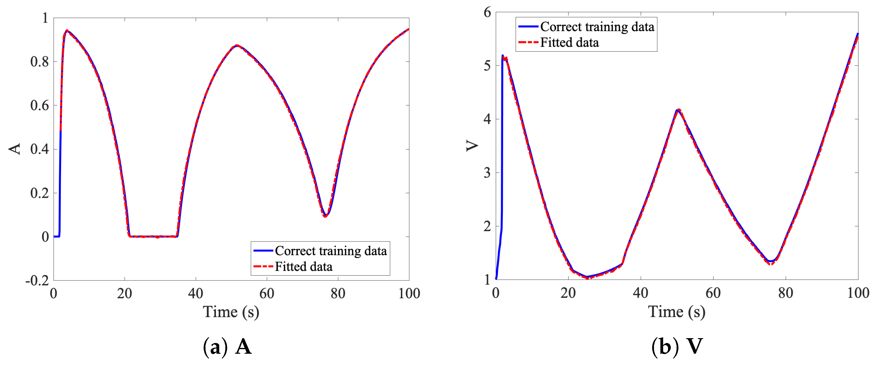
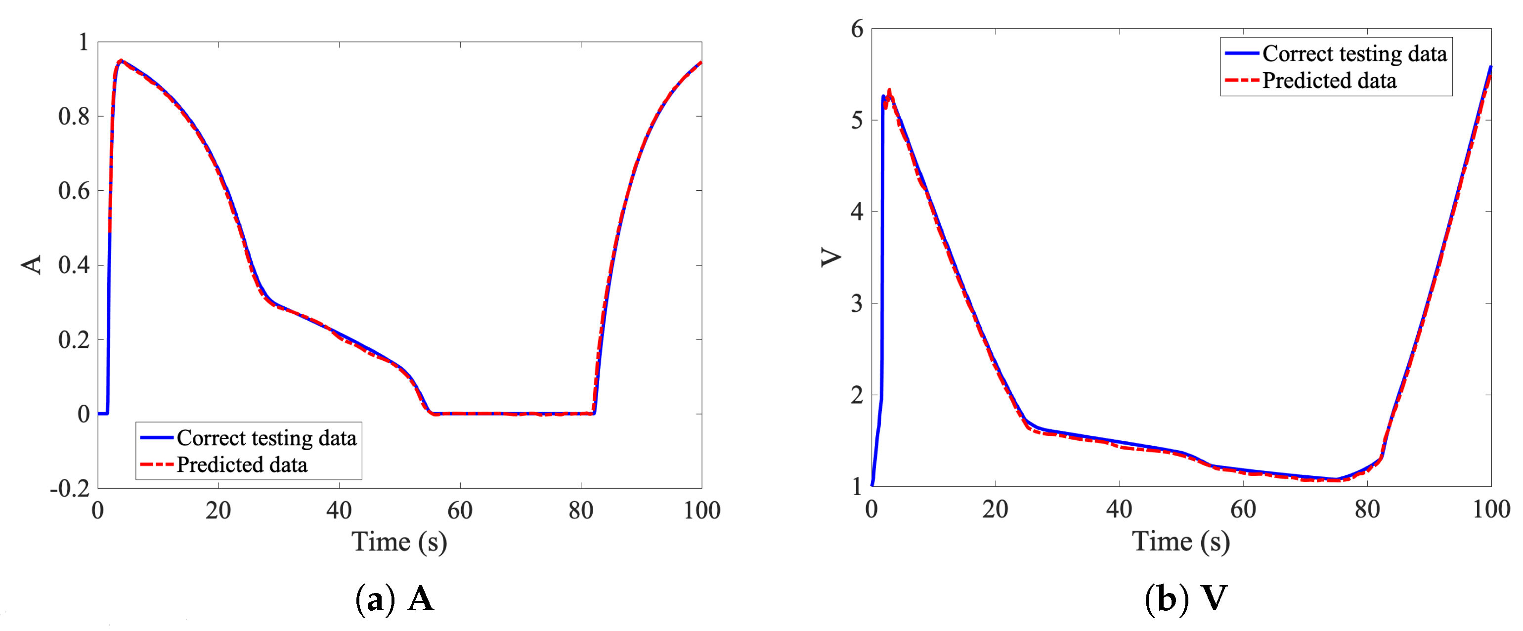
In this work several prediction models for output time series from input time series have been compared. Without loss of generality, a coupled problem in thermohydraulics has been considered, but the procedure generalizes to many other phenomena and fields. Moreover, instead of simulation-based data, experimental data can be used.

The models are based on different deep neural networks architectures. If a parametrization of the input function is available, a non-incremental approach involving transposed convolution neural networks allows the prediction of the whole sequence, as described and discussed in Section 3.1. The non-incremental approach is based on convolution transpose layers, which takes a low amount of data as an input and increase the size of the output to reach a desired dimension. These layers appears as a suitable approach in this situation where only few inputs are required to built the whole sequence of time measurements.

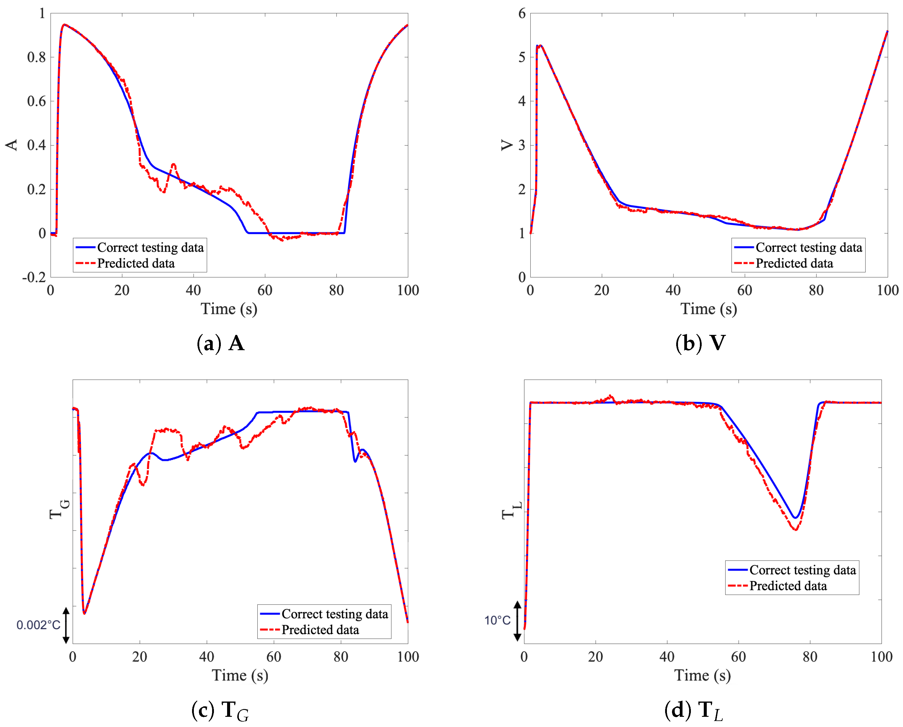
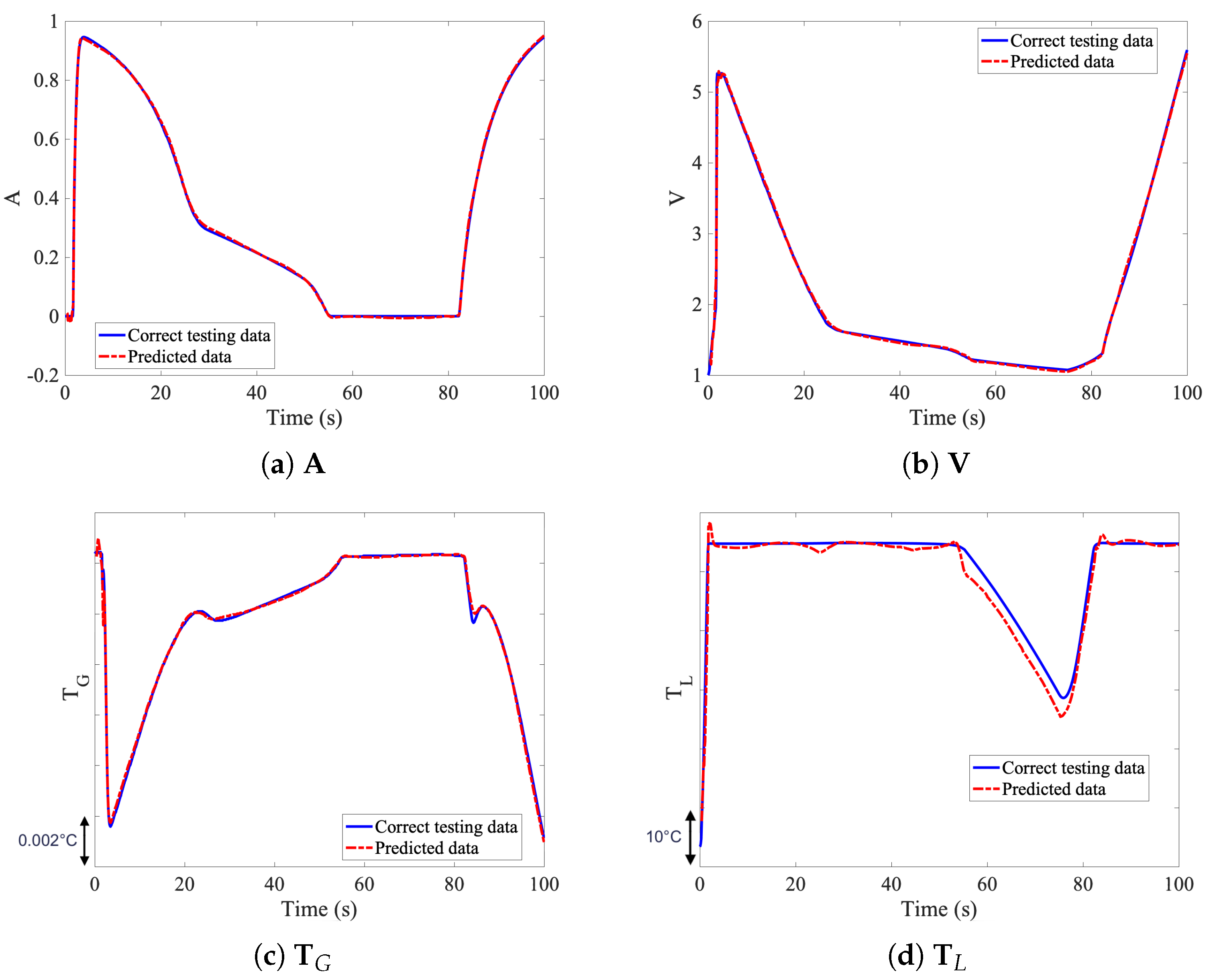
The incremental models (dynamical system integrators) presented in Section 3.2 are based on regressing the variable on its own lagged (i.e., past) values together with the ones of the input, through standard deep convolution neural networks. Therefore, the prediction occurs step-by-step. The difference between the two incremental models stands in the delay (or lag) factor $t_s$. A small value of $t_s$ allows really fast predictions. However, the model can be unstable when its input is taken from the previous model outputs (this occurs, for instance, when $t_s=4$). In such case, the surrogate cannot be used as an integrator of the system. Results are thoroughly improved for $t_s=20$, where also a regularization term was introduced in the loss function. The incremental approach is based on convolution layers. In fact, these layers will take a large input and reduce the input size to extract relevant information. The filters are designed with a large dimension along the time axis, to allow easier extraction of the inputs’ time variation.

The non-incremental approach can be clearly faster to evaluate the output of the solution, however, the integrator clearly outperforms the non-incremental approach. Moreover, the integrator can be used on novel datasets, and potentially outside of the simulated time frame. The initialization requires only $t_s$ time-steps to be simulated, and the remaining dynamics is predicted in real time, allowing huge computational gains. However, the non-incremental approach can’t be used on a different time frame, out of the simulated region, as the output is hardly coded to predict only $N_t=1000$ time steps.