Imprecise Bayesian Networks as Causal Models

Abstract

This article considers the extent to which Bayesian networks with imprecise probabilities, which are used in statistics and computer science for predictive purposes, can be used to represent causal structure. It is argued that the adequacy conditions for causal representation in the precise context—the Causal Markov Condition and Minimality—do not readily translate into the imprecise context. Crucial to this argument is the fact that the independence relation between random variables can be understood in several different ways when the joint probability distribution over those variables is imprecise, none of which provides a compelling basis for the causal interpretation of imprecise Bayes nets. I conclude that there are serious limits to the use of imprecise Bayesian networks to represent causal structure.

1. Introduction

Probabilistic models in many scientific contexts are often characterized by ambiguity. Consider the following real-world example, due to [1]. Geologists in the Ticino canton in southern Switzerland want to know how likely it is that a debris flow in a given region will be of low, medium, or high severity, given certain information about the geomorphology of a region. A debris flow is a geological incident that is similar to a mudslide. A low-severity flow is one in which the thickness of the debris displaced is less than 10 $\mathrm{cm}$, a medium-severity flow is one in which the thickness of the debris displaced is between 10 $\mathrm{cm}$ and 50 $\mathrm{cm}$, and a high-severity flow is one in which the thickness of the debris displaced is greater than 50 $\mathrm{cm}$. A statistical model representing the relationship between the geomorphology of a region and the severity of a debris flow contains several input variables, such as land use and antecedent soil moisture. Scientists are uncertain as to the values of these variables, and they are also uncertain about the extent to which these values influence the probability distribution over the severity of a debris flow. The model reflects this uncertainty by assigning probability intervals, rather than precise probabilities, to each of the possible debris flow outcomes. To illustrate, for one set of inputs, Antonucci et al.’s model determines that the probability of a low-severity flow is in the interval $[0.08,0.30]$, that the probability of a medium-severity flow is in the interval $[0.23,0.32]$, and that the probability of a high severity flow is in the interval $[0.46,0.69]$ ([1], p. 7). (In the example cited, these probability intervals are calculated using the imprecise Bayes nets techniques discussed in this paper.)

It is plausible that the inherent ambiguity of these probabilistic outputs is a feature, not a bug, of the model that generates them. As Joyce [2] argues, there are cases in which agents ought to have imprecise degrees of belief with respect to future outcomes, since their total evidence does not warrant the assignment of a precise probability to any particular outcome (See [3] for a full accounting of the various reasons discussed in the literature for adopting epistemic attitudes best represented by imprecise probabilities). I take it that the geological case described above falls into this category. Indeed, Antonucci et al. claim that the use of probability intervals, as opposed to precise probabilities, allows them to “quantify uncertainty on the basis of historical data, expert knowledge, and physical theories” ([1], p. 1). Further, the uncertainty regarding the relationships between various inputs and the severity of a debris flow is such that one cannot define a second-order probability distribution over the interval range. Thus, it does not make sense to take an average over the interval and arrive at a single, precise probability. Rather, the imprecise judgments produced by the model may well represent the epistemic attitude that is most warranted by the available evidence.

Bayesian network models, such as those developed by Pearl [4] and Spirtes et al. [5], provide powerful tools for representing the causal structure of the world. Traditionally, these models exclusively use precise probabilities. Thus, it is an important question whether extensions of these models that allow for imprecise probabilities will yield similar fruit. Most work on imprecise Bayesian networks (IBNs) has occurred in the statistics and computer science literature (see [6] for a comprehensive overview) (In the computer science and statistical literature, IBNs are sometimes called credal networks). I avoid this term here because of the different usage of the term “credence” in formal epistemology. Unsurprisingly, this literature has focused largely on the use of IBNs to make predictions about future events. By contrast, there has been little attention focused on the philosophical issue of whether and to what extent IBNs can be used to represent the causal structure of actual systems; that is, whether the edges in an IBN can be interpreted as type-level causal relations between variables.(The meaning of “edge” and “variable” in this context will be made precise in the next section). Addressing this issue is my focus in this paper.

My central task is to determine whether and how the Causal Markov Condition (CMC) and the Minimality condition—which are individually necessary and jointly sufficient conditions for the causal interpretation of a Bayesian network—can be extended into the imprecise context. In general, determining whether a Bayes net satisfies CMC and Minimality requires an understanding of what it means for two random variables to be independent of one another. In the precise context, such independence has only one mathematical definition, but in an imprecise context, multiple independence concepts abound (see [7,8]). Most saliently, imprecise probability distributions over different variables may satisfy so-called strong independence, or the weaker notion of epistemic independence. In what follows, I argue that neither strong nor epistemic independence can be neatly “plugged in” to CMC and Minimality to yield a compelling set of adequacy conditions for the causal interpretation of IBNs without troubling implications. These implications can be avoided by positing further restrictions on the probabilistic features of IBNs, but such restrictions demonstrate the extent to which many otherwise innocuous imprecise probabilistic models cannot be interpreted causally. Thus, I conclude that introducing imprecision into probabilistic graphical models can limit their ability to represent causal structure.

My plan for this paper is as follows. In Section 2, I present the basic formalism for precise Bayesian network models, show how CMC and Minimality license a causal interpretation of those models, and describe the central role that probabilistic independence plays in defining these conditions. In Section 3, I present the basic formalism for IBNs. In Section 4, I illustrate the distinction between strong and epistemic independence between random variables in an imprecise probabilistic context. In Section 5, I argue that neither strong nor epistemic independence can be used to adapt CMC and Minimality into an imprecise context. In Section 6, I consider and respond to some salient objections to my argument. In Section 7, I offer concluding remarks.

2. Precise Bayes Nets as Causal Models

A Bayes net is triple $\mathcal{G}=\langle \mathcal{V},\mathcal{E},P\rangle$. $\mathcal{V}$ is set of random variables whose values denote different possible states of the system being represented. $\mathcal{E}$ is an acyclic set of ordered pairs of the variables in $\mathcal{V}$. These ordered pairs, called “edges”, are usually represented visually as arrows pointing from one variable to another. If a graph contains an edge $V_1\to V_2$, then $V_1$ is a parent of $V_2$, and $V_2$ is a child of $V_1$. A chain of parent–child relationships is called a directed path. If there is a directed path from a variable $V_3$ to a variable $V_4$, then $V_4$ is a descendant of $V_3$ and $V_3$ is an ancestor of $V_4$. Together, these sets of variables and edges comprise the graph $\langle \mathcal{V},\mathcal{E}\rangle$, which represents the causal structure of a given system. A joint probability distribution P is defined over the variables of the graph. This joint distribution can be used to derive the conditional probability that each variable in the graph takes some value, given some setting of values for any combination of variables in the graph, as well as marginal probability distributions over all of the variables in the graph. Extreme probabilities can be used to give a deterministic representation of a causal system. At this point, we assume that all probability distributions in the Bayes net are precise, meaning that they assign a single numerical value to each event in the measure space of the variables that they are defined over.

We want to be able to interpret a Bayes net causally. A causal interpretation is one that takes the parent–child relationship to represent a direct causal relevance relation between two variables, with each parent variable directly causing its children. Following Ref. [9], I will not attempt to give a reductive account of direct causation, but will instead show that certain probabilistic constraints on a Bayes net ensure that the parent–child relationship satisfies intuitive constraints on any notion of direct causation (Elsewhere, Woodward [10] gives an account of direct causation in terms of interventions. This account is also non-reductive, in that interventions on variables are themselves defined using the concept of direct causation). The core tenet of the causal modelling literature is that, to represent causal relationships, a Bayes net must satisfy the Causal Markov Condition, which is defined as follows.

Causal Markov Condition (CMC): For any variable X in $\mathcal{G}$, the value of X is independent of its non-descendants, conditional on its parents.

At first glance, the connection between CMC and the causal interpretation of a Bayes net is opaque. However, this connection can be rendered more obvious by considering two crucial consequences of CMC, namely the way in which parents screen off their children from other variables, and the way in which correlations between variables that are not causally related can be accounted for by considering the common parents of those variables.

Let us begin with screening off. According to this condition, any representation of direct causation should entail that, once we have full information about all the causes of an event, no additional information about the causes of those causes should change the probability that we assign to an event. More formally, let us define the screening off condition as follows.

Screening Off: For any variable X in $\mathcal{G}$, if ${\mathcal{PA}}_X$ is the set containing all the parents of X and W is a parent of some variable in ${\mathcal{PA}}_X$, then X and W are independent, conditional on ${\mathcal{PA}}_X$.

To illustrate, consider the simple causal graph in Figure 1, in which each variable takes the value 1 or 0 depending on whether the indicated factor is absent or present in a given person. Screening Off says that, once we know the value of the variable Smoking, the probability that the person has lung cancer is independent of the value of Stress. Thus, the parent–child relationship plays the screening-off role that we require of any notion of direct causation.

The second important corollary of CMC is closely related to Reichenbach’s [11] “common cause” condition. This condition states that any correlation between two variables can be explained by showing a chain of direct causal relations from one variable to another, or by tracing the causal history of both variables back to a common ancestor. This can be stated in graph-theoretic terms as follows.

Common Cause: For any disjoint sets of variables $\mathcal{X}$ and $\mathcal{Y}$ in $\mathcal{G}$, if $\mathcal{X}$ and $\mathcal{Y}$ are not unconditionally independent, then there exists a pair of variables $X\in \mathcal{X}$ and $Y\in \mathcal{Y}$ such that either one variable is a descendant of the other, or X and Y have at least one shared ancestor $A_{X,Y}$ such that X and Y are independent conditional on $A_{X,Y}$.

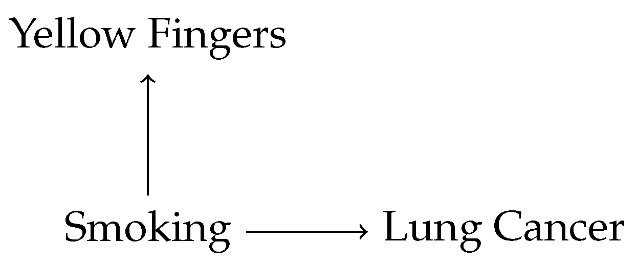
To illustrate, consider the graph in Figure 2. Again, all variables are binary and denote the presence or absence of yellow teeth, smoking, or lung cancer. Suppose that there is an observed correlation between Yellow Fingers and Lung Cancer; unconditionally, the two variables are not independent. If, as is likely the case, there is no direct causal link in either direction between Yellow Fingers and Lung Cancer, Common Cause tells us that the two variables must share a common ancestor, viz. Smoking, on which they are conditionally independent.

Screening Off and Common Cause exhaust the logical content of CMC. That is, the following proposition is true (see Appendix A for proof):

Proposition 1.

A graph $\mathcal{G}$ satisfies CMC if and only if it satisfies Screening Off and Common Cause.

The connection between these three conditions is well-established, such that the truth of this proposition is not a novel result. The content of the result can largely be found in [12], and in similar results by [13,14]. However, this unambiguous connection between CMC and two intuitive necessary conditions for interpreting the parent–child relationship as one of direct causation is rarely stated in these concrete terms.

CMC alone is not sufficient for the causal interpretation of a Bayes net. To see why, consider a simple Bayes net of the form $X\to Y\to Z$. If we suppose that the variables X, Y, and Z are all independent of one another, then this Bayes net trivially satisfies CMC; if all three variables are independent of each other, then they are each by implication independent of their non-descendants, conditional on their parents. However, since the three variables are independent, they cannot be causally related to each other in the manner suggested by the ordering of edges in this graph. Thus, a further condition is required to ensure the sufficiency of a Bayes net for causal interpretation. The weakest such condition proposed in the literature is the Minimality condition [5], which can be stated as follows.

Minimality: For any graph $\mathcal{G}$, there is a subgraph ${\mathcal{G}}^{*}$ that differs from $\mathcal{G}$ solely with respect to a single edge that is included in $\mathcal{G}$ but absent from ${\mathcal{G}}^{*}$. A graph $\mathcal{G}$ satisfies Minimality if and only if no such subgraph ${\mathcal{G}}^{*}$ satisfies the Causal Markov Condition.

A Bayes net that satisfies Minimality contains no extraneous edges. That is, there are no arrows between any two variables such that those two variables are independent conditional on their parents. Thus, if the variables X, Y, and Z are all independent of one another, then the graph $X\to Y\to Z$ does not satisfy Minimality. This is because any of the arrows in the graph can be removed without creating a sub-graph that violates CMC. If we hold that Screening Off and Common Cause are the only two conditions that we require a primitive notion of direct causation to satisfy, then CMC and Minimality are individually necessary and jointly sufficient conditions for the causal interpretation of Bayes net, since they ensure that all parent–child relationships in the graph play one of the two roles that we want any representation of a direct causal relationship to play (Many readers will be familiar with the Faithfulness condition for Bayes nets, which is strictly stronger than Minimality. I choose Minimality over Faithfulness as an adequacy condition for the causal interpretation of Bayes nets, since there is a case to be made that Bayes nets that satisfy Minimality but not Faithfulness are accurate representations of some causal systems. For a perspicuous comparison of the two conditions, see [15]).

Thus, if a Bayes net satisfies CMC and Minimality, we can interpret its arrows causally. Note, however, that the fact that satisfying CMC and Minimality licenses a causal interpretation of a Bayes net does not entail that any Bayes net that satisfies these conditions provides a correct representation of a particular system. To see this, suppose that the variables X, Y, and Z are all correlated with one another. The graphs $X\to Y\to Z$ $X\leftarrow Y\leftarrow Z$, and $X\leftarrow Y\to Z$, among others, will all satisfy CMC and Minimality. To determine which graph is correct, we will need to perform experiments; for example, if we exogenously fix the value of the variable X and this changes the probability distribution over Z, then $X\to Y\to Z$ is the correct graph of the three listed above. While the discovery of the correct causal graph using interventions is an important part of the literature on causal Bayes nets, I bracket this discussion for the remainder of this paper. What is important for my purposes is that, because they satisfy CMC and Minimality, all three of these graphs can be interpreted as hypotheses about the causal structure of the world.

However, Bayes nets methods can yield some unambiguous conclusions regarding the causal structure of target systems. Let $(X,Y)$ be a pair of adjacent variables in a Bayes net $\mathcal{G}$ if and only if $\mathcal{G}$ contains an edge $X\to Y$ or an edge $Y\to X$. [12] prove that if two Bayes nets share the same variable set $\mathcal{V}$ and the same joint probability distribution P, then they share the same pairs of adjacent variables. Thus, for any given precise probability distribution P and variable set $\mathcal{V}$, all Bayes nets that are consistent with P will agree with respect to which variables are directly causally related and which variables are not. The ambiguity as to the correct Bayes net, given the joint probability distribution over $\mathcal{V}$, is solely a matter of the direction of the direct causal relationship between two variables; there is no ambiguity as to whether such a relationship exists. To put this another way, if it were to turn out to be the case that no direct causal connection in fact exists between two variables related by a direct edge in a Bayes net, it would have to be the case that either of two conditions obtains: (1) there is a failure of causal sufficiency, i.e., there are latent variables that have not been included in the Bayes net (A precise definition of causal sufficiency is as follows. For any variable X that is not in $\mathcal{V}$, the joint probability assigned to all variables in $\mathcal{V}$ is the same for all values of X ([5], p. 475)); or (2) the probability distribution over the existing variables is inaccurate. Similarly, if there is a direct causal connection between two variables that are not related by a directed edge, then there is a either a failure of causal sufficiency or the joint probability distribution over the graph is inaccurate. This important feature of Bayes nets turns out not to hold in the imprecise context, and this contrast between precise and imprecise Bayes nets will be important to my subsequent analysis.

This analysis helps itself to the existence of a model-independent fact of the matter as to whether there is a causal relationship between two variables. Though the nature of such model-independent causal relationships is a topic well beyond the scope of this paper, for the sake of argument, I adopt a mechanistic understanding of such relationships; one variable directly causes another if there is a direct mechanistic connection between changes in the value of one variable and changes in the value of the other. Following Ref. [16], I understand mechanisms as “entities and activities organized such that they are productive of regular changes from start or set-up to finish or termination conditions” ([16], p. 3). As such, a mechanistic connection between two variables means that, in the actual world, there are entities and activities organized such that changing the value of one variable leads to regular changes in the probability distribution over another variable. A direct mechanistic connection is one that holds independently of the values taken by the other variables in the graph. This is a decidedly counterfactual or interventionist understanding of the meaning of “productive”, in keeping with the understanding of mechanisms advanced by Woodward [17]. This stands in contrast to a more ontic notion of productivity advocated by Glennan [18], according to which productivity in mechanisms requires a physical process connecting the components of a mechanism.

Before moving to discuss Bayes nets with imprecise probabilities, I must first address the concept of probabilistic independence between random variables. Obviously, probabilistic independence plays a crucial role in our understanding of CMC and Minimality, since independence is part of the very definition of CMC. Therefore, one must understand the relation of independence between random variables in order to understand the causal interpretation of a Bayes net. Where all probabilities are assumed to be precise, independence has a straightforward mathematical meaning, which can be stated as follows.

Precise Unconditional Independence:X and Y are independent if and only if, for all values x and y, $P(X=x,Y=y)=P(X=x)·P(Y=y)$.

Similarly, conditional independence in the precise probabilistic context can be defined as follows.

Precise Conditional Independence:X and Y are independent conditional on Z if and only if, for all values x, y and z, $P(X=x,Y=y|Z=z)=P(X=x|Z=z)·P(Y=y|Z=z)$.

Different modellers may hold that different statistical hurdles have to be cleared to license the conclusion that there is dependence or independence between two variables. For example, different modellers may hold that data must support the existence of a dependence relation between two variables at a certain level of statistical significance. Nevertheless, where precise probabilities are used, the mathematical definitions of independence and conditional independence are just those given above.

3. Imprecise Bayes Nets: The Basics

Following Ref. [6], I define an imprecise Bayes net as a triple $\mathcal{I}=\langle \mathcal{V},\mathcal{E},\mathcal{K}\rangle$. As in a precise Bayes net, $\mathcal{V}$ is a set of variables and $\mathcal{E}$ is a acyclic set of directed edges. However, whereas a precise Bayes net contains a joint probability distribution P, an imprecise Bayes net contains a set of joint probability distributions $\mathcal{K}$. That is, $\mathcal{K}$ maps every possible combination of values for all of the variables in the graph to a set of possible probabilities for that combination of values. As in the precise context, we can use $\mathcal{K}$ to derive sets of conditional and marginal probabilities over the variables in the graph. Following Ref. [19,20], I call these sets of probability distributions over variables “credal sets”. For example, if X is a variable in an IBN, then the set of marginal probability distributions over X that is implied by the joint distribution $\mathcal{K}$ is the credal set for X. If Y is another variable in the graph, then the set of conditional probability distributions over X, given that $Y=y$, is the conditional credal set over X, given that $Y=y$.

To illustrate via a toy example, suppose that an IBN contains a binary variable S denoting whether a person smokes, and another binary variable $LC$ denoting whether they develop lung cancer. If the probability that someone develops lung cancer, given that they smoke, is best represented by the interval $[0.05,0.2]$, then we can define the the following conditional credal set over $LC$, given $S=1$ (i.e., given that the person smokes):

$${\mathcal{K}}_{S=1}=\{P:P(LC=1|S=1)\in [0.05,0.2],P(LC=0|S=1)\in [0.8,0.95]\}$$

(1)

This is the set of all precise probability distributions over $LC$, given $S=1$, such that any probability $P(LC=1|S=1)$ that is consistent with ${\mathcal{K}}_{S=1}$ takes a precise value within the interval $[0.05,0.2]$, and such that any probability $P(LC=0|S=1)$ that is consistent with ${\mathcal{K}}_{S=1}$ takes a precise value within the interval $[0.8,0.95]$. From this element-by-element, or pointwise, analysis of the credal set, we can infer the interval-valued claim that the probability of lung cancer, given smoking, is in the interval $[0.05,0.2]$.

This method of representing imprecise probabilities as sets of probability distributions has its roots in foundational works by Levi [19,20] and Walley [21]. However, unlike these authors, I do not assume that all credal sets are convex. That is, I drop the assumption that for any two probabilities in the credal set, the linear average of these two probabilities is also in the credal set. While perhaps non-standard, the decision to eschew the convexity requirement for credal sets has some precedent in the recent literature; see for instance [22,23].

To interpret an IBN causally, we will need to extend the notions of unconditional and conditional independence between variables to apply to cases where there is not a precise joint probability distribution over all pairs of variables in a graph, but where there is a specified family of joint probability distributions over the variables in a graph. This would allow us to define imprecise extensions of the CMC and Minimality conditions. However, as described in Section 1, there is no single notion of what it means for two variables to be independent when independence is defined in terms of imprecise probabilities. In the next section, I outline the two leading ways of cashing out independence in an imprecise context: strong independence and epistemic independence. I show that there are substantive differences between the two notions of independence, with important consequences for the causal interpretation of IBNs.

4. Two Concepts of Independence

4.1. Strong Independence

The most natural extension of the concept of probabilistic independence into the imprecise context is via the notion of strong independence, which “has been adopted by most of the authors who have modeled independence using imprecise probabilities” ([7], p. 7). A simple statement of strong independence is as follows. First, for two variables X and Y, we define a set of probability distributions $\mathcal{SI}$:

$$\mathcal{SI}=\{P:P(X=x,Y=y)=P(X=x)·P(Y=y\left)\right\}$$

(2)

This is the set of all joint probability distributions such that the fact that $X=x$ is independent of the fact that $Y=y$. It is worth noting here that most discussions of independence in the imprecise context would define $\mathcal{SI}$ as the convex hull of the set $\{P:P(X=x,Y=y)=P(X=x)·P(Y=y\left)\right\}$, i.e., the smallest convex set containing the set $\{P:P(X=x,Y=y)=P(X=x)·P(Y=y\left)\right\}$. This move has its roots in [20], and is required in order to maintain the convexity of credal sets, as the set $\{P:P(X=x,Y=y)=P(X=x)·P(Y=y\left)\right\}$ is not generally convex. However, since I do not require that credal sets be convex, this further stipulation is unnecessary here. Having defined this set, we can define strong independence as follows.

Strong Independence:X and Y are strongly independent if and only if, for all values x and y, $\mathcal{K}(X=x,Y=y)\subseteq \mathcal{SI}$.

To illustrate, consider the graph in Figure 3, on which the z-axis values represent the joint probability $P(X=x,Y=y)$ and the x and y axis values represent the marginal probabilities $P(X=x)$ and $P(Y=y)$, respectively. The surface shown in the graph is the set of joint probabilities such that $P(X=x,Y=y)=P(X=x)·P(Y=y)$. If the set of joint probabilities $\mathcal{K}(X=x,Y=y)$ is a subset of this set for all values x and y, then X and Y are strongly independent.

These definitions can be straightforwardly augmented to provide definitions of conditional independence. First, we define a set of joint conditional probabilities $\mathcal{CSI}$:

$$\mathcal{CSI}=\{P:P(X=x,Y=y|Z=z)=P(X=x|Z=z)·P(Y=y|Z=z)\}$$

(3)

This allows us to define conditional strong independence as follows.

Conditional Strong Independence:X and Y are strongly independent conditional on Z if and only if, for all values x, y, and z, $\mathcal{K}(X=x,Y=y|Z=z)\subseteq \mathcal{CSI}$.

It should be clear from the previous section that this notion of conditional strong independence will be crucial for understanding how the CMC and Minimality conditions can be extended into the imprecise context, if strong independence is taken to be the operative independence concept for a causal interpretation of an imprecise Bayes net.

Strong independence can also be understood as a pointwise notion of independence. Recall that the joint credal set over X and Y is a set of precise joint probability distributions. Strong independence requires that every element (or “point”) in this set satisfy the precise version of independence or conditional independence. As I demonstrate shortly, this same pointwise analysis is not applicable to all notions of independence in the imprecise context.

4.2. Epistemic Independence

A rival notion of independence between two random variables in the imprecise context is the notion of epistemic independence; according to Walley [21], this is the correct way of understanding independence between variables in an imprecise context. To define epistemic independence, we begin by letting $\mathcal{K}(X=x)$ be a set of marginal probabilities assigned to $X=x$, and letting $\mathcal{K}(Y=y)$ be a set of marginal probabilities assigned to $Y=y$. Next, we define a set of probabilities $\mathcal{EI}$:

$$\mathcal{EI}=\{P:P(X=x|Y=y)\in \mathcal{K}(X=x),P(Y=y|X=x)\in \mathcal{K}(Y=y\left)\right\}$$

(4)

$\mathcal{EI}$ contains the set of all conditional probability distributions such that conditionalizing on the fact that $Y=y$ does not move the probability that $X=x$ outside of its marginal range, and such that conditionalizing on the fact that $X=x$ does not move the probability that $Y=y$ outside of its marginal range. In other words, epistemic independence holds that the value of Y is epistemically irrelevant to the agent’s credal set over X, and that the value of X is epistemically irrelevant to the agent’s credal set over Y. Having defined $\mathcal{EI}$, we can define epistemic independence as follows.

Epistemic Independence:X and Y are epistemically independent if and only if, for all values x and y, $\mathcal{K}(X=x|Y=y)\subseteq \mathcal{EI}$ and $\mathcal{K}(Y=y|X=x)\subseteq \mathcal{EI}$.

These definitions can be straightforwardly adapted to the conditional context. First, we define the set of conditional probabilities $\mathcal{CEI}$:

$$\mathcal{CEI}=\{P:P(X=x|Y=y,Z=z)\in \mathcal{K}(X=x),P(Y=y|X=x,Z=z)\in \mathcal{K}(Y=y\left)\right\}$$

(5)

This leads directly to the following definition of conditional epistemic independence:

Conditional Epistemic Independence:X and Y are epistemically independent conditional on Z if and only if, for all values x, y, and z, $\mathcal{K}(X=x|Y=y,Z=z)\subseteq \mathcal{CEI}$ and $\mathcal{K}(Y=y|X=x,Z=z)\subseteq \mathcal{CEI}$.

These definitions lay the groundwork for a possible causal interpretation of IBNs in which epistemic independence is the operative independence concept.

Determining whether a given joint probability distribution is within the set of joint distributions that satisfy epistemic independence is computationally difficult, requiring multi-linear programming techniques (see [24]). Further, unlike strong independence, epistemic independence does not impose a particular independence condition on every element of the joint credal set. That is, it is not a pointwise notion of independence. Rather, it is a setwise notion of independence, requiring only that the whole joint credal set $\mathcal{K}$ is such that all of the conditional probability distributions over each variable that are consistent with $\mathcal{K}$ are within all of the marginal probability distributions over each variable that are consistent with $\mathcal{K}$.

4.3. Distinguishing the Two Independence Concepts

Strong independence is a strictly stronger condition on the probabilistic relationship between two variables than epistemic independence (see [7] for a demonstration of this point). This means that strong independence implies epistemic independence, but not vice versa. However, more interesting distinctions between the two concepts can also be drawn. Namely, satisfying strong independence seems to require the lack of a mechanistic connection relation between the values of two variables. By contrast, satisfying epistemic independence requires a purely informational or evidential independence between the two variables. That is, if two variables are epistemically independent, then learning the value of either variable should not change the behavior of an agent, where that behavior depends on the value of the other variable (e.g., deciding how much to gamble on the value of either variable). To illustrate this distinction, consider the following toy case, which is adapted from [7] (Note that [7] is concerned with notions of independence in the imprecise context but not with imprecise Bayes nets):

Urn Example: There are three urns, A, B, and C, each of which contain 100 balls. The balls in each urn are either red or white. Urn A contains 50 red balls, 20 white balls, and 30 balls that are either red or white. Urns B and C each contain 30 red balls, 30 white balls, and 40 that are either red or white. We begin by drawing a ball from Urn A. If the ball drawn from Urn A is red, then we draw a second ball from Urn B. If the ball drawn from Urn A is white, then we draw a second ball from Urn C. Once it is decided which urn to draw from, each ball in that urn is equally likely to be drawn. Let F be a variable whose values denote the color of the first ball drawn, and let S be a variable whose values denote the color of the second ball drawn. Let u be the number of red balls in Urn B, and let v be the number of red balls in Urn C.

The following proposition is true:

Proposition 2.

The variables F and S in Urn Example are strongly independent if and only if $u=v$.

This result fits with the idea that if an agent’s imprecise joint credal set over two variables satisfies strong independence, then that agent ought to believe in the absence of a mechanistic connection between the phenomena represented by the two variables. In this case, if an agent’s imprecise joint credal set over F and S satisfies strong independence, then that agent also ought to believe that $u=v$.

By contrast, we can give cases in which F and S are epistemically independent, but $u\ne v$. To illustrate, let us begin by defining marginal credal sets over F and S. Given that there are between 50 and 80 red balls in Urn A, and between 30 and 70 red balls in Urns B and C, these credal sets should be defined as follows.

• $\mathcal{K}(F=red)=[0.5,0.8]$
• $\mathcal{K}(F=white)=[0.2,0.5]$
• $\mathcal{K}(S=red)=[0.3,0.7]$
• $\mathcal{K}(S=white)=[0.3,0.7]$

In light of the definition of epistemic independence given above, we know that F and S are epistemically independent if and only if the following conditions hold:

• $\mathcal{K}(F=red|S=red)\subseteq [0.5,0.8]$
• $\mathcal{K}(F=red|S=white)\subseteq [0.5,0.8]$
• $\mathcal{K}(F=white|S=red)\subseteq [0.2,0.5]$
• $\mathcal{K}(F=white|S=white)\subseteq [0.2,0.5]$
• $\mathcal{K}(S=red|F=red)\subseteq [0.3,0.7]$
• $\mathcal{K}(S=red|F=white)\subseteq [0.3,0.7]$
• $\mathcal{K}(S=white|F=red)\subseteq [0.3,0.7]$
• $\mathcal{K}(S=white|F=white)\subseteq [0.3,0.7]$

That is, the conditional credal sets defined over each variable, given each possible value of the other variable, must be a subset of the marginal credal sets defined over that same variable.

There are conditional probability distributions that are consistent with the constraints listed above but are inconsistent with the assumption that $u=v$, assuming that all balls in a given urn are equally likely to be drawn from that urn. Suppose that there are 68 red balls in Urn A, 69 red balls in Urn B, and 37 red balls in Urn C. This yields the following conditional probability assignments:

• $P(F=red|S=red)\approx 0.79$
• $P(F=red|S=white)\approx 0.51$
• $P(F=white|S=red)\approx 0.21$
• $P(F=white|S=white)\approx 0.49$
• $P(S=red|F=red)=0.69$
• $P(S=red|F=white)=0.37$
• $P(S=white|F=red)=0.31$
• $P(S=white|F=white)=0.63$

Clearly, conditional credal sets containing these conditional probabilities could satisfy the constraints required for epistemic independence. Just as clearly, these conditional probabilities are inconsistent with a lack of mechanistic connection between the first and second ball drawn; drawing a red ball first makes it much more likely that a red ball will be drawn second. Thus, taken pointwise, the credal sets described above allow for violations of strong independence. However, on a setwise appraisal, they satisfy epistemic independence.

This example shows that the sort of evidence that warrants the assignment of conditional credal sets over variables such that those variables are strongly independent is different from the sort of evidence that warrants the assignment of conditional credal sets over variables such that those variables are epistemically independent. If the evidence available to an agent warrants the assignment of a joint credal set over two variables such that those two variables are strongly independent, then that agent ought to believe that no objective, mechanistic connection exists between the two variables. In the Urn Example, this would mean that the agent ought to believe that the number of red balls in Urn B is equal to the number of red balls in Urn C, although the agent may not know how many red balls are in each urn. By contrast, if the evidence available to an agent warrants the assignment of conditional credal sets over two variables such that those two variables are strongly but not epistemically independent, then this evidence is not decisive as to whether the number of red balls in Urn B is equal to the number of red balls in Urn C. All that an agent can conclude on the basis of this evidence is that learning the color of the first ball does not change the set of gambles that they would accept with respect to the color of the second ball. This distinction between evidence for strong independence and evidence for epistemic independence has important implications for the extent to which these independence concepts can be used to formulate adequacy conditions for the causal interpretation of an IBN.

5. Problems for an Imprecise Version of CMC

I argue that neither strong nor epistemic independence can be neatly “plugged into” CMC to allow for the causal interpretation of imprecise Bayes nets. To see why, let us begin by defining two possible versions of CMC, using each of the two independence concepts considered here:

Strong CMC: For any variable X in $\mathcal{I}$, the value of X is strongly independent of its non-descendants, conditional on its parents.

Epistemic CMC: For any variable X in $\mathcal{I}$, the value of X is epistemically independent of its non-descendants, conditional on its parents.

Similarly, we can define the following versions of the Minimality condition:

Strong Minimality: If we remove an edge from the IBN $\mathcal{I}$, the resulting subgraph does not satisfy Strong CMC.

Epistemic Minimality: If we remove an edge from the IBN $\mathcal{I}$, the resulting subgraph does not satisfy Epistemic CMC.

Next, let us adopt the following necessary and sufficient condition for an IBN to have a causal interpretation:

Causal Interpretation Condition: An IBN $\mathcal{I}=\langle \mathcal{V},\mathcal{E},\mathcal{K}\rangle$ can be interpreted causally if and only if for every $P\in \mathcal{K}$, the Bayes net $\mathcal{G}=\langle \mathcal{V},\mathcal{E},P\rangle$ satisfies the precise versions of CMC and Minimality.

It turns out that graphs that satisfy any consistent combination of Strong CMC, Strong Minimality, Epistemic CMC and Epistemic Minimality can still violate the Causal Interpretation Condition. Thus, neither set of adequacy conditions is sufficient for the causal interpretation of an IBN.

To see why, suppose that X and Y are variables in an IBN $\mathcal{I}=\langle \mathcal{V},\mathcal{E},\mathcal{K}\rangle$, and that they are epistemically but not strongly independent conditional on their parents. If $\mathcal{I}$ satisfies Strong CMC and Strong Minimality, then there must be a directed path in either direction between X and Y. This directed path may simply be an edge between X and Y, such that the two variables are adjacent. However, $\mathcal{I}$ does not satisfy the Causal Interpretation Condition. Since X and Y are epistemically but not strongly independent conditional on their parents, there is some precise distribution $P_1\in \mathcal{K}$ such that X and Y are independent conditional on their parents, in the precise sense of independence. The graph $\mathcal{G}=\langle \mathcal{V},\mathcal{E},P_1\rangle$ would violate the precise version of Minimality, since removing an edge on the directed path between X and Y would not create a subgraph that violates the precise version of CMC. Thus, $\mathcal{I}$ violates the Causal Interpretation Condition. This shows that Strong CMC and Strong Minimality are not sufficient conditions for an IBN to satisfy the Causal Interpretation Condition.

Next, consider an IBN ${\mathcal{I}}^{-}=\langle \mathcal{V},{\mathcal{E}}^{-},\mathcal{K}\rangle$, with variables X and Y that are epistemically but not strongly independent, conditional on their parents. If ${\mathcal{I}}^{-}$ satisfies Epistemic CMC and Epistemic Minimality, then there must not be a directed path between X and Y, since the existence of such a path would violate Epistemic Minimality. Indeed, the only difference between $\mathcal{I}$ and ${\mathcal{I}}^{-}$ is that the former contains a directed path between X and Y, while the latter does not. It turns out that ${\mathcal{I}}^{-}$ also does not satisfy the Causal Interpretation Condition. Since X and Y are only epistemically independent, there is some $P_2\in \mathcal{K}$ such that X and Y are not independent conditional on their parents, in the precise sense, and yet there is no directed path between them. The graph ${\mathcal{G}}^{-}=\langle \mathcal{V},{\mathcal{E}}^{-},P_2\rangle$ would violate the precise version of CMC, so that ${\mathcal{I}}^{-}$ violates the Causal Interpretation Condition. Thus, Epistemic CMC and Epistemic Minimality are not a sufficient set of conditions for an IBN to satisfy the Causal Interpretation Condition. One can check that the same result holds if we suppose that ${\mathcal{I}}^{-}$ satisfies Epistemic CMC and Strong Minimality. Therefore, this mixed-strength combination of adequacy conditions also does not suffice to satisfy the Causal Interpretation Condition.

For the sake of completeness, it is worth noting that if there are variables X and Y in an IBN that are epistemically but strongly independent conditional on their parents, then that graph cannot satisfy Strong CMC and Epistemic Minimality. This is for the straightforward reason that, when two variables in an IBN are epistemically but not strongly independent conditional on their parents, Strong CMC is logically inconsistent with Epistemic Minimality. To see this, one need only note that since X and Y are epistemically but not strongly independent, Strong CMC requires that there be a path between them but Epistemic Minimality requires that there not be such a path. Thus, the IBN cannot satisfy both conditions.

The upshot of this discussion is as follows. To interpret an IBN causally, we want it to be the case that every precise distribution in the credal set supports a causal interpretation of the graph. However, the possibility of epistemically but not strongly independent variables is in conflict with this desideratum, no matter how we formulate imprecise versions of CMC and Minimality. To put this point slightly differently, if an IBN satisfies Strong CMC and contains two variables X and Y that are epistemically but not strongly independent, then an edge between those variables may be a false positive. That is, the two variables may be adjacent, indicating a direct mechanistic connection between them, even though the joint credal set over the graph is consistent with some precise joint distribution according to which there is no direct mechanistic connection between X and Y. On the other hand, if an IBN satisfies Epistemic CMC and has two variables X and Y that are epistemically but not strongly independent, the lack of an edge between those variables may be a false negative. That is, the two variables are non-adjacent, indicating that there is no direct mechanistic connection between them, even though the joint credal set over the graph is consistent with some precise joint distribution according to which there is a direct mechanistic connection between X and Y.

The possibility of these kinds of false positives and false negatives injects considerable ambiguity into the causal interpretation of an IBN. Recall that in a precise Bayes net, if two variables are adjacent and there is no direct mechanistic connection between them, or if two variables are not adjacent and there is a mechanistic connection between them, then either there is a failure of causal sufficiency or the joint probability distribution is incorrect. By contrast, the results given above show that the following four claims can all consistently hold of an IBN: (1) two variables X and Y are adjacent; (2) there is no mechanistic connection between X and Y; (3) the variable set $\mathcal{V}$ is causally sufficient; and (4) the joint credal set $\mathcal{K}$ is accurate. Alternatively, the following four claims can also all be true of an IBN: (1${}^{*}$) two variables X and Y are not adjacent; (2${}^{*}$) there is a mechanistic connection between X and Y; (3) the variable set $\mathcal{V}$ is causally sufficient; and (4) the joint credal set $\mathcal{K}$ is accurate. The possible consistency of these claims shows an ambiguity in the causal interpretation of an IBN that is absent from the precise context.

6. Objections and Responses

6.1. Problems with the Causal Interpretation Condition

The obvious pressure point for my argument is the Causal Interpretation Condition. One could argue that it imposes too strong of a condition on the causal interpretation of an IBN, and that a weaker condition is needed. My response to this objection is to begin by showing that a much weaker condition on the causal interpretation of an IBN is clearly unworkable. Consider the following condition:

Weak Causal Interpretation Condition: An IBN $\mathcal{I}=\langle \mathcal{V},\mathcal{E},\mathcal{K}\rangle$ can be interpreted causally if and only if there is some $P\in \mathcal{K}$ such that the Bayes net $\mathcal{G}=\langle \mathcal{V},\mathcal{E},P\rangle$ satisfies the precise versions of CMC and Minimality.

This condition is clearly too weak. Suppose that a credal set was defined over the variables in an IBN such that every combination of values in the graph was assigned to the set of probabilities between zero and one, exclusive. On the Weak Causal Interpretation Condition, such a graph would necessarily have a causal interpretation, even though it seems to express an extreme level of ignorance about the dependence relationships between the variables in its target system.

However, one could put forward a condition that establishes a middle ground between my condition and the much weaker condition given above. That is, one could argue that an IBN $\mathcal{I}=\langle \mathcal{V},\mathcal{E},\mathcal{K}\rangle$ can be interpreted causally even if there is some $P\in \mathcal{K}$ such that the Bayes net $\mathcal{G}=\langle \mathcal{V},\mathcal{E},P\rangle$ does not satisfy the precise versions of CMC and Minimality. Any such argument would require further restrictions on the set of precise Bayes nets that are consistent with $\mathcal{I}$ and yet do not satisfy the precise versions of CMC and Minimality. While such restrictions may be well justified given the context in which an imprecise Bayes net is deployed, there are no obvious epistemic reasons for adopting any such restriction. For instance, one might hold that an IBN can be interpreted causally as long as none of the precise Bayes nets with which it is consistent contain contain any edges that are possible false positives (possible false negatives are permitted). Such a position would be akin to adopting Epistemic CMC and Minimality as adequacy conditions for the causal interpretation of an IBN. Justifying this move would require an argument in favour of the claim that false negatives are somehow less pernicious than false positives when putting forward causal hypotheses. Surely such an argument would depend crucially on ethical or pragmatic premises, rather than purely epistemic considerations. While I take no issue with such extra-epistemic arguments in principle, I take it that the question of whether an IBN has a valid causal interpretation is itself a purely epistemic question that ought not to be answered by recourse to pragmatic or ethical considerations.

6.2. Eliminating Epistemic Independence

A different response to my argument could proceed as follows. The problems that I have raised with respect to a causal interpretation of an IBN only rear their heads once we consider that, in an imprecise Bayes Net, variables can be epistemically but not strongly independent. This suggests an obvious, if decidedly ad hoc, way of positing adequacy conditions for the causal interpretation of an IBN. Let us posit that an IBN $\mathcal{I}$ can be interpreted causally if and only if it satisfies three conditions. The first two conditions are Strong CMC and Strong Minimality. The third condition is the following:

Strong Independence Only: No two variables X and Y in $\mathcal{I}$ are epistemically independent but not strongly independent.

It should be clear, given the discussion above, that these three conditions allow for the causal interpretation of an IBN while avoiding worries about false positives with respect to the existence of direct causal relations between variables.

While this restriction would permit the causal interpretation of an IBN, it is important to acknowledge that such a restriction significantly limits our ability to build a causal model from data. As I have argued above, the most accurate probabilistic representation of scientists’ understanding of a system, given the available data, may be imprecise. It is conceivable that such a representation may imply that some random variables in the graph are epistemically but not strongly independent. According to the constraints proposed in the previous paragraph, such a model would be disqualified from use in making causal inferences about the system under study. Thus, many reasonable representations of a system using imprecise probabilities would fail to justify any causal hypothesis. This state of affairs stands in contrast to the situation facing the causal modeller who uses precise probabilities. Assuming causal sufficiency, one can draw causal conclusions from any precise joint probability distribution over the variables in $\mathcal{V}$. For instance, it may be that all of the variables in $\mathcal{V}$ are probabilistically independent (in the precise sense), in which case one would conclude that none of the variables are causally related. Alternatively, it may be that the joint probability distribution over $\mathcal{V}$ is consistent with a Bayes net, from which various causal hypotheses may be derived. Indeed, the joint probability distribution over $\mathcal{V}$ may be consistent with several possible Bayes nets, each providing different representations of causal structure. The possibilities are highly variegated; my point is only that, on the assumption of causal sufficiency, any precise joint probability distribution over a variable set can be used in a model that shows either a causal relationship between two variables, or a lack thereof. By contrast, if we grant that Strong Independence Only is an adequacy condition for the causal interpretation of an IBN, then there are many joint credal sets that cannot be used to construct any causal model, because they are defined over variables that are epistemically but not strongly independent.

This contrast between the power of imprecise and precise probabilistic models to represent causal structure is not especially surprising. The basic upshot is that, when a model becomes less mathematically precise, it also loses some representational capacity with respect to the causal structure of that system. This is not to say that such a model is worse, on the whole, than a more precise representation of the same target system. It is just that whatever representational virtue the imprecise model has—e.g., that the model accurately represents the inherent ambiguity of the available evidence about some system—comes at the expense of the model’s capacity to represent the system’s causal features. As an analogy, one could liken an IBN to an impressionist painting of a landscape and a Bayes net that uses precise probabilities to a photo-realistic painting of the same landscape. The former may have certain representational advantages over the latter—the impressionist style may convey more accurately the phenomenology of seeing the landscape—but these advantages have some costs with regard to the representational capacity of the painting—we cannot use the impressionist painting to make reliable inferences about the comparative heights of the various hills, as we might be able to when looking at the photo-realist painting.

6.3. Metaphysical Objections to Imprecise Causal Modelling

Finally, one might object from a different direction and claim that problems arise for a causal interpretation of IBNs before we even consider issues of independence between random variables in an imprecise model. Rather, the objection goes, imprecision is fundamentally incompatible with a causal interpretation of Bayes nets, because the imprecision in an IBN represents an epistemic or subjective uncertainty about the values of variables and the relations between them, whereas probabilistic causal facts are grounded in objective chances. Implicit in this objection is the assumption that objective chances must be precise probabilities. Under this assumption, imprecise probabilistic attitudes towards the values of variables represent uncertainty as to the joint objective chance distribution over the graph. When faced with this kind of uncertainty, the objection continues, one should acknowledge that one lacks enough evidence to generate a causal hypothesis, even if there are no variables in one’s model that are epistemically but not strongly independent. Note that this claim is stronger than my central thesis, which is that, all else being equal, imprecision threatens, but does not necessarily eliminate, our ability to interpret a graphical model causally. If correct, this objection would render this entire paper fundamentally misguided, since it would entail that we never should have been searching for adequacy conditions for the causal interpretation of an IBN in the first place.

There are two things to say in response to this objection. First, if it really is a requirement for the causal interpretation of an probabilistic graphical model that the joint probability distribution over the variables in the graph is an objective chance distribution, then few models actually used in the special sciences will have a causal interpretation. As List and Pivato [25] argue, most probabilities used in special science models reflect both the modeller’s ignorance about some aspects of the target system and some observer-independent indeterminacy in the functioning of the system. To claim that all such models are incapable of being used to formulate causal hypotheses, because the joint probability distribution represents some ignorance about outcomes, strikes me as a philosophical overreach into scientific practice and therefore out of keeping with naturalistic philosophy of science (Thus, I do not endorse Fenton-Glynn’s “veridicality” condition on an appropriate probabilistic causal model, which he advocates in his contribution to this special issue. Rather, I agree with Weinberger (also in this Special Issue) that “how we understand causal claims does not depend on whether there is irreducible chanciness in the world”).

Further, I would like to be entirely agnostic in this paper about the nature of objective chances. Thus, I am unmoved by an argument that hinges on the implicit assumption that the joint objective chance distribution over a set of variables must be a precise probability distribution. As Bradley [3] argues, if objective chances are just taken to be those things in nature according to which agents ought to apportion their belief, then there is no requirement that beliefs formed in accordance with objective chances must be represented via precise probabilities. Indeed, it might be that an IBN is the only way of representing a target system in a way that accurately reflects the joint objective chance distribution according to the variables in the system. There may still be challenges with respect to the causal interpretation of the IBN, but these challenges would be due to the model’s imprecision rather than its failure to represent objective indeterminacy in the target system.

7. Conclusions

This work has presented a formal model for Bayes nets that use imprecise rather than precise probabilities. I have shown that the adequacy conditions used in the causal interpretation of precise Bayes nets cannot be straightforwardly imported into an imprecise context. The upshot of this discussion is that imprecise Bayes nets, while they may have many other representational and practical virtues, often cannot be taken to represent causal structure. More generally, we can conclude that, all other factors being equal, precision is a virtue when it comes to the use of probabilistic models to represent the causal structure of the world. However, as should be clear from the arguments above, my claim is not that imprecision necessarily obviates the possibility of a causal interpretation of a graph. Rather, I conclude that, while causal modelling with IBNs is possible, there are worrying ambiguities in the causal interpretation of an IBN that are absent from the precise context.

The primary theoretical contribution of this paper is to propose a formal requirement for the causal interpretation of an IBN, and to show that reasonable imprecise extensions of CMC and Minimality fail to guarantee that this requirement is satisfied. However, I have also argued that various non-epistemic considerations may be used to justify the adoption of weaker constraints on the causal interpretation of an IBN that are consistent with some imprecise version of CMC and Minimality. For example, if we are willing to tolerate false negatives with respect to which variables are causally related, then Epistemic CMC and Epistemic Minimality may be adequacy conditions for the causal interpretation of an IBN. An important avenue for future work would be to formalize these non-epistemic constraints, and explore their entailments for the possible causal interpretation of IBNs satisfying certain other conditions.