Improved 3-D Indoor Positioning Based on Particle Swarm Optimization and the Chan Method

School of Electric and Electronic Engineering, Shanghai University of Engineering Science, Shanghai 201620, China
*
Authors to whom correspondence should be addressed.
Information 2018, 9(9), 208; https://doi.org/10.3390/info9090208
Submission received: 25 July 2018
/
Revised: 12 August 2018
/
Accepted: 20 August 2018
/
Published: 22 August 2018
Abstract
:Time of arrival (TOA) measurement is a promising method for target positioning based on a set of nodes with known positions, with high accuracy and low computational complexity. However, most positioning methods based on TOA (such as least squares estimation, maximum-likelihood, and Chan, etc.) cannot provide desirable accuracy while maintaining high computational efficiency in the case of a non-line of sight (NLOS) path between base stations and user terminals. Therefore, in this paper, we proposed a creative 3-D positioning system based on particle swarm optimization (PSO) and an improved Chan algorithm to greatly improve the positioning accuracy while decreasing the computation time. In the system, PSO is used to estimate the initial location of the target, which can effectively eliminate the NLOS error. Based on the initial location, the improved Chan algorithm performs iterative computations quickly to obtain the final exact location of the target. In addition, the proposed methods will have computational benefits in dealing with the large-scale base station positioning problems while has highly positioning accuracy and lower computational complexity. The experimental results demonstrated that our algorithm has the best time efficiency and good practicability among stat-of-the-art algorithms.
1. Introduction
With the rapid development of wireless sensor networks, positioning services have been under tremendous growth. Due to the wide application scenarios such as warehouses, museums, shopping malls, and other applications, indoor positioning with both high speed and high accuracy has attracted more and more attention. A variety of technologies are used in indoor positioning, and typical examples include systems based on Global Positioning System (GPS), wireless local area network (WLAN), ultra wideband radio (UWB), ZigBee, Bluetooth (BT), radio frequency identification (RFID) [1], and visible light [2,3,4]. Source positioning methods are usually based on different types of measurements, including time of arrival (TOA) [5], angle of arrival (AOA) [6], and received signal strength indication (RSSI) [7,8]. Each technique may be preferable compared to other technologies, depending on the resources, performance, applications, and the environmental parameters. However, the TOA-based methods are also known as range-based methods, which are the most common ones due to their high accuracy, real-time capability, and simplicity. Wang et al. [9] proposed a rotating anchor-based positioning method using TOA measurements to obtain the relative positional relationship between two locators, which can help a rescuer to efficiently determine the direction to a trapped person. Kietlinski-Zaleski [10] presented a novel algorithm for TOA positioning using only two receivers, which is possible by exploiting reflections from a set of known flat reflectors. Makki [11] proposed a novel robust high-resolution TOA estimation method for IEEE 802.11 g/n range estimation in indoor environments. Furthermore, Zhang [12] presented a three-dimensional positioning method based on the Chan algorithm, which transforms the nonlinear location equation into linear form by using initialization estimation coming from two-step weighed least square, then calculates the location estimation. Simulation results show that the method is simple and precise. In the above method, the TOA-based method has higher positioning accuracy with smaller computational complexity and lower cost hardware. Additionally, its easiness to implement in real-time makes it more popular [5,13].
In the actual positioning method based on the TOA technique, some of the propagation paths between the base stations (BS) and the user terminals (UTs) may be a non-line-of-sight (NLOS) path due to the propagation environments, which have been indicated that the NLOS error may degrade the estimation performance and linearly increase the average positioning errors [14]. In order to overcome this shortcoming, in [15,16], some NLOS mitigation techniques (such as the weighted least squares (WLS) method and maximum likelihood estimator) have been proposed to solve the problem of location estimation in the NLOS environment, so that the NLOS BS can be identified first, and then the LOS BS can be used to estimate the unknown location of the UTs.
Using the NLOS mitigation techniques described above, Chang [17] presented an innovative Chan-Taylor three-dimensional positioning algorithm that was based on the least squares estimation method, which can avoid the influence of the NLOS to some extent. However, it cannot provide desirable accuracy in the presence of NLOS. To circumvent the drawback, Chen [18] developed a residual weighting algorithm (RWGH), which locates the sources by using all possible sensor sets separately. Subsequently, the residuals of the stations are calculated based on the estimated source position by each set. Using these residuals, a weighing matrix is formed, which can be used in the Taylor series estimator to obtain a better result in the case of NLOS measurements. In [19], it has been shown that RWGH has good performance in dealing with small-scale positioning systems. However, with the increased number of BS, the computational burden is difficult to bear, and the accuracy of NLOS mitigation will also be reduced. There are some other methods, for example, which use extra information in addition to range measurements to identify the NLOS error. Miura et al. [20] and Suzuki et al. [21] proposed an approach to estimate position based on a digital map of urban environments, and a GPS receiver will be able to find the suspected satellite that might have NLOS. Al-Jazzar et al. [22] employed the scattering model of the environment to mitigate the NLOS error. Despite the accuracy of these methods, they are not practical due to the lack of this additional information for all environments. Furthermore, the above-mentioned methods are computationally-expensive, complex, and impractical.
In this paper, in order to provide desirable accuracy in the presence of NLOS, reduce algorithm complexity, and increase the practicability of the algorithm, we proposed a novel 3-D cooperative positioning method based on PSO and an improved Chan algorithm (PSO-IMChan). PSO is a powerful population-based stochastic approach to solve the global optimization problems [23], such as indoor positioning, which can be transformed into a global optimization problem [24]. By simulating the group behavior of animals, both the particle swarm and the individual particle are able to evolve, then, the optimal solution is obtained to calculate the 3-D coordinates of the terminal [25]. Therefore, the proposed system is divided into two stages: in Stage 1, the problem of target positioning is formulated as an optimization problem, and PSO is used to solve the problem and obtain the initial solution of the target position; in Stage 2, by using the initial solution, the Chan positioning model is established and the final exact solution of the target position is obtained by calculating the target again. Experimental results demonstrate the superiority of the proposed method in comparison with the state-of-the-art algorithms in terms of accuracy, computational complexity, and practicability. The contributions of our work can be listed in detail as follows:
- (1)
- We proposed a novel 3-D positioning system based on PSO and the improved Chan algorithm to greatly improve the position accuracy while decrease the computation time.
- (2)
- In our system, PSO is used to obtain the initial location of the target, which can effectively eliminate the NLOS error. Based on the initial solution, the Chan algorithm performs iterative computation quickly to obtain the final precise location of the target.
- (3)
- The proposed method will have computational benefits in dealing with the large-scale base station positioning problem while having good practicability and lower complexity.
The remainder of the paper is organized as follows: Section 2 presents a brief definition of the positioning problem; Section 3 details the system model, and provides details of the proposed PSO-IMChan algorithm; Section 4 describes the experiment results to verify the proposed approach; and, finally, the conclusions and future work are provided in Section 5.
2. Problem Formulation
In the paper, we consider a positioning scenario that is three-dimensional (3-D). Assuming that the locations of the base stations (BS) are denoted by . The true location of the to-be-located user terminals (UTs) is represented by . Therefore, our goal is to locate a single UT using a set of N widely distributed BS.
In the process of communication between BS and UTs, is the actual distance range between the single UT and the th BS, which can be expressed as:
However, due to the presence of NLOS, the measured distance range between the UT and the th BS can be formulated as follows:
where represents the measurement noise, and is Gaussian distributed with zero means, that is, ; is a constant and non-negative parameter that represents the NLOS error value.
Under the condition of LOS, the value of is 0, and the measured distance range is the sum of the actual distance range and the measurement noise, that is, and the measured variance will is about , ; Under the condition of NLOS, has non-zero value and dominant position. The measured distance range is mainly the sum of the actual distance range and the NLOS error value, that is, , and the measured variance .
The least squares (LS) criterion can be used to estimate the single UT position as follows [15]:
Due to Equation (3) being highly nonlinear in terms of the UT position, any deviation from the NLOS-free model leads to a large estimation error. Identifying the LOS/NLOS stations and ignoring the relevant range measurements has been considered as a solution to circumvent the above problems. In the next section, we will propose a novel solution to the problem, using the characteristics of the PSO and IMChan algorithm to eliminate the NLOS error.
3. The Proposed Positioning Model
3.1. System Model
Under the condition of LOS (noise obeys the Gaussian distribution), the Chan algorithm can locate the location of UT quickly and accurately. However, in a realistic environment, due to the reverberation, interferences, and background noise, using the Chan algorithm to estimate terminal position coordinates may cause greater error. Therefore, in this case, we propose a cooperative positioning algorithm based on PSO and improved Chan (PSO-IMChan). The flowchart of the proposed PSO-IMChan based on indoor positioning system is shown in Figure 1, and the pseudo-code of improved PSO positioning method is shown in Algorithm 1.
| Algorithm 1. The Improved PSO Positioning Method |
| %% Output: the initial calculated value of the target position %% |
| Begin |
| For Do %% is each particle |
| Initialization of particles |
| End |
| Do |
| For Do |
| If Then ; |
| End If %% is the best position of th particle |
| End For |
| opti %% obtain the optimum solution |
| For Do |
| update particle velocity and position according to Equation (28) (29). |
| If Then ; |
| End If |
| If Then ; |
| End If |
| End For |
| End Do |
| %% is the initial calculated value of the target position |
| End Begin |
As illustrated in Figure 1, first, the system filters original data that including the removal of noise data and invalid data, and so on. Secondly, based on the Equation (3), an optimized positioning model based on the improved PSO is established, and the initial calculated value of the target is carried out, thus, the initial location of the target is obtained. Furthermore, the Chan positioning model is established based on the initial location of the target, and the final exact solution of the target position is obtained by calculating the target again.
3.2. The Improved Chan Algorithm
As described in Section 2, assuming that the true location of the UT to be located is represented by , . is the number of the BS. Therefore, represents the actual distance between the UT and the th BS, which is given by:
where represents the estimated time
between the UT and the th BS (), is the speed of light, and , .
Assume that the unknown vector is ( contains the location information of UT), where . , is the error vector of the UT estimated position, which can be expressed as follows:
where , . is the value that corresponding to the actual position of UT.
By using the weighted least squares (WLS) method, the covariance matrix of the error vector () can be replaced by the covariance matrix () of the measured value of TOA. Therefore, the can be replaced by:
where .
For Equation (5), due to the being relative to the , using covariance matrix instead of covariance matrix of error vector will cause an error to a certain extent. When the error of TOA is small, can be expressed as:
where represents the measurement error of TOA, , represents the actual distance between UT and .
The covariance of error vector with TOA noise is defined as:
In this paper, we use to replace , and the first estimated value by WLS can be given as:
Due to of the presence of NLOS, we can get new matrix by using the Equation (9). And we do WLS again to obtain the improved estimation position.
In the environment with NLOS noise:
Assuming that , and its covariance matrix can be represented as follows:
where is a zero-mean random variables, which the covariance matrix could been assured by the Equation (14). Therefore, can be given as:
and the are the error estimates of , respectively.
The error vector of can be expressed as follows:
The covariance matrix of also could be defined by:
where , and the can be replaced by Equation (9). The estimates value of by WLS is defined as :
Finally, the final result of the single UT positioning is:
The plus or minus selection of in should be the same as the sign of in , and the should be selected within the positioning region as the solution of the problem.
3.3. The Proposed Positioning Method Using PSO
In the LOS environment (noise obeys the Gaussian distribution) [26], the improved Chan algorithm proposed in Section 3.2 can achieve high indoor positioning accuracy and high calculation efficiency. However, due to the existence of NLOS in the actual environment, the performance of the Chan algorithm is suppressed [27]. Therefore, in this section, in order to provide desirable accuracy, and reduce algorithm complexity while increasing the practicability of the algorithm, we propose a PSO and IMChan algorithm to coordinate locating terminal position. In Equation (9), because of the presence of NLOS, the error of the first estimated value is often very large, which directly affects the accuracy of the second estimate of the IMChan algorithm. In view of the PSO is a powerful population based stochastic approach to solve the global optimization problems. Therefore, this problem can be solved by using the PSO algorithm to find the best solution [24].
It is assumed that is the location coordinate of a single unknown user terminal (UT), and are the location coordinate sof the th base stations (BS) and the number of the BS is . Then the fitness function of the particle can be defined as follows:
where .
In order to accelerate the convergence of the algorithm and improve the positioning efficiency, the improved PSO algorithm [8] is used to optimize the estimation of initial position. The flowchart of initial target calculation based on PSO can be seen in Figure 1, and the procedures of the proposed PSO method are as follows:
Step 1: Setting initial PSO network parameters based on positioning system, including the particle group size , the max iteration number , inertial weight , learning factor and , and so on.
Step 2: Evaluate the fitness of the particles. Give each particle a random coordinate as an initial position of the UT in the PSO system and a random velocity . This position is surely limited by the size of the room. Then, calculate the fitness of each particle using the fitness function in Equation (2).
Step 3: Update every particle’s velocity and coordinates in each direction. The iteration process follows these two equations:
where and are acceleration coefficients, is the speed velocity of a particle at the th iteration, is the particle position at the th iteration, is the local optimal solution of a particle at the th iteration, is the global optimal solution of a particle at the th iteration. and are two random constriction coefficients in the range of 0 and 1, is an inertia weight coefficient which adjusts the strategy linearly. The results show that the PSO algorithm can obtain the optimal result when the inertia weight coefficient is linearly reduced from 0.9 to 0.4, and the inertia weight coefficient is defined as follows:
where , , and is the maximum iteration number.
Step 4: Calculation and comparison of and respectively, as follows:
- (a)
- if , then , , otherwise the does not change;
- (b)
- if , then , , otherwise the does not change; and
- (c)
- compare and , and update and according to Equations (24) and (25);
where is the fitness of current particle, and is the current position of the particle.
Step 5: Determine whether the network converges. If the algorithm has not reached the maximum iteration number, the above steps are repeated. After each iteration, if:
the algorithm is ended before the iteration reaches its maximum. In the following experiment, the maximum iteration number is 100.
Step 6: The final global optimal solution is output, and the output result is the first estimated value .
4. Experiments Evaluation
In this section, in order to verify the effectiveness of the proposed method, we design several numerical experiments to evaluate the performance of the proposed methods for indoor localization and to make some comparisons with other practical algorithms such as Chan [26,28], PSO [27], and WLS [29], and RWGH [18]. Additionally, some technical details, experimental results, and corresponding discussions are given.
4.1. Experimental Environment and Parameter Setting
The localization experiment was done using MATLAB R2016a, and all results were obtained using the same computer with an Intel(R) Core(TM) [email protected] GHz CPU and 8 GB of RAM. The detailed parameters of the algorithm are presented in Table 1. In addition, the experimental data came from problem C in the Mathematical Contest in Modeling for the graduate students of China in 2016.
In order to display the positioning results of the proposed algorithm from different situations, we locate the location of the UTs by using the system that we have mentioned in Section 3. Figure 2 shows 3-D positioning scenarios of the four experiments, respectively. In each scenario, the UTs are fixed at different test locations. Firstly, the PSO model is used to estimate the location of the UTs. Finally, the IMChan method is used to re-calculate the position. In Scenario 1, there are 10 BS and 80 UTs with unknown locations; in Scenario 2, there are 15 BS and 80 UTs with unknown locations; in Scenario 3, there are 20 BS and 80 UTs with unknown locations; and in Scenario 4, there are 25 BS and 80 UTs with unknown locations. The red circle represents a UT with an unknown fixed location that is randomly chosen.
4.2. Positioning Accuracy
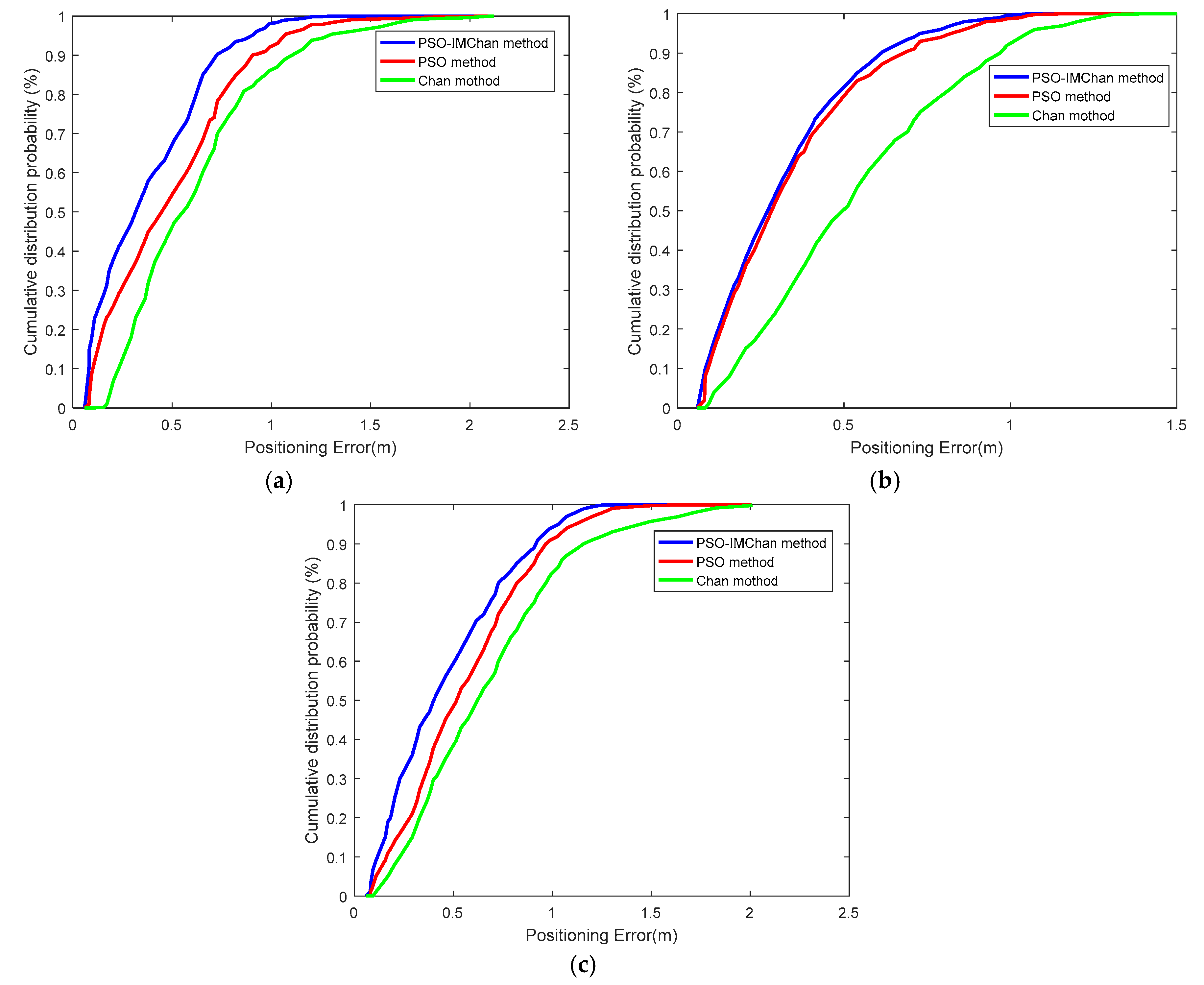
In order to better evaluate the performance of the proposed algorithm that it can effectively suppress NLOS interference, the positioning error was calculated by comparing the actual position and the estimated position of text points. Each position was tested 10 times to avoid the effect of random noise factors. To demonstrate the positioning error more clearly, we randomly focus on Scenario 3, the results of the 3-D positioning and the cumulative distribution function (CDF) curves of the positioning error are shown in Figure 3 and Figure 4, respectively. In addition, Table 2 lists the statistical results of the positioning errors in different scenarios.
To show the convergence process vividly, the relationship between the fitness and iteration times can be seen in Figure 3a. At each test position, the PSO algorithm is applied to calculate the position of the target in the experiment. After 10 generations, the fitness curve of the particle gradually converges, while the coordinate of this particle is shown in Figure 3b. Figure 4 shows the statistical results of different algorithms in different directions, where the CDF of the positioning error is defined as the cumulative distribution function. For the proposed algorithm PSO-IMChan, 90% of the 3-D positioning errors are below 0.75 m, and 90% of the horizontal and the vertical error are 0.54 m and 0.7 m, respectively, which shows a good positioning performance and is feasible in the actual positioning situation. For more practical positioning algorithms based on TOA, such as method 1 and method 2. Figure 5 shows the histogram of the positioning error in Scenario 3.
As we can see from the Figure 3 and Figure 4, it can be intuitively seen that the estimation of the proposed PSO-IMChan method is closer to the real position than those of the other two methods. As indicated by the CDF curves of the positioning error in Figure 4a, most of the 3-D positioning errors based on the PSO-IMChan method in Scenario 3 are within 0.75 m. However, from the positioning errors in Figure 5c, most of the 3-D positioning errors based on the PSO-IMChan method in Scenario 3 are within 0.65 m.
The positioning errors in different scenarios of the PSO method, Chan method and other methods are also shown in Table 2. From Table 2, it is observed that the positioning error of the proposed algorithms is less than the positioning error of Chan and PSO in several different conditions. In addition, in Scenario 3, the mean error of the proposed algorithm is 41.93% less than that of the method without the PSO optimization (the Chan method). The maximum reduced error of the proposed algorithm is 39.71% less than that of the Chan method. The minimum reduced error of the proposed algorithm is 72.82% that of the Chan method. Furthermore, the result of Scenario 3 is much better than that of other Scenarios.
4.3. Resistance Against Noise of the Algorithm
A reliable algorithm should resist the increment of the noise level (noise obeys the Gaussian distribution). We study this feature of Chan, PSO, PSO-IMChan, and other algorithms, as well as their capability in NLOS mitigation. We still focus on Scenario 3, which considers 20 stations to be employed for localization. The performance of different methods under different NLOS errors is shown in Figure 6.
From Figure 6, performance of the aforementioned algorithms are compared in terms of RMSE, when the NLOS error is small, the positioning performance of the four algorithms (PSO-IMChan, PSO method, Chan method, and WLS method) is almost the same. However, with the increase of NLOS error, the PSO method, Chan method, and WLS method cannot provide desirable performance in the presence of NLOS and demonstrates the worst accuracy. Furthermore, the localization performance of the proposed method (PSO-IMChan) is superior to that of the Chan, PSO, and other methods. This fact reflects that the proposed method can suppress the error of the NLOS effectively.
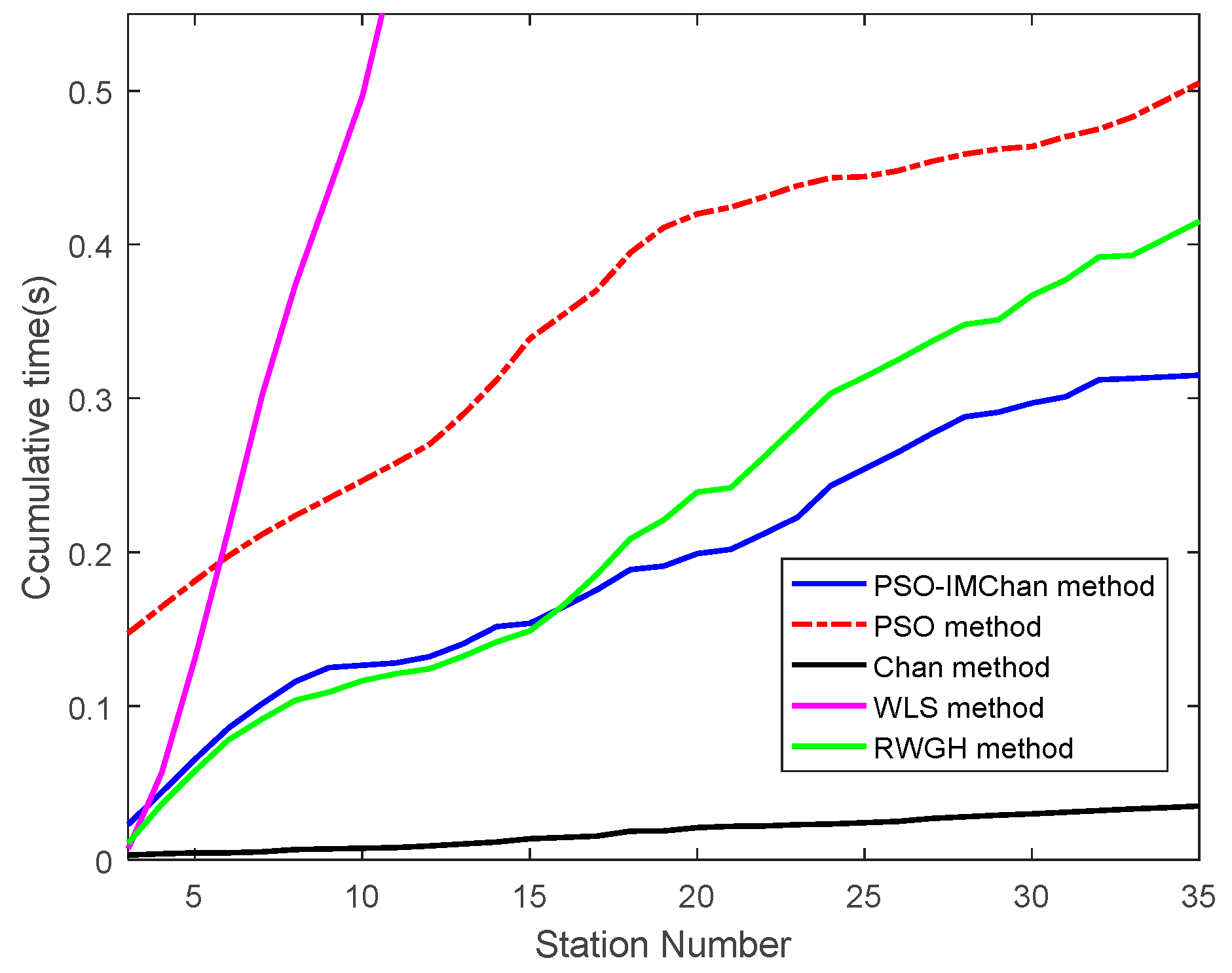
4.4. Time Complexity
It is important for an algorithm to evaluate the time complexity over a different number of positioning stations. We conduct the experiment to find out the ability of PSO, Chan, PSO-IMChan and other algorithms to deal with more positioning stations. In the section, we increase the number of stations from 3 to 35, and Figure 7 indicates the time consumption of the PSO, Chan, PSO-IMChan WLS, and RWGH methods on an Intel Core i7 3.6 GHz CPU notebook.
In Figure 7, Method 1 almost needs a calculation time in an exponential relation with the number of stations, which limits the operability of the WLS method for more BS. The Chan method requires very little computation time, but the positioning accuracy cannot meet the actual demand. Furthermore, the RWGH method and PSO-IMChan algorithms both have acceptable time complexity, however, the PSO-IMChan algorithms requires less computing time. The fact indicates that the proposed method still has high computational efficiency and lower complexity when dealing with large-scale base station positioning problems.
4.5. Analysis and Discussion
As we know, most WLAN positioning uses a fingerprint [30] matching method, but it is highly environment dependent, while the collection of a fingerprint library is difficult. Other feed-forward neural network (FNN) positioning algorithms [31,32] need to train the network parameters in advance, which take a great deal of time and a large amount of computation. Different from the methods in [18,26,27,28,29,32], in the non-ideal environment of measurement error of TOA without a Gaussian distribution, the performance of the Chan positioning algorithm is limited due to the large initial solution error. However, the PSO is a powerful population approach to solve the global optimization problems. Therefore, we use PSO to estimate the initial location of the target. On the other hand, the improved Chan algorithm based on the weighted least squares (WLS) method has some advantages, such as high calculation efficiency, simple calculation and smaller positioning error (it can reach the Cramer-Rao lower bound). Therefore, based on the initial solution of the target, we employ the improved Chan algorithm to calculate the target solution again and obtain the final exact location of the unknown target. The experimental results show that the algorithm can provide desirable accuracy while maintaining high computational efficiency in the increment of base stations and has an acceptable resistance against noise, as shown in Figure 6 and Figure 7.
5. Conclusions
Aiming to achieve a better result of positioning accuracy based on TOA technology, while increasing the practicability and simplicity of the algorithm, an improved 3D indoor positioning method using the PSO and the improved Chan algorithm have been proposed in this paper. In our system, firstly, unlike previous work, instead of identifying the NLOS BS, we transform the positioning problem into a global optimization problem and use the PSO algorithm to obtain the initial solution of the target position, which can effectively eliminate the NLOS error. Then, based on the initial solution, the Chan algorithm performs iterative computation quickly to obtain the exact solution of the target position. By experiment, we prove that the proposed method has a high positioning accuracy and good practicability, which reflects as the lower complexity and high efficiency of our algorithm. In the future, we will deploy wireless communication base stations to indoor environments, and transplant the proposed algorithm to the CPU terminal to evaluate the performance of the proposed positioning system in the ubiquitous computing environments.
Author Contributions
S.C. constructed the model and the algorithm. C.W. wrote the manuscript. Z.S. and F.W. provide the instructions and assistance during the design. All authors provide assistance in the revision of this manuscript. All authors have read and approved the final manuscript.
Funding
This research was funded by Key Program of State Commission of Science Technology of China, grant number (No. 18511101600); by the National Science Fund for Young Scholars, grant number (No. 61701296); and by the Innovation Project of Shanghai University of Engineering Science, grant number (No. 17KY0202).
Acknowledgments
This study was supported in part by Key Program of State Commission of Science Technology of China (No. 18511101600), by the National Science Fund for Young Scholars (No. 61701296), and by the Innovation Project of Shanghai University of Engineering Science (No. 17KY0202). The funder (Zhicai Shi) was involved in the manuscript writing, editing, and approval.
Conflicts of Interest
The authors declare no conflict of interest.
References
- Wang, C.Z.; Wu, F.; Shi, Z.; Zhang, D.S. Indoor positioning technique by combining RFID and particle swarm optimization-based back propagation neural network. Opt. Int. J. Light Electron Opt. 2016, 127, 6839–6849. [Google Scholar] [CrossRef]
- Xu, E.; Ding, Z.; Dasgupta, S. Source localization in wireless sensor networks from signal time-of-arrival measurements. IEEE Trans. Signal Process 2011, 59, 2887–2897. [Google Scholar] [CrossRef]
- Luo, M.; Chen, X.; Cao, S.; Zhang, X. Two new shrinking-circle methods for source localization based on TDoA measurements. Sensors 2018, 18, 1274. [Google Scholar] [CrossRef] [PubMed]
- Liu, H.; Darabi, H.; Banerjee, P.; Liu, J. Survey of wireless indoor positioning techniques and systems. IEEE Trans. Syst. Man Cybern. Part C 2007, 37, 1067–1080. [Google Scholar] [CrossRef]
- Güvenç, İ.; Chong, C.C. A survey on TOA based wireless localization and NLOS mitigation techniques. IEEE Commun. Surv. Tutor. 2009, 11, 107–124. [Google Scholar] [CrossRef]
- Kegen, Y.; Jay, G.Y. Statistical NLOS identification based on AOA, TOA and signal strength. IEEE Trans. Veh. Technol. 2009, 58, 274–286. [Google Scholar]
- Bouet, M.; Pujolle, G. A range-free 3-D localization method for RFID tags based on virtual landmarks. In Proceedings of the IEEE 19th International Symposium on Personal, Indoor and Mobile Radio Communications, Cannes, France, 15–18 September 2008. [Google Scholar]
- Wang, C.; Shi, Z.; Wu, F. An improved particle swarm optimization-based feed-forward neural network combined with RFID sensors to indoor localization. Information 2017, 8, 9. [Google Scholar] [CrossRef]
- Wang, P.; He, J.; Xu, L.; Wu, Y.; Xu, C.; Zhang, X. Characteristic modeling of TOA ranging error in rotating anchor-based relative positioning. IEEE Sens. J. 2017, 17, 7945–7953. [Google Scholar] [CrossRef]
- Kietlinski-Zaleski, J.; Yamazato, T.; Katayama, M. Experimental validation of TOA UWB positioning with two receivers using known indoor features. Position Location Navig. Symp. 2010, 37, 505–509. [Google Scholar]
- Makki, A.; Siddig, A.; Bleakley, C.J. Robust high resolution time of arrival estimation for indoor WLAN ranging. IEEE Trans. Instrum. Meas. 2017, 66, 2703–2710. [Google Scholar] [CrossRef]
- Zhang, J.W.; Yu, C.L.; Tang, B.; Ji, Y.Y. Chan location algorithm application in 3-dimension space location. In Proceedings of the 2008 ISECS International Colloquium on Computing, Communication, Control, and Management, Guangzhou, China, 4–5 August 2008; pp. 622–625. [Google Scholar]
- He, Z.; Ma, Y.; Tafazolli, R. Improved high resolution TOA estimation for OFDM-WLAN based indoor ranging. IEEE Wirel. Commun. Lett. 2013, 2, 163–166. [Google Scholar] [CrossRef]
- Wylie, M.P.; Holtzman, J. The non-line of sight problem in mobile location estimation. In Proceedings of the 5th International Conference on Universal Personal Communications, Cambridge, MA, USA, 2 October 1996; pp. 827–831. [Google Scholar]
- Luo, J.; Shukla, H.V.; Hubaux, J.P. Non-interactive location surveying for sensor networks with mobility-differentiated TOA. In Proceedings of the 25th IEEE INFOCOM, Barcelona, Spain, 23–29 April 2006; pp. 1–12. [Google Scholar]
- Riba, J.; Urruela, A. A non-line-of-sight mitigation technique based on ML-detection. In Proceedings of the 2004 IEEE International Conference on Acoustics, Speech, and Signal Processing, Montreal, QC, Canada, 17–21 May 2004; pp. 153–156. [Google Scholar]
- Chang, X.; Ye, S.; Jiang, Y.; Guan, T.; Wang, J. Three-dimensional positioning of wireless communication base station. In Proceedings of the 2017 IEEE 2nd Advanced Information Technology, Electronic and Automation Control Conference, Chongqing, China, 25–26 March 2017. [Google Scholar]
- Chen, P.C. A non-line-of-sight error mitigation algorithm in location estimation. In Proceedings of the 1999 IEEE Wireless Communications and Networking Conference (Cat. No. 99TH8466), New Orleans, LA, USA, 21–24 September 1999; pp. 316–320. [Google Scholar]
- Abolfathi, A.; Behnia, F.; Marvasti, F. NLOS mitigation using sparsity feature and iterative methods. arXiv, 2018; arXiv:1803.06838. [Google Scholar]
- Miura, S.; Kamijo, S. GPS error correction by multipath adaptation. Int. J. Intell. Transp. Syst. Res. 2015, 13, 1–8. [Google Scholar] [CrossRef]
- Suzuki, T.; Kitamura, M.; Amano, Y.; Hashizume, T. High-accuracy GPS and GLONASS positioning by multipath mitigation using omnidirectional infrared camera. In Proceedings of the 2011 IEEE International Conference on Robotics and Automation (ICRA 2011), Shanghai, China, 9–13 May 2011; pp. 311–316. [Google Scholar]
- Al-Jazzar, S.; Caffery, J.; You, H.R. A scattering model based approach to NLOS mitigation in TOA location systems. In Proceedings of the IEEE 55th Vehicular Technology Conference, VTC Spring 2002 (Cat. No.02CH37367), Birmingham, AL, USA, 6–9 August 2002; pp. 861–865. [Google Scholar]
- Van Laarhoven, P.J.; Aarts, E.H. Simulated annealing. In Simulated Annealing: Theory and Applications; Springer: Dordrecht, The Netherlands, 1987; pp. 1–7. [Google Scholar]
- Gopakumar, A.; Jacob, L. Localization in wireless sensor networks using particle swarm optimization. In Proceedings of the IET Conference on Wireless Mobile and Multimedia Network, Mumbai, India, 11–12 January 2008; pp. 227–230. [Google Scholar]
- Areas, I.O. A Wi-Fi indoor localization strategy using particle swarm optimization based artificial neural networks. Int. J. Distrib. Sensor Netw. 2016, 2016, 33. [Google Scholar]
- Jiang, H.; Liu, C.; Sun, X. An application of canonical decomposition to TDOA estimation for 3D wireless sensor network node localization. Przeglad Elektrotech. 2012, 88, 92–95. [Google Scholar]
- Chen, X.; Zhang, B. 3D DV–hop localisation scheme based on particle swarm optimisation in wireless sensor networks. Int. J. Sensor Netw. 2014, 16, 100–105. [Google Scholar] [CrossRef]
- Zhang, J.W.; Yu, C.L.; Ji, Y.Y. The Performance Analysis of Chan Location Algorithm in Cellular Network. In Proceedings of the 2009 WRI World Congress on Computer Science and Information Engineering (CSIE 2009), Los Angeles, CA, USA, 31 March–2 April 2009; pp. 339–343. [Google Scholar]
- Einemo, M.; So, H.C. Weighted least squares algorithm for target localization in distributed MIMO radar. Signal Process 2015, 115, 144–150. [Google Scholar] [CrossRef]
- Oh, J.; Kim, J. Adaptive k-nearest neighbour algorithm for WiFi fingerprint positioning. ICT Express 2018, 4, 91–94. [Google Scholar] [CrossRef]
- Kuo, R.J.; Chang, J.W. Intelligent RFID positioning system through immune-based feed-forward neural network. J. Intell. Manuf. 2015, 26, 755–767. [Google Scholar] [CrossRef]
- Pahlavani, P.; Gholami, A.; Azimi, S. An indoor positioning technique based on a feed-forward artificial neural network using levenberg-marquardt learning method. ISPRS Int. Arch. Photogramm. Remote Sens. Spat. Inf. Sci. 2017, 435–440. [Google Scholar] [CrossRef]
Figure 1.
The framework of the PSO-IMChan based on the positioning system.
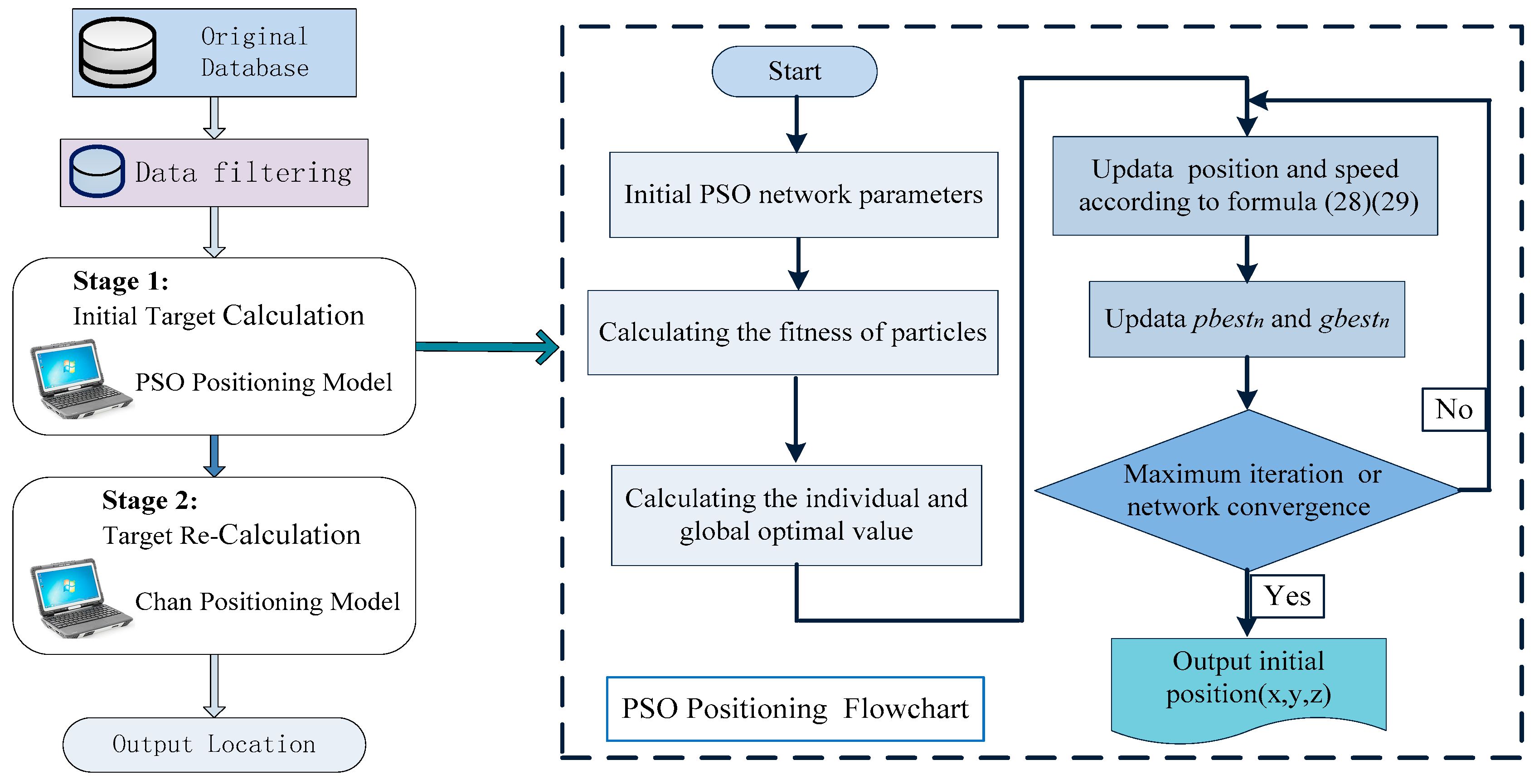
Figure 2.
The 3-D positioning scenarios of the four experiments.
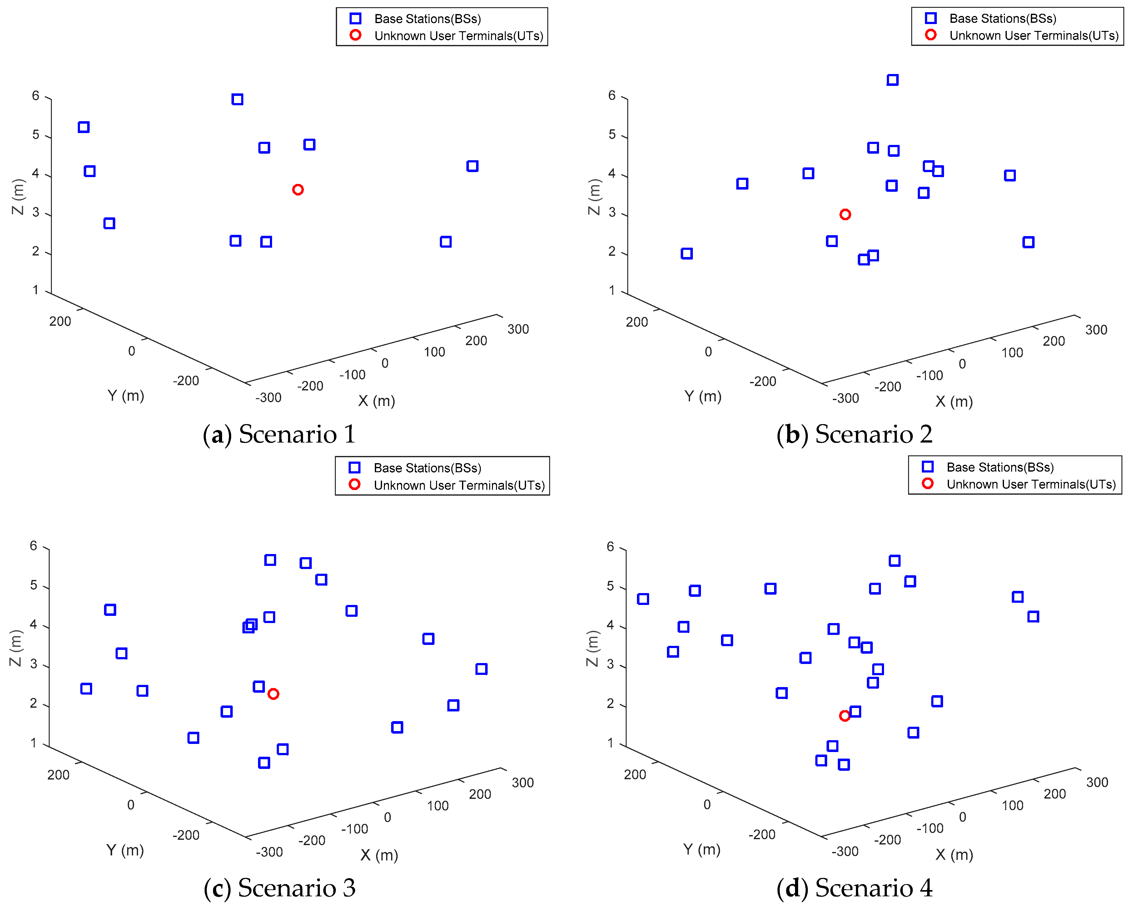
Figure 3.
The distribution of the real position and its estimated 3-D position. (a) The relationship between iteration times and the best fitness of the particle swarm; (b) positioning results based on PSO model; (c) initial calculation results based on the Chan algorithm; (d) re-calculation results based on the Chan algorithm; (e) initial calculation results based on the PSO algorithm; and (f) re-calculation results based on the proposed PSO-IMChan algorithm.
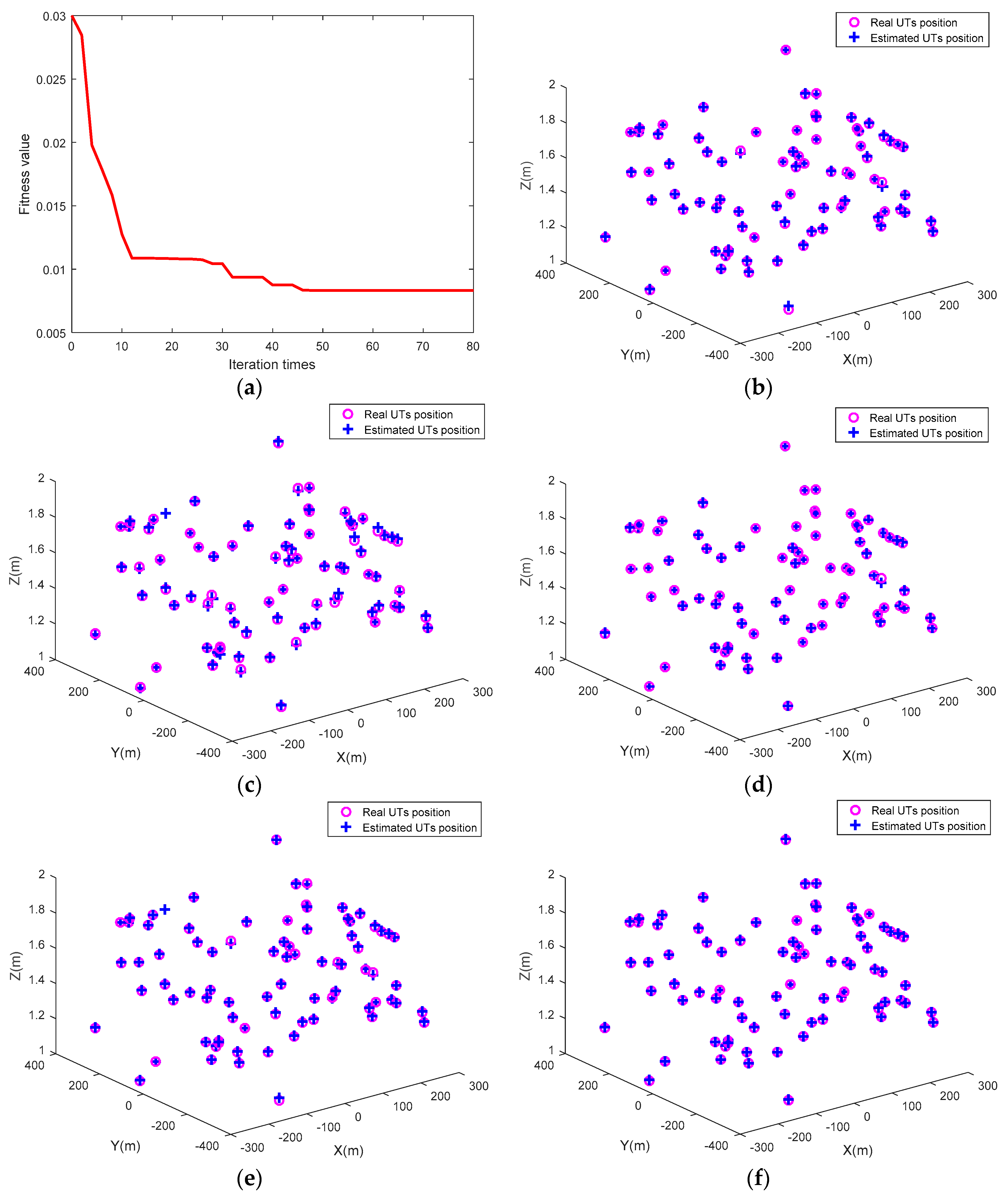
Figure 4.
The CDF curves of positioning error. (a) 3-D positioning CDF; (b) horizon positioning error CDF; and (c) vertical positioning error CDF.
Figure 4.
The CDF curves of positioning error. (a) 3-D positioning CDF; (b) horizon positioning error CDF; and (c) vertical positioning error CDF.

Figure 5.
Histogram of the positioning error in the Scenarios 3. (a) PSO method; (b) Chan method; (c) PSO-IMChan method; (d) WLS method; and (e) RWGH method.
Figure 5.
Histogram of the positioning error in the Scenarios 3. (a) PSO method; (b) Chan method; (c) PSO-IMChan method; (d) WLS method; and (e) RWGH method.

Figure 6.
The performance of different methods under different NLOS noise standard deviation.
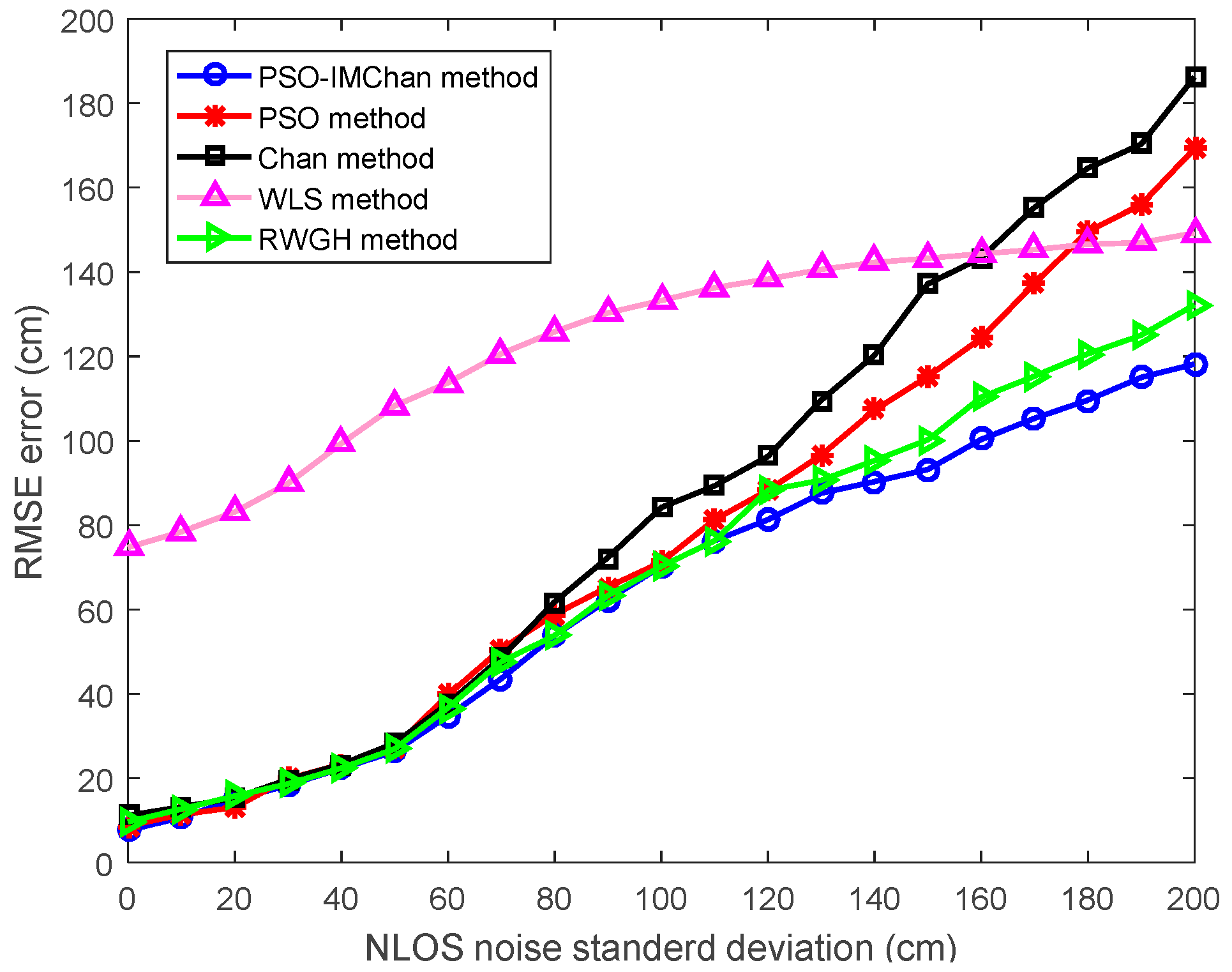
Figure 7.
Required time for different methods versus the number of BS.

Table 1.
The parameters (Pars.) setting for PSO algorithms.
| Pars. | Inertia Weight | Iteration Number | Population Size | Learning Factor | Range of Velocity and Position |
|---|---|---|---|---|---|
| 80 | 50 | [−1, 1] |
Table 2.
The positioning error of different scenarios (m).
| Positioning Error | PSO | Chan | PSO-IMChan | WLS | RWGH | |
|---|---|---|---|---|---|---|
| Scenario 1 | Min | 0.1686 | 0.5087 | 0.1684 | 0.1133 | 0.2928 |
| Max | 2.0511 | 2.2832 | 1.6282 | 1.5454 | 1.7821 | |
| Mean | 1.1843 | 1.4827 | 0.9053 | 0.8911 | 1.1104 | |
| Std. | 0.9249 | 1.1015 | 0.7185 | 0.7102 | 0.9033 | |
| Scenario 2 | Min | 0.1664 | 0.3424 | 0.0891 | 0.0779 | 0.2999 |
| Max | 1.9279 | 1.9867 | 1.4129 | 1.5444 | 1.5118 | |
| Mean | 0.9114 | 1.3428 | 0.7334 | 0.8812 | 0.8823 | |
| Std. | 0.7744 | 0.9351 | 0.5579 | 0.5688 | 0.5518 | |
| Scenario 3 | Min | 0.0805 | 0.2057 | 0.0559 | 0.0483 | 0.1922 |
| Max | 1.8464 | 2.0888 | 1.2594 | 1.5512 | 1.2046 | |
| Mean | 0.9025 | 1.1146 | 0.6473 | 0.7684 | 0.8708 | |
| Std. | 0.7199 | 0.8593 | 0.4372 | 0.5677 | 0.4021 | |
| Scenario 4 | Min | 0.0685 | 0.1143 | 0.0547 | 0.0588 | 0.1818 |
| Max | 1.6886 | 1.8817 | 1.0114 | 1.6444 | 1.2233 | |
| Mean | 0.8692 | 1.0119 | 0.5087 | 0.6659 | 0.5991 | |
| Std. | 0.6328 | 0.7392 | 0.4130 | 0.5633 | 0.4144 | |
© 2018 by the authors. Licensee MDPI, Basel, Switzerland. This article is an open access article distributed under the terms and conditions of the Creative Commons Attribution (CC BY) license (http://creativecommons.org/licenses/by/4.0/).
Share and Cite
MDPI and ACS Style
Chen, S.; Shi, Z.; Wu, F.; Wang, C.; Liu, J.; Chen, J. Improved 3-D Indoor Positioning Based on Particle Swarm Optimization and the Chan Method. Information 2018, 9, 208. https://doi.org/10.3390/info9090208
AMA Style
Chen S, Shi Z, Wu F, Wang C, Liu J, Chen J. Improved 3-D Indoor Positioning Based on Particle Swarm Optimization and the Chan Method. Information. 2018; 9(9):208. https://doi.org/10.3390/info9090208
Chicago/Turabian StyleChen, Shanshan, Zhicai Shi, Fei Wu, Changzhi Wang, Jin Liu, and Jiwei Chen. 2018. "Improved 3-D Indoor Positioning Based on Particle Swarm Optimization and the Chan Method" Information 9, no. 9: 208. https://doi.org/10.3390/info9090208
Note that from the first issue of 2016, this journal uses article numbers instead of page numbers. See further details here.