Article

Genetic Algorithm with an Improved Initial Population Technique for Automatic Clustering of Low-Dimensional Data

1
School of Information and Engineering, Sichuan Tourism University, Chengdu 610100, China
2
Key Lab of Earth Exploration & Information Techniques of Ministry Education, Chengdu University of Technology, Chengdu 610059, China
3
School of Mathematics and Computer Science, Aba Teachers University, Wenchuan 623002, China
4
School of Computer Science, Chengdu University of Information Technology, Chengdu 610225, China
*
Author to whom correspondence should be addressed.
Information 2018, 9(4), 101; https://doi.org/10.3390/info9040101
Submission received: 1 March 2018 / Revised: 17 April 2018 / Accepted: 19 April 2018 / Published: 21 April 2018

Abstract

:
K-means clustering is an important and popular technique in data mining. Unfortunately, for any given dataset (not knowledge-base), it is very difficult for a user to estimate the proper number of clusters in advance, and it also has the tendency of trapping in local optimum when the initial seeds are randomly chosen. The genetic algorithms (GAs) are usually used to determine the number of clusters automatically and to capture an optimal solution as the initial seeds of K-means clustering or K-means clustering results. However, they typically choose the genes of chromosomes randomly, which results in poor clustering results, whereas a generally selected initial population can improve the final clustering results. Hence, some GA-based techniques carefully select a high-quality initial population with a high complexity. This paper proposed an adaptive GA (AGA) with an improved initial population for K-means clustering (SeedClust). In SeedClust, which is an improved density estimation method and the improved K-means++ are presented to capture higher quality initial seeds and generate the initial population with low complexity, and the adaptive crossover and mutation probability is designed and is then used for premature convergence and to maintain the population diversity, respectively, which can automatically determine the proper number of clusters and capture an improved initial solution. Finally, the best chromosomes (centers) are obtained and are then fed into the K-means as initial seeds to generate even higher quality clustering results by allowing the initial seeds to readjust as needed. Experimental results based on low-dimensional taxi GPS (Global Position System) data sets demonstrate that SeedClust has a higher performance and effectiveness.

1. Introduction

Data clustering is an important and well-known technique in the area of unsupervised machine learning. It is used for identifying similar records in one cluster and dissimilar records in different clusters [1,2,3,4,5]. Moreover, cluster analysis is a statistical multivariate analysis technique in clustering area, which has a wide range of application fields, including social network analysis, pattern recognition, geographic information science, and knowledge discovery. There are many clustering algorithms, which have been roughly categorized into six classes [1]: partition-based (e.g., K-means), density-based (e.g., DBSCAN (Density-Based Spatial Clustering of Applications with Noise) and OPTICS (Ordering Points to Identify the Clustering Structure), model-based (e.g., Gaussian model and regression model), hierarchical-based (e.g., RIRCH (Balanced Iterative Reducing and Clustering using Hierarchies), CURE (Clustering Using REpresentatives), FocalPoint Clustering [6], Agglomerative hierarchical clustering [7]), graph-based (e.g., spectral clustering), and grid-based (e.g., STING (Statistical Information Grid), flexible grid-clustering [8], and grid-growing clustering [9]), out of which partition-based are undoubtedly the most widely and popular techniques for clustering. Therefore, in this paper, we mainly focus on the partition-based clustering algorithm. Typically, K-means is a commonly-used clustering technique perhaps because of its simplicity and effectiveness. However, K-means also has a number of well-known drawbacks that usually obtains poor results where clusters have different sizes and shapes. These drawbacks mainly include requiring a user to provide the number of clusters K as an input [2,10], which is generally very sensitive to the quality of the initial seeds, and easily produces poor quality results due to the poor quality of the initial seeds [10,11]. Existing techniques have been proposed, for finding higher-quality initial seeds than the initial seeds K-means selects randomly [3,4,12,13]. For example, work in [3] presented an efficient K-means clustering filtering algorithm using density-based initial seeds, which improved the performance of the K-means filtering method by locating the seed points at dense areas of the data set and well separated. The authors in [4] presented fast density clustering strategies based on K-means, which could enhance the scalability of the fast search and find the density peaks, while maintaining its clustering results as far as possible. Meanwhile, in initial seeds processing, K-means++ [14] can be used to handle the sensitiveness of the initial seeds of K-means [15], and its complexity is also very low. However, when the distances are computed between the data points, the K-means++ algorithm does not know the distribution of the data points, resulting in seeds that are uneven in distribution and needs repeated calculating.
Additionally, with K-means, it is difficult to capture the global optimal solution results in producing poor clustering results [10,16,17]. In order to strengthen the performance and the efficiency of the K-means algorithm, several GAs with K-means have been proposed in the past years [18,19,20]. These genetic algorithms (GA)-based clustering algorithms can produce better clustering results than simple K-means or basic GA clustering. Typically, the use of GAs with K-means can also help to avoid the local minima issues of K-means [10,18,19,20,21], and a GA-based clustering technique does not require a user input on the number of clusters [21] using the adaptive operation of GAs. For example, AGCUK (Automatic genetic clustering for unknown K) [20] presented an automatic genetic clustering algorithm that could automatically find the number of clusters. GAGR (Genetic algorithm with gene rearrangement) [18] proposed a GA-based K-means clustering algorithm with gene rearrangement in order to capture the global optimum. GGA (Group genetic algorithm) [19] in the initial population developed a GA-based clustering algorithm with a new grouping method. TGGA (Two-stage genetic algorithm) [22] presented a two-stage genetic for automatic clustering, which can automatically determine the proper number of clusters and the proper partition from a given data set. In particular, GenClust [10] can automatically find the proper number of clusters and to find the right genes through an initial population approach. However, these GAs with K-means can lose population diversity due to global optimal problems, and weak exploitation capabilities in each GA operation (including selection, crossover, mutation, and elitism) [21,23,24,25]. Furthermore, the gene size of the chromosomes must be equal in the AGCUK, GAGR, and TGCA. In the GGA algorithm, the number of clusters requires a user input, but gene sizes are not equal. Nevertheless, these have a high time complexity; for instance, the time complexity of GenClust tends to be high and reaches O ( n 2 ) and the time complexity of TGCA is more than O ( n 2 ) . Surprisingly, the time complexity of other clustering techniques based on GA reached O ( n 3 ) , including HC (High throughput biological data clustering) [26] and ACAD (Automatic clustering inspired by ant dynamics) [27], where n is the number of data points.
GenClust presents a set of systematically-selected chromosomes in the initial population for capturing clusters of different sizes and shapes without requiring user input on the number K and specifying the number of genes; moreover, it has improved gene and chromosome operations of AGCUK [20]. In addition, GenClust also proposes a novel gene rearrangement technique that can handle chromosomes with different sizes, which has improved the crossover operation issue of AGCUK (which does not rearrange the genes before the crossover operation) and the same gene size issue of GAGR [18]. However, GenClust can handle two chromosomes participating in a crossover operation without considering the relationship between two participating chromosomes, and it may then end up having useless offspring chromosomes that are participating in the crossover operation. Meanwhile, GenClust can also improve the local minima issue of K-means using GA. However, the complexity of the initial population of GenClust has high complexity with O ( n 2 ) .
In this paper, the main works of our improved clustering technique, called SeedClust, which combines AGA with an improved initial population for K-means clustering. Part of our novel clustering technique includes an improved density estimation and K-means++, which are used to generate the initial population and initial seeds without requiring the user to input the number of clusters and process the initial seeds as well as handle the different size and shape of the genes. When compared to GenClust, the advantage of SeedClust on the initial population is that it is simple and fast without suffering from the impact of the higher complexity. Therefore, SeedClust may improve the sensitivity of the initial seeds and the use of the selected initial population in the AGA. The presented SeedClust can maintain population diversity and premature convergence.
Therefore, the main contributions of the presented SeedClust are described, as follows:
On one hand, our technique used taxi GPS data encoding genes to realize chromosome representations in order to find urban traffic information and to understand the population migration distribution (see Section 3.1), then an improved density estimation method is presented to choose chromosomes in the initial population for capturing the number of clusters, which are chosen between [ 2 , n ] [10,20] with a low complexity. In Section 3, we present an analysis to describe the advantage of the initial population in the AGA. Unlike some existing GA-based clustering algorithms, such as AGCUK [20], GAGR [18], and GGA [19], which select the initial genes randomly, according to [10], the initial technique of GenClust is superior to AGCUK, GAGR, and GGA. Our proposed SeedClust included both a set of densities and a threshold in the initial population, where densities are used to capture the number of clusters, and threshold T is used to control the size of the initial genes for each chromosome. Another goal of the paper, the inverse of SSE (sum of quadratic errors) are employed as fitness functions of AGA.
On the other hand, to verify the performance and the effectiveness of SeedClust, we compared SeedClust with GenClust [10], GAK [28], GA-clustering [17], and K-means on four low-dimensional taxi GPS data sets [29], which consisted of Aracaju (Brazil), Beijing (China), New York (USA), and San Francisco (USA). We also compared four cluster evaluation criteria: SSE, DBI (Davis-Bouldin Index) [30], PBM-index [31], and silhouette coefficient (SC) [19]. In addition, a complexity of SeedClust analysis is presented in Section 2.5, which indicated that the complexity of SeedClust is lower.
Unlike most of the existing GA-based clustering techniques, such as [10,18,19,20], SeedClust can handle the number of clusters and initial seeds by densities in the initial population, maintain the population diversity by adaptive crossover and mutation probabilities, and can also avoid getting stuck in a local optimum. Finally, SeedClust can obtain a set of optimization seeds (best chromosome) for a given data set, which are applied to the K-means clustering. Therefore, SeedClust has three main steps: firstly, according to the density-based and improved K-means++ method, the initial population is produced; secondly, the determination of the best chromosome (the seeds and the number of clusters) is obtained through the AGA; and thirdly, the use of the best chromosome as the initial seeds of the K-means to finally generate high-quality clustering results.
Therefore, the main contributions of the study can be summarized as follows:
  • The selection of the initial population combining the improved K-means++ and density estimation with a low complexity (see Section 2.2).
  • The AGA is used to prevent the SeedClust from getting stuck at a local optimal and to maintain population diversity (see Section 2.4).
  • The SeedClust worked on low-dimensional taxi GPS data sets (see Section 3.1).
The remainder of the paper is organized as follows: Section 2 describes our proposed SeedClust algorithm. Experimental results are presented in Section 3. Finally, Section 4 offers conclusions and future work.

2. The Proposed SeedClust Clustering Algorithm

This section includes some steps as follows: (1) The four real-world taxi GPS data (location information) are used to encode each chromosome; (2) The improved initial population technique is proposed using density and an improved K-means++ in Section 2.2, and the best chromosome is obtained to use K-means clustering, which can also be used to obtain the number of clusters and the initial seeds of the K-means clustering operations; (3) The reciprocal of the SSE is employed as a fitness function with the aim to capture the maximum value of genetic operation; (4) A gene rearrangement technique based on cosine, adaptive probabilities of crossover and mutation, and elitist operation, is employed to execute the genetic optimization in term of the work [32]; and, (5) The complexity of the SeedClust algorithm is analyzed in Section 2.5, as shown in Figure 1.

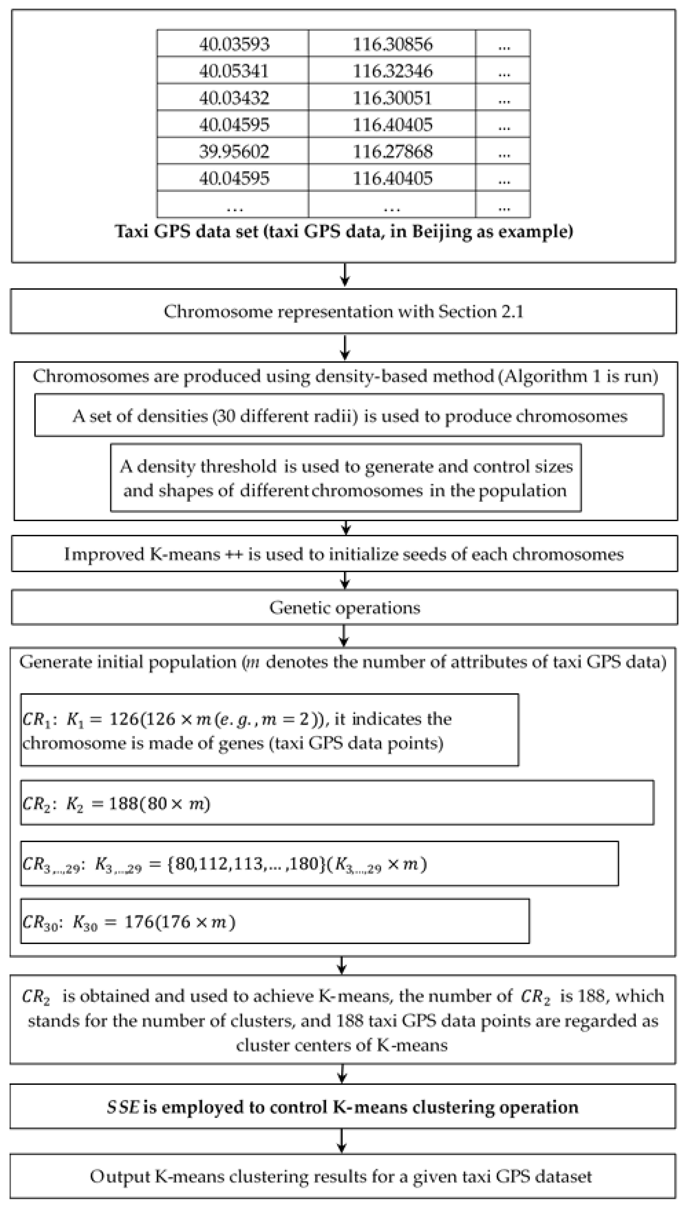
2.1. Chromosome Representation

In this paper, a given data set is utilized to describe the chromosome in this paper, furthermore, a density-based method is proposed to use the initial selection of chromosomes and an improved K-means++ is also used to select the initial seeds (see Section 2.2). Each seed of the cluster is represented by the chromosome in the same way as the SeedClust algorithm. In addition, the number of genes of a chromosome must be chosen and be controlled between [ 2 , n ] , where n is the number of taxi GPS data points. The genes of each chromosome has a different size and shape, and can be used as input for the K-means clustering (the best chromosome is chosen from the final population and is then used to handle the K-means clustering), which can handle all kinds of data sets as the data sets can generate chromosomes, if SeedClust is used to achieve the clustering of the high dimension data sets, a multidimensional Euclidean distance equation can be employed to replace the two-dimensional Euclidean [33]; moreover, when each seed no longer changes in each cluster, the corresponding seed has to be determined. Therefore, chromosome representation is described by real-world taxi GPS data points, which can be defined by C R ( G i 1 , G i 2 , , G i K ) , or C R ( S i 1 , S i 2 , , S i K ) . Note that a gene is regarded as a seed, in other words, a real data point is regarded as a seed, a cluster is regarded as a chromosome, and a chromosome consists of seeds in clustering algorithms [10,21], in clustering processing, where CR, G, S, K, i denote the chromosomes, genes, seeds, the number of seeds (or the number of genes of chromosome, [ 2 K n ] ), and the number of data points each cluster, respectively. Next, the length of the chromosomes is K i × m , where K i stands for the number of clusters of the ith chromosome and m denotes the number of data attributes (m dimensions) and the initial population produced processing is described in Section 2.2.1. Therefore, the chromosomes are made up of real data representing the seeds (cluster centers) in the initial population, and are then used to achieve genetic operation.

2.2. Population Initialization

Population has been verified by experiments where the appropriate initial seeds greatly affect the quality of clustering [34,35]. The adverse effects of improper population include slower convergence, and a higher chance of trapping in the local minima [36]. Fortunately, all of these drawbacks can be remedied and enhanced by using many initialization techniques. In general, there are five categories for clustering initialization population methods: random sampling selection methods [18], distance optimization methods, density estimation methods [10], attribute feature methods, and noise selection methods [20]. However, for these initialization approaches, there are more or less shortcomings, i.e., the seeds are chosen randomly using random sampling selection methods, which only works well when the number of clusters is small and the chances are good that at least one random initialization is close to a good solution; in the density-based methods, when the single density estimation radius is used to initialize, it is not efficient for a large number of data sets, which results in causing an uneven distribution and spend time-consuming; sensitivity to the threshold is a prominent drawback for the distance-based initial method; for the noise-based initial method, it is sensitive to the set noise rate; attribute feature methods choose initial seeds in light of the attribute features of data, however, it is difficult to capture the data features of the attribute. The authors in [11] investigated some of the most popular initialization methods that were developed for K-means clustering operation, and some of the commonly used initial methods with an emphasis on their time complexity are reviewed, which included linear time-complexity (e.g., K-means++ [14]), quadratic-complexity, and other methods. Authors in [10] presented a density-based initial population selection technique and the use of the selected initial population in a GA. In [37], they proposed a new initialization method that is based on the frequency of attribute values for categorical data clustering, which considered the distance between objects and the density of the object. In this paper, a density-based method is proposed to produce the initialization population for genetic operation, and an improved K-means++ method is presented to generate initial seeds.

2.2.1. Initial Operation Using a Density Method

Many density-based methods have been widely applied in clustering research [10,38,39]. Therefore, in this paper, a density-based method is employed to initialize the population for GA as it directly divides the taxi GPS data densities reachable from different points into chromosomes, and then produces chromosomes with different sizes and shapes. In the SeedClust algorithm, according to the existing initialization technique in [10], the given radius set is placed in data sets to draw some circles (density distribution), count the number of data points in each circle, and then find the densities according to the number of data points in each circle, so all of the data points within the radii are removed from the data set. Furthermore, it is meaningful to find an appropriate method to estimate the density using a group of existing density radii r ( r x = { r 1 , r 2 , , r NIND } ) parameter (r = [0.0001, 0.0005, 0.001, 0.002, 0.003, 0.004, 0.005, 0.006, 0.007, 0.008, 0.009, 0.01, 0.02, 0.03, 0.04, 0.05, 0.06, 0.07, 0.08, 0.09, 0.1, 0.11, 0.12, 0.13, 0.14, 0.15, 0.16, 0.17, 0.18, 0.2]; we mean an r x value that can generate a number of clusters or constitute a chromosome, for example, a set of radii can be equal to 30). The above operations are repeated until all of the data points are assigned by giving densities, which indicates that 30 chromosomes have be generated for the initial population.
In the processing, the density-based method first needs to normalize a data set using the formula V norm = ( V V min ) / ( V max V min ) , where V denotes the attribute values of taxi GPS data points; the maximum and minimum distance between the taxi GPS data are 1 and 0, respectively; this means there are 30 different r x values ranging between 0 and 1, let r x values be effective for taxi GPS dataset when the density-based method is used to produce chromosomes. For instance, let m = 2, K i = 3 then a set of given GPS (Global Position System) location data points {(–10.92435261,–37.04431889), (–10.93428983,–37.0499316), (–10.92635717,–37.10253)}, then V norm = {(1, 1), (0, 0.90358009), (0.79827758669, 0)}. Second, in order to produce a chromosome, a radius r x is chosen to calculate the density of each taxi GPS data point of the data set as follows: { G j : dist ( G i , G j ) r x , j } where dist denotes Euclidean distance (if the taxi GPS data are high dimensional data characteristics, and then a multidimensional Euclidean distance formula is employed to replace two-dimensional Euclidean [33]), which is used to calculate the distance between the normalized data points. Each data point having the highest density is then chosen as the first gene, until one gets a data point with a density greater than a user defined threshold T (e.g., T = | length ( dataset ) | / 100 ). Therefore, for a r x value, the density-based method can obtain a number of genes from a chromosome C R j , and use the different r x values to produce the different chromosomes until 30 radius values have all been applied. The density-based method is described, as follows.
When Algorithm 1 is run, the number of clusters (chromosomes) indicated have been automatically captured.
Algorithm 1. Population generation using density estimation method
Input: a given data set data,
Output: population results
Procedure:
Initial parameters
  Define a set of radius r x ;
  Define m is dimension of the given a data set;
  the normalized data V norm = { V 1 , V 2 , , V n } of the given dataset;
  the initial population matrix DM;
  threshold T;
FOR x = 1 to NIND
//NIND denotes the size of population which is defined by a user, and radius r x = r NIND .
  FOR y = 1 to n
    Compute distances dist between data points using the normalized data ( V norm );
    DM←dist ≤ POP (data, NIND, r x , V norm ,   m );
    //POP is fitness of density estimation, and the results are stored in DM.
    IF r x < T
     Generate chromosomes C R x ( x = 1 , , NIND ) ;
    ELSE
     Return and run next radius value until r x is null (WHILE loop is end);
    END IF
   END FOR
END FOR

2.2.2. Initial Seeds Using an Improved K-Means++ Method

It is well-known that high quality initial seeds can strengthen the clustering quality of the K-means clustering algorithm [11,40]. Therefore, an improved K-means++ algorithm is presented to initialize the seeds and to capture a high-quality initial population. The K-means++ algorithm is both a fast and simple way of choosing seeds for the K-means algorithm [14,41], and has low computing cost, namely, its complexity is only ( O ( log K ) . It chooses the first seed randomly and the ith ( i { 2 , 3 , , K } ) seed is chosen to be S C R with a probability of P + = D ( S ) 2 / j = 1 n D ( S j ) 2 ) , where D(S) denotes the shortest distance from a data point to the closest center we have already chosen; and, n stands for the number of data points. Meanwhile, K-means++ is a greedy algorithm, it probabilistically selects log K seeds in each round and then greedily chooses the seed that most reduces the SSE. This modification aims to avoid the unlikely event of choosing two seeds that are close to each other, another advantage of K-means++ is that it is easy to find seeds of a data set without too much consideration of the sensitiveness of the seeds. However, in a high-density data set, when K-means++ randomly selects the first seeds, this results in other seeds that cannot be evenly distributed, and the distance between the seeds are also close together, resulting in getting stuck at a local minima. We therefore presented a density-based method to improve the seed selection of K-means++.
The improved K-means++ algorithm is presented in two parts, as follows: first, in the K-means++ algorithm, we used a set of densities r x to replace randomly selection probability P + of the data points, in other words, the seeds/cluster centers of each chromosome are obtained by density estimation, which is shown in Section 2.2.1. Second, the initial population is produced in terms of seeds of each chromosome, namely, in the initial population, each chromosome consists of seeds of different sizes and shapes, which is shown in Algorithm 2. Finally, the initial population is produced. According to each given radius value, we got a chromosome and therefore, we obtained 30 chromosomes according to r x values as part of the initial population. Meanwhile, another 30 chromosomes are randomly selected in order to strengthen the diversity of the initial population, and the number of genes (clusters) of chromosomes is also randomly chosen [ 2 , n ] . As a result, 60 chromosomes are produced in the initial population. The improved K-means++ method is shown, as follows.
Algorithm 2. Initial seeds with an improved K-means++
Input: a set of densities r x and the normalized data V norm = { V 1 , V 2 , , V n }
Output: the initial population POP including initial seeds
Procedure:
Define m is dimension of the given a data set;
Compute the number of seeds K x ( x = 1 , , NIND ) of each chromosome in Algorithm.1;
FOR x = 1 to NIND
  FOR k = 1 to K x
    FOR y = 1 to n // n denotes number of the taxi GPS data points
       C R s C R x : S 1 k
// Randomly take one seed S 1 k from chromosome C R x ,
// C R s denotes chromosome of the initial seeds
       C R s k S i k : S e e d ( C R x , r x ,   K x , m )
// Take a new seed S i k in uniformly chromosome C R x ,
// choose gene G i k with density r x as probability,
// Seed denotes a function of seed selection, which is used to initialize seeds of each chromosome
// C R s k denotes chromosomes of the initial seeds in uniformly K x
    END FOR
  END FOR
  Repeat operation until x = NIND and K x seeds altogether have been taken
END FOR
FOR 1 to NIND
Randomly generate NIND chromosomes;
Randomly select seeds of each chromosome;
END FOR
  Generate an initial population (2*NIND chromosomes) including initial seeds of each chromosome

2.3. Fitness Function

The fitness function is usually used to describe a fitness value for each candidate solution in a given population. In SeedClust, a fitness function must be defined for the evaluation of the clustering in each chromosome. A good fitness function can capture a high value to a good partition solution and use a low value to bad partition. Since K-means is an unsupervised process in clustering analysis and it is very sensitive to seeds as input parameters, it is important to evaluate the result of K-means clustering. Nowadays, there are many validity indices used as fitness function to evaluate seed selection of clustering, and mainly include the Davies-Bouldin index (DBI), PBM-index, and Dunn index, and Silhouette index [10,22,31,42]. Nevertheless, the DBI gives good results for distinct groups, but is not designed to accommodate overlapping clusters; the Dunn index is useful for identifying clean clusters in given data sets containing no more than hundreds of data points; the Silhouette index is only able to identify the first choice and therefore should not be applied to data sets with sub-clusters, but can be used to evaluate clustering results; the PBM-index is usually used to identify the clustering performance, and thus is proposed as a measure of indication for the goodness/validity of a cluster solution, and is usually used to evaluate clustering results. In this paper, SSE is used as the fitness function as it is known that SSE has been utilized as a fitness function due to effective and low complexity, and is defined as
S S E = K x G i k x C R x d 2 ( C R x , S i k x ) ( x = 1 , , NIND )
where K x denotes the number of clusters in each chromosome; G i k x C R x denotes a data point in each chromosome assigned uniformly (note that a chromosome is a cluster in given data set); and, d 2 ( C R x , S i k ) is the Euclidean distance from the observed chromosome (a chromosome is defined for a vector) C R x to the seeds of the cluster K x , represented by the S i k . This measure computes the cumulative Euclidean distance of each pattern from its seed of each chromosome, and then sums those measures over each chromosome with the aim to capture the best chromosome from K x , and therefore use K-means clustering, namely, each chromosome with a different number of clusters represent different data partitions. If this SSE measure value is small, then the distances from patterns to seeds are all small and the clustering is regarded favorably. It is interesting to note that the minimum value of SSE can be equal to 0 when a chromosome only contains a data point. Therefore, the SSE-based fitness function of the chromosome for GA evolutionary is defined as the inverse of SSE.
f = 1 S S E
This SSE-based fitness function f is used to capture the maximum values of each chromosome during the evolutionary process (GA operations) and it leads to the minimization of the SSE. In other words, when the maximum values of fitness function f are captured during the GA operation process for each chromosome, it indicates that SSE can obtain minimum values, and the best chromosome is obtained by the minimum SSE values, which is finally used for K-means clustering.

2.4. Adaptive Genetic Operation

This section mainly discusses the method that is used to handle genetic operation according to [32]: (1) an improved gene rearrangement method based on cosine is employed; and, (2) adaptive probabilities of crossover and mutation are also used to prevent the convergence to a local optimum without defining the genetic parameters. The adaptive genetic operation is described, as follows.
Part 1. Initialization population
a. Population generation (see Algorithm 1): For a given data set, the density-based method is employed to estimate the number of genes of each chromosome. Namely, a set of density radii r x are defined in terms of the work in [10], and then estimate the number of genes of each chromosome according to the population size (NIND); the sizes and shapes of each chromosome have unequal length and are different in the population, and the NIND is usually defined by a user. Meanwhile, in order to enhance diversity of the initial population, NIND numbers of chromosomes are also randomly produced. Note that, a chromosome is a cluster; genes in a chromosome are the initial seeds.
b. Initial seeds (see Algorithm 2): An improved K-means++ method using density is proposed to perform initial seeds each chromosome. Namely, the density radii r x are used to replace the probability P + of K-means++, with its aim to initialize the seeds of each chromosome. However, if the density values are r x > 1 , then r x needs to be normalized to a range between 0 and 1 ([0, 1]). As a result, the seeds of each chromosome are initialized by the improved K-means++, and an initial population POP is generated.
Part 2. Adaptive genetic operation
a. Selection operation: NIND number of chromosomes P O P s from the population (2*NIND number of chromosomes) are selected according to the descending order of their fitness values. The selection operation of GAG can be described in Algorithm 3.
Algorithm 3. Selection operation algorithm of GAG
  Input: an initial population POP using Algorithm 2;
  Output: P O P s // selection operation population;
  Procedure:
  Initial parameters
  Define the number of iterations G of the adaptive genetic algorithm;
  Define m is dimension of the given a data set;
   P O P s // denotes the set of selected chromosomes, initially set to null
  / / Selection operation
  FOR 1 to 2*NIND
     P O P s S o r t ( N I N D ) : F i t F ( P O P , 2 * N I N D , f , m )
  // FitF is used to compute fitness values each chromosome in the initial population POP
  // Sort function is used to sort the 2*NIND chromosomes in the descending order of their fitness values and then choose NIND number of best chromosomes using fitness value.
  END FOR
     C R b C a p t r u e B e s t C h r o m o s o m e ( P O P s )
    // C R b is a chromosome that has the maximum fitness value in the descending order of their fitness values in P O P s and is used to compute similarity between chromosomes.
b. Crossover operation (see step 1 in Algorithm 4): A set of the adaptive crossover probability P cross operator (is defined in Equation (3)) is first calculated, and the roulette wheel technique used to pick up chromosomes, and then the cosine-based method used to calculate the similarities between chromosomes with the aim to find better reference chromosomes and strengthen the performance of the crossover operation. Meanwhile, in order to handle chromosomes of unequal length, an existing gene rearrangement technique [10] is applied in the crossover, and the single point method [22] is employed to achieve crossover operations between the chromosomes. Finally, the crossover operation is achieved and produced population P O P c .
The adaptive crossover probability P cross is calculated, as follows:
P cross = { f max f f max f avg    if f > f avg 1 if f f avg
where f max values denote the maximum fitness value of the current population; f avg denotes the average fitness value of the population; and, f denotes the larger of the fitness of the chromosomes to be crossed. At the same time, the cosine-based similarity is calculated in Equation (4).
S i m ( C R i , C R j ) = i , j = 1 N I N D K x ( C R i k x C R b ) ( C R j k x C R b ) i = 1 N I N D K x ( C R i k x C R b ) 2 j = 1 N I N D K x ( C R j k x C R b ) 2
where C R i k x ,   C R j k x are made of a number of genes in each chromosome, x = 1, 2, …, NIND, and the Euclidean distance between the data points are shorter and more similar; C R i , C R j are two chromosomes vectors; and, C R b stands for the best chromosome with the fitness in the current iteration.
c. Mutation operation (see step 2 in Algorithm 4): A set of the adaptive mutation probability P mutation is calculated by a formula P m , and the fitness values of P O P c are calculated and are normalized as P norm , which are used to perform mutation operation in terms of the work [32], therefore population P O P m is generated.
The P mutation is calculated in Equation (5)
P mutation ( P m ) = { ξ 1 × f max f i f max f avg if   f > f avg ξ 2 if   f f avg
where ξ 1 ,   ξ 2 are equal to 0.5; f max , f avg are the same as defined above; and, f i is the fitness of the ith chromosome under mutation. At the same time, P norm is calculated in Equation (6).
R = { f f min f max f min ߙߙ if   f max > f 1 if   f max > f min
where f max and f min are the maximum and minimum fitness values in the current population, respectively, for a chromosome with fitness value f .
d. Elitist operation (see step 3 in Algorithm 4): Compare the worst chromosome C R worst with the best chromosome C R b in the mutation P O P m population in terms of their fitness values. If the former is worse than the latter, then replace it by C R b . On the other hand, if the best chromosome in the mutation P O P m population is found, replace C R b .
Algorithm 4. Adaptive genetic operation
  Input: P O P c
  Output: the best chromosome C R b
  Procedure:
  Initial parameters
  Define the number of iterations G of the adaptive genetic algorithm;
  Define m is dimension of the given a data set;
   P O P c // denotes the set of offspring chromosomes (crossover), initially set to null
   P O P m // denotes the set of mutation chromosomes, initially set to null
   P O P e // denotes the set of elitist chromosomes, initially set to null
  // Step 1: Adaptive crossover operation
  FOR 1 to G
     C R t R W T P a i r ( P O P s )
    // select a pair of chromosomes C R = { C R 1 , C R 2 } from P O P s using roulette wheel
    // RWTPair is calculated as f ( C R i ,   C R j ) i = 1 , j = i + 1 N I N D f ( C R i ,   C R j ) . Here, f ( C R i ,   C R j ) is the fitness of the pair // of chromosomes C R i ,   C R j .
    // C R 1 & C R 2 are regarded as parent chromosomes in crossover operation of GA
     P cross CalculateAdaptiveCrossoverProbability ( P O P s )
  // Calculate a set of the adaptive crossover probability of each chromosome in P O P s
  // P cross = { P cross , 1 , P cross , 2 , , P cross , NIND }
  FOR = 1 to | P cross | DO
     C R SelectionBestSimChromosomeAsRefereceUseCosin ( C R t , m )
    // Select the best chromosome as reference chromosome using cosine similarity
     C R RearrangeOperation ( C R )
    // Perform gene rearrangement in term of work in [10]
     O = Crossover ( C R , M cross , μ , single point )
    // Perform crossover operation between C R 1 & C R 2 using single point crossover
  // and M cross is also used to handle crossover operation
  // Two offspring chromosomes O = { O 1 , O 2 } are produced
   P O P c P O P c O // insert O = { O 1 , O 2 } in P O P c to generate crossover population
   P O P s P O P s C R // remove C R = { C R 1 , C R 2 } from P O P s
  END FOR
  // Step 2: Adaptive mutation operation
       P mutation CalculateAdaptiveMutationProbability ( P O P c )
      // Calculate a set of the adaptive mutation probability of each chromosome in P O P c
      // P mutation = { P mutation , 1 , P mutation , 2 , , P mutation , NIND }
       P norm CalculateAdaptiveFitnessValues ( P O P c )
      // Calculate a set of the normalization value of each chromosome
      // P norm = { P norm , 1 , P norm , 2 , , P norm , NIND }
    FOR = 1 to | P mutation | DO
       δ RandSelectNorm ( P norm , P norm )
      // Produce a uniform distribution for mutation operation in P O P c
      IF δ M mutation , ν
         C R m PerformMutation ( C R ν , P mutation , ν , δ , m )
        // Perform mutation on C R ν and then get mutate chromosome C R m
         P O P m P O P m C R m // insert mutate chromosome C R m in P O P m
      ELSE
         P O P m P O P m C R ν // insert un-mutate chromosome C R ν in P O P m
  END IF
  END FOR
   C R b CaptrueBestChromosome ( P O P m )
  // Calculate the maximum fitness value of chromosome in P O P m
  // Step 3: Elitism operation
  IF fitness of the worst chromosome C R worst of P O P m < fitness value of C R b
     P O P e ( P O P m C R w o r s t ) C R b
    // Replace the worst chromosome of P O P m by C R b
  END IF
  IF fitness of the best chromosome C R b e s t of P O P m > fitness value of C R b
     P O P e ( P O P m C R b ) C R b e s t
    // Replace the C R b by best chromosome of P O P m
  END IF
   P O P s P O P e
  // Continue to perform adaptively genetic operation until G is ended
  END FOR
  // Step 4: Obtain the best chromosome
   C R b CaptureBestChromosomeOfMaxFitness ( P O P e )
  // Capture best chromosome C R b with maximum fitness value in P O P e
  // C R b is used to perform K-means clustering operation
Part 3. K-means clustering using the best chromosome
a. K-means clustering: If Algorithm 4 has been performed, and the best chromosome has been obtained and can be used to perform K-means clustering, which is shown in Algorithm 5. In the best chromosome, the number of genes is the number of clusters, the genes are the initial seeds.
b. Termination condition (TC): It tries to capture the optimum clustering results in a close neighborhood of a cluster, and therefore a termination condition ε needs to be given and calculated.
Therefore, the K-means clustering algorithm is described, as follows,
Algorithm 5. K-means clustering using the best chromosome
  Input: the best chromosome
  Output: clustering results of taxi GPS dataset
  Procedure:Obtain the number of clusters (K) from best chromosome
  Obtain seeds/cluster centers of clustering operation from best chromosome
  // K-means clustering
  ClustRest←ClusteingKM ( C R b , S S E ,   ε )
  // K is equal to the number of genes of the best chromosome and seeds/cluster centers are genes of the best chromosome; The minimum of the SSE is used to achieve K-means clustering and ε is termination condition of K-means clustering

2.5. Complexity Analysis

In fact, the time complexity of an algorithm can be defined as the number of algorithm instructions that the algorithm executes during its run time. This number is calculated with respect to the size of the input data set. However, the analysis used in many K-means algorithm clustering problems suffers from the number of clusters, the initial seeds, and the local optimum, which can be effectively avoided in the SeedClust clustering algorithm. When considering the total number of data points is n, the size of population is NIND (N), the number of iterations is G, the number of attributes of data is m, the number of iterations for K-means clustering is y, and the maximum number of genes in the best chromosome is K. The time complexity of SeedClust is made up of four parts, as follows.
Initialization: This is made of density estimation, the producing random chromosomes, normalization processing, and an improved K-means++. According to [10], Algorithms 1 and 2, the time complexity of the initial population is approximately equal to O ( n m N 2 )
Fitness function: The fitness functions of each chromosome are calculated using SSE under termination condition, its time complexity is the average distance between each data point and its closest seed operation. The time complexity of fitness function is approximately equal to O ( n m K ) .
Genetic operation: This is made of the selection, crossover, and mutation and elitism operation; therefore, the time complexity of the genetic operation is approximately equal to O ( g n N m K ) .
K-means operation: The time complexity of the K-means clustering is O ( n m K y ) .
Therefore, when the complexity of the build-in function of Matlab isn’t added in SeedClust clustering algorithm, the time complexity of SeedClust is O ( n m N 2 + n m K + g n N m K + n m K y ) O ( n ) ( if   n > > m ,   K , g , y , N ) . The results indicated that the time complexity of SeedClust did not appear quadratic with respect to the number of data points. The time complexity of SeedClust is slightly higher than GAK, GA-clustering. However, when comparing SeedClust with K-means, the time complexity of SeedClust is very high. On the other hand, the time complexity of SeedClust is much lower than GenClust due to the initial population, gene rearrangement, twin removal, and fitness function of GenClust needing more expensive time, the test result of time complexity is described in Section 3.4.

3. Experiments and Clustering Evolution

In this section, a comparatively experimental evolution of the presented algorithm is proposed, aiming to illustrate its performance in the automatic search for the number of clusters, seeds, and better clustering results. Therefore, for the purpose of testing the performance of the SeedClust algorithm, experiments are conducted on four taxi GPS data sets [29] (shown in Table 1), and the results showed that SeedClust had a higher performance and clustering effectiveness than GenClust [10], GAK [16], GA-clustering [18], and K-means. Computer simulations are conducted in Matlab (v.2016a) (MathWorks, Natick, MA, USA) on an Intel (R) Xeon (R) CPU E5-2658, running at 2 @ 2.10 GHz with 32 GB of RAM in Windows Server 2008.
Table 1 shows the name of taxi GPS data set, the land area of longitude × latitude, the number of data points, and the number of clusters each data set on five clustering algorithms. In addition, the number of clusters for GA-clustering, GAK, K-means is set to two categories in different GPS data set, respectively, which is expressed in fourth column of the Table 1.

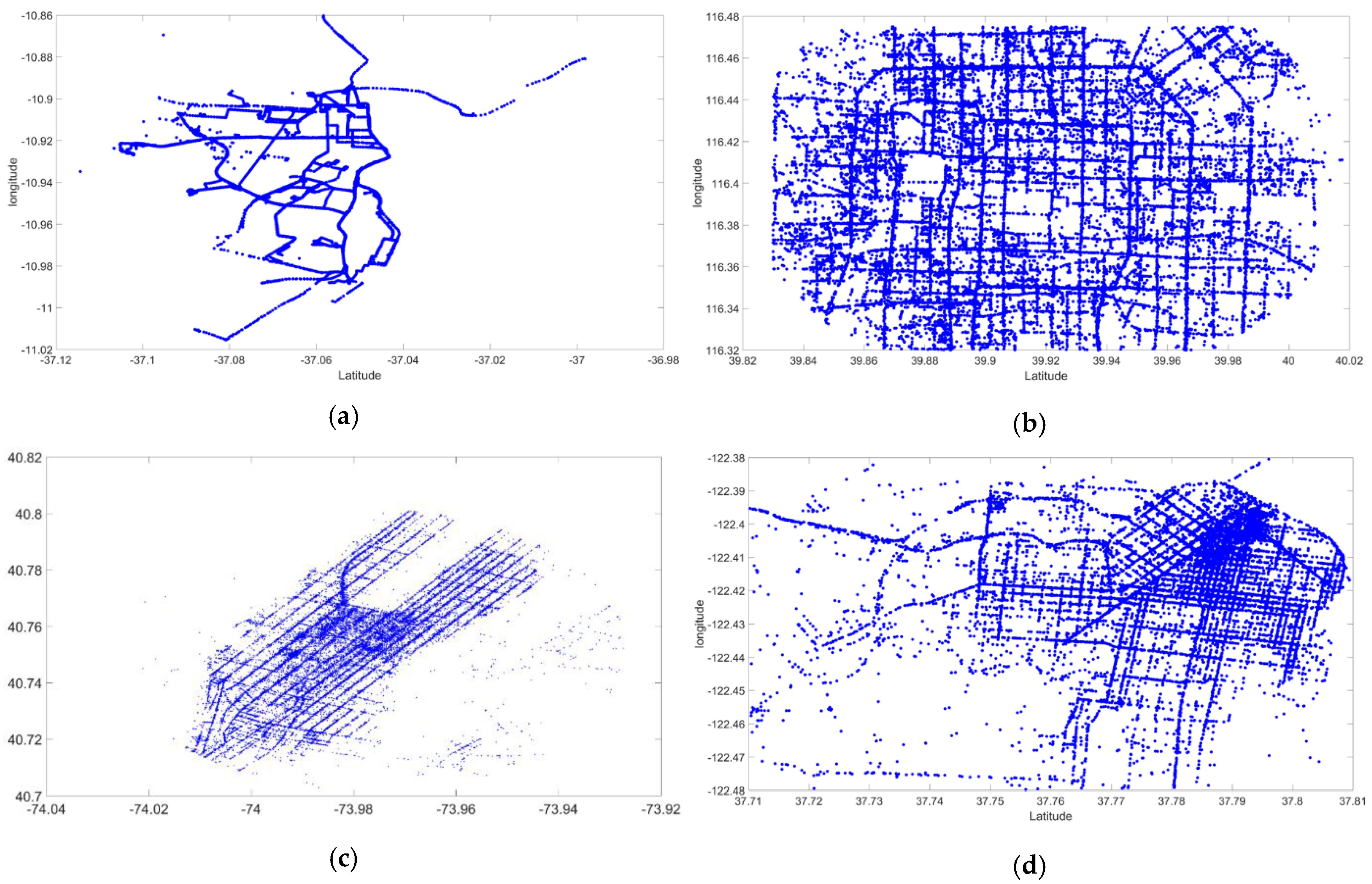
3.1. Description of Taxi GPS Data Sets on Experiments

In general, a trajectory consists of many GPS (Global Positioning System) location points, and GPS data based on trajectory data not only contains location information (longitude and latitude), but also collects time and status (e.g., speed, orientation, and status) [43,44]. These trajectory patterns of location can be usually described by OD (Origins and Destinations) [45,46,47], where OD is a common description pattern of trajectory, which can be used to describe the urban states and express city hots [45]. In this paper, the GPS data are gathered from taxi GPS points in Aracaju (Brazil) [48,49], Beijing (China) [50,51], New York (USA) [47], and San Francisco (USA) [52] (Figure 2a–d), which are often used for testing clustering algorithms. Therefore, to analyze and compare the SeedClust, GAK, GA-clustering [18], K-means, and GenClust algorithms and to achieve OD clustering, the four GPS data sets are collected and divided into OD and are then used to encode the chromosomes of genetic operation.
In Figure 1, the OD of the taxi GPS data sets are described, as follows.
(a)
The data set came from the UCI Machine Learning Repository [48,49], which is a collection of databases.
(b)
According to [50,51], this GPS trajectory data set was collected in the (Microsoft Research Asia) Geolife project by 182 users during a period of over three years (from April 2007 to August 2012). However, we only extracted the taxi GPS data points of two minutes (9:00–9:02, 2008.02.02) from Beijing, China.
(c)
According to [47], in New York City, 13,000 taxis carry over one million passengers and make 500,000 trips, totaling over 170 million trips a year. However, we extracted the taxi GPS data sets of the two minutes from New York, USA.
(d)
In [52]: This data set contained mobility traces of taxi cabs in San Francisco, USA. It contained the GPS coordinates of approximately 500 taxis collected over 2 min in the San Francisco Bay Area.
Figure 2 expresses the distributions of the taxis’ OD in a road network of the given land areas for each city (Aracaju (Brazil), Beijing (China), New York (USA), San Francisco (USA)), and the overall distributions of OD reflect the urban traffic demand change of citizens and population migration who use taxis as a transportation tool. As a result, the best hot points (seeds) will be captured and can be used to dispatch taxis and to find passengers for taxi drivers. Furthermore, traffic information and the population migration distribution will be also obtained in order to explain each city’s situation.

3.2. Clustering Results Evaluation Criteria

Validation or evaluation of the resulting clustering allowed us to analyze the result in terms of objective measures [32,53]. Depending on the information available, the clustering results can be evaluated in terms of the Silhouette coefficient (SC) [19,54], PBM [31], and DBI [19].
This type of evaluation tries to determine the quality of an obtained partition of the data without any available external information, as the data sets are real-world data. Therefore, three of the most useful evaluation criteria are employed as follows.
SC: The value of the SC index varies from −1 to 1, and a higher value indicates a better clustering result.
PBM [31]: A large value of the PBM index implies a better solution.
DBI [19]: A smaller value indicates a better clustering result, due to the distance of interior of a cluster is small, and the distance of the exterior of a cluster is greater.

3.3. Parameter Setting of Experiments for Comparison Algorithms

In the experiments on GA-clustering, K-means, GAK, GenClust, and SeedClust performed K-means clustering operation and we considered the size NIND of population equal to 30 and the termination condition is x = 120 . We maintained this consistency for all of these techniques in order to ensure a fair comparison between them. In addition, we set the number of iterations for GA-clustering, GAK, GenClust, and SeedClust to be 120 before the K-means clustering operation, with the aim to capture the best chromosome as the number of clusters and initial seeds of K-means clustering.
In the experiments, the cluster numbers in GA-clustering, K-means, GAK are user defined, and the crossover and mutation probabilities for GA-clustering and GAK are also set for P c = 0.8 and P m = 0.1 , according to the work in [18], respectively. The parameters settings of GenClust are consulted in [10]. Meanwhile, to test the impact of the number of clusters for the quality of K-means clustering results, the cluster numbers in GA-clustering, GAK, and K-means are user defined as 100, 120, 180, 174, and 140 in terms of the different taxi GPS data sets and the number of clusters of SeedClust in the same test requirement, and the number of clusters needed to be control between 2 and n . Note that the number of clusters of the SeedClust is captured automatically. Furthermore, we used GA-clustering and GAK to find the best chromosome for K-means clustering, the initial seeds of K-means are randomly generated. In this paper, the number of clusters of GenClust and SeedClust are automatically determined in terms of the initial population technique, and SeedClust also avoided being sensitive to the initial seeds in the initial population; GAK and GA-clustering used the crossover and mutation operations of the standard GA and the randomly selected the initial seeds.

3.4. Experiment Results

The experiments are implemented on four real-world taxi GPS data sets, which can be often used for testing clustering results. For each taxi GPS data set, we ran SeedClust 20 times, since it could produce different clustering results in different runs. The GA-clustering, GAK, K-means, and GenClust are also run 20 times and the clustering results are presented in Table 2, Table 3, Table 4 and Table 5. For the purpose of comparison, SC, SSE, DBI, and PBM are used to evaluate the performance of the clustering results of the taxi GPS data sets (Table 2, Table 3, Table 4 and Table 5, respectively), the tables present the maximum, minimum, average value of the clustering results for each evaluation criteria, and to verify the whole performance of SeedClust, GenClust, GAK, GA-clustering, and K-means are compared to SeedClust in the experiment. We experimentally evaluated the performance of SeedClust by comparing it with GA-clustering, GAK, K-means, and GenClust on four real-world taxi GPS data sets where each algorithm is run 20 times on each data set. In addition, the GA-clustering, GAK, GenClust, and SeedClust algorithms are based on GA, as it finds the best chromosome and then performs it to achieve the K-means clustering operation.
In particular, to analyze and compare the effectiveness and the performance of the initial population of SeedClust, two other initial population methods are used for the experiments: the initial population method of GenClust, and the density-based and K-means++ (distance-based) initialization population method (named as SeedClust (Distance), its chromosome representation and operations are the same as SeedClust, and K-means++ [14,15,55] is used for the initial seeds). In our experiment, so far, we used the improved K-means++ (density-based) for the seed selection of the initial population, and we could see that SeedClust clearly outperformed the other two existing techniques that were used in this study, as shown in Figure 2.
In Figure 3, the SSE is used to compare the performance of these initialization population methods on 20 independent trials, and SeedClust (Density) stands for SeedClust in this paper. It indicates that SeedClust with the improved K-means++ for the initial population achieved better initialization population results than SeedClust (Distance) with K-means++, and GenClust with the genes of the chromosome. Hence, we are confident that SeedClust with the improved K-means++ will win against existing initialization population techniques even more strongly and steadily. Meanwhile, the results indicate that K-means++ can be used to capture the initial seeds effectively; and, the fitness values of SeedClust are better than the other two algorithms, the curves of SeedClust are also smoother than the other two. For example, in New York, USA, the difference values of the fitness function between SeedClust and GenClust had a larger range change.
Table 2 shows the results obtained in this instance by different algorithms (GA-clustering, GAK, K-means, GenClust, and SeedClust). It shows that the results of the presented SeedClust with SC as the evaluation criterion. Note that the results are given in terms of the K-means clustering results using the best chromosome, except the K-means algorithm, and the best clustering results of the four real-world taxi GPS data sets are obtained by SeedClust. Note also that the SeedClust solutions improved the results of the GA-clustering, GAK, K-means, and GenClust algorithms. Meanwhile, we also obtained other clustering result information, as follows from Table 2. (1) The determination of the number of clusters is important in the clustering processing, for instance, when the number of clusters K are different, SC values had a significant change in the GA-clustering, GAK, and K-means algorithms; furthermore, they had the larger number of clusters, and the better of the SC values. (2) All of the SC values of SeedClust are better than GA-clustering, GAK, K-means, and seven SC values of SeedClust are better than GenClust in all of the SC values (12 values), except the same value; therefore, this indicates that the overall performance of SeedClust is better than GenClust in the SC evaluation.
Table 3 shows the results that were obtained by the different compared algorithms. The best result is obtained by the SeedClust algorithm in all of the taxi GPS data sets, and the SeedClust algorithm obtained a really good clustering result. Furthermore, the averaged SSE values indicated that SeedClust obtained a low error rate in all taxi GPS data. Meanwhile, we clearly found from Table 3 (including Table 2, Table 3, Table 4 and Table 5), the number of clusters directly impacted the clustering quality; namely, cluster numbers K are larger, so SSE values are better, and the error rates are also lower. For instance, in San Francisco, USA, the change in the SSE values are pronounced in GA-clustering, K-means, and GAK algorithms, their difference values of K = 100 and K = 140 are close to 10 or are more than 10. In particular, a larger number of clusters did not mean that the cluster quality is better; for instance, the cluster numbers between SeedClust and GenClust are equal in Aracaju, Brazil, but the SSE values of SeedClust are better than GenClust. Therefore, to obtain better clustering quality, it is difficult to guess the user number of clusters in a given data set, and the clustering results are related to different algorithm performance.
Table 4 shows the results obtained by the different compared algorithms in this paper. The best result is obtained by the SeedClust algorithm in all of the taxi GPS data sets, and the SeedClust algorithm obtained a really good clustering result; furthermore, the clustering quality is also better. DBI can be used to evaluate similar records in one cluster and dissimilar records in different clusters, and therefore Table 4 indicates that the clustering results of SeedClust are very good, did not get stuck at local minima resulting in poor clustering results, and due to the best chromosome that was used to perform the K-means clustering operation, it is also not sensitive to the quality of the initial seeds. In fact, GenClust also has these same characteristics. However, Table 4 shows that the DBI values of GenClust are a little worse than SeedClust, but its values are better than GA-clustering, GAK, and K-means.
Table 5 summarizes the clustering results that were obtained by the different algorithms considered. SeedClust with a PBM index obtained a better clustering result when the number of clusters (K) of other comparison algorithms are equal to 180, 174, and 140 (except in the San Francisco, USA data set where it not only obtained a better value, but at the beginning (before the fourth generation), its convergence speed is faster than the other comparison clustering algorithms, as shown in Figure 2d, in other words, in the San Francisco, USA data set, GenClust obtained a better clustering performance than SeedClust. However, in Aracaju, Brazil, the best measure performance is obtained by SeedClust. The values indicate the whole superiority of SeedClust, which produced a better value than those of the other GA-based clustering algorithms (GA-clustering, GAK, and GenClust) and K-means.
From the experiments, the SC, SSE, DBI, and PBM index values that were obtained by the five algorithms are presented in Table 2, Table 3, Table 4 and Table 5. The values indicate the superiority of the SeedClust algorithm, which generated better clustering result values than those of the other algorithms.
As seen from Table 6, the SeedClust clustering algorithm converged with a shorter computation time than GenClust. In other words, the convergence of the SeedClust algorithm is very good and fast without showing any fluctuation and began to converge between 5 and 15 iterations.
In Table 6, we present the results of the average execution time (20 runs per each taxi GPS data set) that is required by the five clustering algorithms. SeedClust is computationally more expensive than the existing GAK, GA-clustering, and K-means algorithm, but the differences between their complexities are not so obvious. Genetic algorithms are generally more time expensive than other basic clustering algorithms (e.g., K-means) [10]. SeedClust also uses computationally expensive operations, such as the initial population and gene rearrangement. On one hand, compared to SeedClust with GAK, GA-clustering, the operations of GAK and GA-clustering take ordinary steps without running the initial population and gene rearrangement, can only handle two equal length chromosomes and then the average execution time of GAK and GA-clustering is shorter than SeedClust and GenClust. On the other hand, when comparing SeedClust with GenClust, the computationally expensive operations of GenClust mainly focused on the initial population technique, gene rearrangement, and twin removal of each iteration, which resulted in the average execution time of GenClust being the most expensive, and the average execution time of the initial population of SeedClust ( O ( n ) ) being shorter than GenClust ( O ( n 2 ) ). Meanwhile, SeedClust reduced the complexity without performing the twin removal operation of GenClust, and in the gene rearrangement, it did not compute distances between each taxi GPS data point. Therefore, the average execution time of SeedClust is of a better level. From Table 6, we also found that the number of clusters is greater, and the execution time more expensive. In fact, the execution time of K-means is very inexpensive.

4. Conclusions

In this paper, to improve and enhance the performance of K-means clustering, SeedClust is developed for automatic K-means clustering using the best chromosome. In the SeedClust algorithm, an efficient initial population technique is improved and presented, which is used to capture the best chromosome as initial seeds and the cluster numbers of K-means clustering, therefore it can achieve better clustering quality without requiring a user to input the number of clusters. Furthermore, SeedClust could also avoid getting stuck in a local optimum since adaptive probabilities of crossover and mutation are presented and an improved gene rearrangement are used. The presented processes in the SeedClust allowed the SeedClust clustering to explore the search space more effectively without needing too high a time complexity. The SeedClust is scalable to taxi GPS data sets since the running time complexity is linear. Moreover, the superiority of the SeedClust algorithm over GA-clustering, GAK, GenClust, and K-means algorithm is demonstrated by the experiments. In particular, four real-world taxi GPS data sets are applied in these clustering algorithms, which indicated that SeedClust has effectiveness and superiority.
In future works, we will investigate an approach of density estimation, which can produce chromosomes automatically according to the distribution of GPS data points, and other intelligent algorithms such as particle swarm algorithm and ant colony algorithm will also be studied and applied in clustering operation. Meanwhile, for large and high dimensional GPS data, MapReduce-based with the GA will be studied. In addition, we will improve the experimental results by justifying the objectives of the classification of real-world GPS data.

Acknowledgments

This paper was supported by the Research and Innovation Team of Universities and Colleges in Sichuan Province of China (15DT0039, 16DT0033), the Sichuan tourism youth expert training program (SCTYETP2017L02), and the Sichuan Science and Technology Program (18ZDYF3245, 2016GZ0140).

Author Contributions

All authors contributed to this paper. Xianbing Zhou, Hongjiang Ma, and Fang Miao conceived the original idea for the study; Xianbing Zhou wrote the paper, Xiangbing Zhou, Hongjiang Ma performed the experiments; and Xianbing Zhou analyzed the experiment results and revised the manuscript. All authors read and approved the submitted manuscript.

Conflicts of Interest

The authors declare no conflict of interest.

References

  1. Han, J.; Pei, J.; Kamber, M. Data Mining: Concepts and Techniques; Elsevier: New York, NY, USA, 2011. [Google Scholar]
  2. Jain, A.K. Data clustering: 50 years beyond k-means. Pattern Recog. Lett. 2010, 31, 651–666. [Google Scholar] [CrossRef]
  3. Kumar, K.M.; Reddy, A.R.M. An efficient k-means clustering filtering algorithm using density based initial cluster centers. Inf. Sci. 2017, 418, 286–301. [Google Scholar] [CrossRef]
  4. Bai, L.; Cheng, X.; Liang, J.; Shen, H.; Guo, Y. Fast density clustering strategies based on the k-means algorithm. Pattern Recognit. 2017, 71, 375–386. [Google Scholar] [CrossRef]
  5. Taherdangkoo, M.; Bagheri, M.H. A powerful hybrid clustering method based on modified stem cells and fuzzy c-means algorithms. Eng. Appl. Artif. Intell. 2013, 26, 1493–1502. [Google Scholar] [CrossRef]
  6. Wishart, D. K-Means Clustering with Outlier Detection, Mixed Variables and Missing Values; Springer: Berlin/Heidelberg, Germany, 2003; pp. 216–226. [Google Scholar]
  7. Jianjun, C.; Xiaoyun, C.; Haijuan, Y.; Mingwei, L. An enhanced k-means algorithm using agglomerative hierarchical clustering strategy. In Proceedings of the International Conference on Automatic Control and Artificial Intelligence (ACAI 2012), Xiamen, China, 3–5 March 2012; pp. 407–410. [Google Scholar]
  8. Akodjènou-Jeannin, M.-I.; Salamatian, K.; Gallinari, P. Flexible grid-based clustering. In Proceedings of the 11th European Conference on Principles of Data Mining and Knowledge Discovery, Warsaw, Poland, 17–21 September 2007; pp. 350–357. [Google Scholar]
  9. Zhao, Q.; Shi, Y.; Liu, Q.; Fränti, P. A grid-growing clustering algorithm for geo-spatial data. Pattern Recognit. Lett. 2015, 53, 77–84. [Google Scholar] [CrossRef]
  10. Rahman, M.A.; Islam, M.Z. A hybrid clustering technique combining a novel genetic algorithm with k-means. Knowl. Based. Syst. 2014, 71, 345–365. [Google Scholar] [CrossRef]
  11. Celebi, M.E.; Kingravi, H.A.; Vela, P.A. A comparative study of efficient initialization methods for the k-means clustering algorithm. Expert Syst. Appl. 2013, 40, 200–210. [Google Scholar] [CrossRef]
  12. Rahman, A.; Islam, Z. Seed-detective: A novel clustering technique using high quality seed for k-means on categorical and numerical attributes. In Proceedings of the Ninth Australasian Data Mining Conference, Ballarat, Australia, 1–2 December 2011; Australian Computer Society Inc.: Sydney, Australia, 2011; Volume 121, pp. 211–220. [Google Scholar]
  13. Rahman, M.A.; Islam, M.Z. Crudaw: A novel fuzzy technique for clustering records following user defined attribute weights. In Proceedings of the Tenth Australasian Data Mining Conference, Sydney, Australia, 5–7 December 2012; Australian Computer Society Inc.: Sydney, Australia, 2012; Volume 134, pp. 27–41. [Google Scholar]
  14. Arthur, D.; Vassilvitskii, S. K-means++: The advantages of careful seeding. In Proceedings of the Eighteenth Annual ACM-SIAM Symposium on Discrete Algorithms, New Orleans, LA, USA, 7–9 January 2007; Society for Industrial and Applied Mathematics: Philadelphia, PA, USA, 2007; pp. 1027–1035. [Google Scholar]
  15. Beg, A.; Islam, M.Z.; Estivill-Castro, V. Genetic algorithm with healthy population and multiple streams sharing information for clustering. Knowl. Based Syst. 2016, 114, 61–78. [Google Scholar] [CrossRef]
  16. Bandyopadhyay, S.; Maulik, U. An evolutionary technique based on k-means algorithm for optimal clustering in RN. Inf. Sci. 2002, 146, 221–237. [Google Scholar] [CrossRef]
  17. Maulik, U.; Bandyopadhyay, S. Genetic algorithm-based clustering technique. Pattern Recognit. 2000, 33, 1455–1465. [Google Scholar] [CrossRef]
  18. Chang, D.-X.; Zhang, X.-D.; Zheng, C.-W. A genetic algorithm with gene rearrangement for k-means clustering. Pattern Recognit. 2009, 42, 1210–1222. [Google Scholar] [CrossRef]
  19. Agustı, L.; Salcedo-Sanz, S.; Jiménez-Fernández, S.; Carro-Calvo, L.; Del Ser, J.; Portilla-Figueras, J.A. A new grouping genetic algorithm for clustering problems. Expert Syst. Appl. 2012, 39, 9695–9703. [Google Scholar] [CrossRef]
  20. Liu, Y.; Wu, X.; Shen, Y. Automatic clustering using genetic algorithms. Appl. Math. Comput. 2011, 218, 1267–1279. [Google Scholar] [CrossRef]
  21. Hruschka, E.R.; Campello, R.J.; Freitas, A.A. A survey of evolutionary algorithms for clustering. IEEE Trans. Syst. Man Cybern. Part C (Appl. Rev.) 2009, 39, 133–155. [Google Scholar] [CrossRef]
  22. He, H.; Tan, Y. A two-stage genetic algorithm for automatic clustering. Neurocomputing 2012, 81, 49–59. [Google Scholar] [CrossRef]
  23. Wei, L.; Zhao, M. A niche hybrid genetic algorithm for global optimization of continuous multimodal functions. Appl. Math. Comput. 2005, 160, 649–661. [Google Scholar] [CrossRef]
  24. Martín, D.; Alcalá-Fdez, J.; Rosete, A.; Herrera, F. Nicgar: A niching genetic algorithm to mine a diverse set of interesting quantitative association rules. Inf. Sci. 2016, 355, 208–228. [Google Scholar] [CrossRef]
  25. Deng, W.; Zhao, H.; Zou, L.; Li, G.; Yang, X.; Wu, D. A novel collaborative optimization algorithm in solving complex optimization problems. Soft Comput. 2017, 21, 4387–4398. [Google Scholar] [CrossRef]
  26. Pirim, H.; Ekşioğlu, B.; Perkins, A.; Yüceer, Ç. Clustering of high throughput gene expression data. Comput. Oper. Res. 2012, 39, 3046–3061. [Google Scholar] [CrossRef] [PubMed]
  27. Chowdhury, A.; Das, S. Automatic shape independent clustering inspired by ant dynamics. Swarm Evolut. Comput. 2012, 3, 33–45. [Google Scholar] [CrossRef]
  28. Krishna, K.; Murty, M.N. Genetic k-means algorithm. IEEE Trans. Syst. Man Cybern. Part B (Cyber.) 1999, 29, 433–439. [Google Scholar] [CrossRef] [PubMed]
  29. GitHub. Real-World Taxi-GPS Data Sets. Available online: https://github.com/bigdata002/Location-data-sets (accessed on 20 April 2018).
  30. Davies, D.L.; Bouldin, D.W. A cluster separation measure. IEEE Trans. Pattern Anal. 1979, PAMI-1, 224–227. [Google Scholar] [CrossRef]
  31. Pakhira, M.K.; Bandyopadhyay, S.; Maulik, U. Validity index for crisp and fuzzy clusters. Pattern Recognit. 2004, 37, 487–501. [Google Scholar] [CrossRef]
  32. Zhou, X.; Gu, J.; Shen, S.; Ma, H.; Miao, F.; Zhang, H.; Gong, H. An automatic k-means clustering algorithm of GPS data combining a novel niche genetic algorithm with noise and density. ISPRS Int. J. Geo-Inf. 2017, 6, 392. [Google Scholar] [CrossRef]
  33. Lotufo, R.A.; Zampirolli, F.A. Fast multidimensional parallel Euclidean distance transform based on mathematical morphology. In Proceedings of the XIV Brazilian Symposium on Computer Graphics and Image Processing, Florianopolis, Brazil, 15–18 October 2001; pp. 100–105. [Google Scholar]
  34. Juan, A.; Vidal, E. In Comparison of four initialization techniques for the k-medians clustering algorithm. In Proceedings of the Joint IAPR International Workshops on Statistical Techniques in Pattern Recognition (SPR) and Structural and Syntactic Pattern Recognition (SSPR), Alicante, Spain, 30 August–1 September 2000; pp. 842–852. [Google Scholar]
  35. Celebi, M.E. Improving the performance of k-means for color quantization. Image Vis. Comput. 2011, 29, 260–271. [Google Scholar] [CrossRef]
  36. Spaeth, H. Cluster Dissection and Analysis, Theory, FORTRAN Programs, Examples; Ellis Horwood: New York, NY, USA, 1985. [Google Scholar]
  37. Cao, F.; Liang, J.; Bai, L. A new initialization method for categorical data clustering. Expert Syst. Appl. 2009, 36, 10223–10228. [Google Scholar] [CrossRef]
  38. Silverman, B.W. Density Estimation for Statistics and Data Analysis; CRC Press: Boca Raton, FL, USA, 1986; Volume 26. [Google Scholar]
  39. Patwary, M.M.A.; Palsetia, D.; Agrawal, A.; Liao, W.-K.; Manne, F.; Choudhary, A. Scalable parallel optics data clustering using graph algorithmic techniques. In Proceedings of the 2013 International Conference for High Performance Computing, Networking, Storage and Analysis (SC), Denver, CO, USA, 17–22 November 2013; pp. 1–12. [Google Scholar]
  40. Bai, L.; Liang, J.; Dang, C. An initialization method to simultaneously find initial cluster centers and the number of clusters for clustering categorical data. Knowl. Based Syst. 2011, 24, 785–795. [Google Scholar] [CrossRef]
  41. Bahmani, B.; Moseley, B.; Vattani, A.; Kumar, R.; Vassilvitskii, S. Scalable k-means++. Proc. VLDB Endow. 2012, 5, 622–633. [Google Scholar] [CrossRef]
  42. Xiao, J.; Yan, Y.P.; Zhang, J.; Tang, Y. A quantum-inspired genetic algorithm for k-means clustering. Expert Syst. Appl. 2010, 37, 4966–4973. [Google Scholar] [CrossRef]
  43. Tang, J.; Liu, F.; Wang, Y.; Wang, H. Uncovering urban human mobility from large scale taxi GPS data. Phys. A Stat. Mech. Appl. 2015, 438, 140–153. [Google Scholar] [CrossRef]
  44. Ekpenyong, F.; Palmer-Brown, D.; Brimicombe, A. Extracting road information from recorded GPS data using snap-drift neural network. Neurocomputing 2009, 73, 24–36. [Google Scholar] [CrossRef]
  45. Lu, M.; Liang, J.; Wang, Z.; Yuan, X. Exploring OD patterns of interested region based on taxi trajectories. J. Vis. 2016, 19, 811–821. [Google Scholar] [CrossRef]
  46. Moreira-Matias, L.; Gama, J.; Ferreira, M.; Mendes-Moreira, J.; Damas, L. Time-evolving OD matrix estimation using high-speed GPS data streams. Expert Syst. Appl. 2016, 44, 275–288. [Google Scholar] [CrossRef]
  47. Ferreira, N.; Poco, J.; Vo, H.T.; Freire, J.; Silva, C.T. Visual exploration of big spatio-temporal urban data: A study of new york city taxi trips. IEEE Trans. Vis. Comput. Graph. 2013, 19, 2149–2158. [Google Scholar] [CrossRef] [PubMed]
  48. Cruz, M.O.; Macedo, H.; Guimaraes, A. Grouping similar trajectories for carpooling purposes. In Proceedings of the 2015 Brazilian Conference on Intelligent Systems (BRACIS), Natal, Brazil, 4–7 November 2015; pp. 234–239. [Google Scholar]
  49. Dua, D.; Karra, T.E. Machine Learning Repository (UCI). 731. Available online: https://archive.ics.uci.edu/ml/datasets.html (accessed on 20 April 2018).
  50. Zheng, Y.; Liu, Y.; Yuan, J.; Xie, X. Urban computing with taxicabs. In Proceedings of the 13th International Conference on Ubiquitous Computing, Beijing, China, 17–21 September 2011; pp. 89–98. [Google Scholar]
  51. Yuan, J.; Zheng, Y.; Xie, X.; Sun, G. Driving with knowledge from the physical world. In Proceedings of the ACM SIGKDD International Conference on Knowledge Discovery and Data Mining, San Diego, CA, USA, 21–24 August 2011; pp. 316–324. [Google Scholar]
  52. Piorkowski, M.; Natasa, S.D. Matthias Grossglauser. Crawdad Dataset Epfl/Mobility (v. 2009-02-24). 2009. Available online: http://crawdad.org/epfl/mobility/20090224 (accessed on 20 April 2018).
  53. Halkidi, M.; Batistakis, Y.; Vazirgiannis, M. On clustering validation techniques. J. Intell. Inf. Syst. 2001, 17, 107–145. [Google Scholar] [CrossRef]
  54. Rousseeuw, P.J. Silhouettes: A graphical aid to the interpretation and validation of cluster analysis. J. Comput. Appl. Math. 1987, 20, 53–65. [Google Scholar] [CrossRef]
  55. Islam, M.Z.; Estivill-Castro, V.; Rahman, M.A.; Bossomaier, T. Combining k-means and a genetic algorithm through a novel arrangement of genetic operators for high quality clustering. Expert Syst. Appl. 2018, 91, 402–417. [Google Scholar] [CrossRef]
Figure 1. Diagram of SeedClust using the density-based and improved K-means++.
Information 09 00101 g001
Figure 2. Distribution of Origins and Destinations (OD) of taxi GPS data: (a) Aracaju (Brazil); (b) Beijing (China); (c) New York (USA); and (d) San Francisco (USA).
Information 09 00101 g002
Figure 3. The fitness values of the initial population for the four real-world taxi GPS data sets are obtained by SeedClust (Density), SeedClust (Distance) and GenClust over 20 independence experiments: (a) Aracaju (Brazil); (b) Beijing (China); (c) New York (USA); and (d) San Francisco (USA).
Information 09 00101 g003
Table 1. The experimental data sets of taxi Global Positioning System (GPS) data.
Taxi GPS Data SetLand AreaThe Number of GPS Taxi Data PointsThe Number of Clusters
GA-Clustering, GAK, K-meansGenClustNoiseClust
Aracaju (Brazil)0.14 × 0.1616,513100, 120128128
Beijing (China)1.20 × 0.1635,541100, 180188188
New York (USA)0.12 × 0.1232,786100, 174173181
San Francisco (USA)0.10 × 0.1021,826100, 140147147
Table 2. The maximum, mean, and minimum values of Silhouette coefficient obtained by genetic algorithms (GA)-clustering, GAK, K-means, and SeedClust algorithms for 20 different runs for four real-world taxi GPS data sets.
Aracaju (Brazil)GA-ClusteringK-MeansGAKGenClustSeedClust
K = 100K = 120K = 100K = 120K = 100K = 120K = 128K = 128
Max0.94370.95070.95210.95860.95310.95900.96660.9628
Mean0.94040.94710.94920.95600.95120.95770.95810.9608
Min0.93370.94520.94370.95380.94910.95540.95000.9555
Beijing (China)GA-ClusteringK-MeansGAKGenClustSeedClust
K = 100K = 180K = 100K = 180K = 100K = 180K = 188K = 188
Max0.89350.92110.90440.93180.90470.93220.93390.9342
Mean0.89100.91990.90310.93060.90360.93120.93320.9332
Min0.88800.91880.90190.92910.90240.93040.92680.9306
New York (USA)GA-ClusteringK-MeansGAKGenClustSeedClust
K = 100K = 174K = 100K = 174K = 100K = 174K = 173K = 181
Max0.90350.92790.91390.93670.91360.93660.93590.9382
Mean0.90120.92550.91210.93580.91250.93580.93370.9370
Min0.89900.92260.91080.93430.91100.93510.93230.9322
San Francisco (USA)GA-ClusteringK-MeansGAKGenClustSeedClust
K = 100K = 140K = 100K = 140K = 100K = 140K = 147K = 147
Max0.91210.92410.92110.93450.92240.93520.94240.9373
Mean0.90890.92230.91920.93170.92070.93400.93480.9349
Min0.90620.91990.91510.92960.91800.93190.92420.9309
The bold font indicates the best value for each taxi GPS data set.
Table 3. The maximum, mean, and minimum values of SSE obtained by GA-clustering, GAK, K-means, and SeedClust algorithms for 20 different runs for four real-world taxi GPS data sets.
Aracaju (Brazil)GA-ClusteringK-MeansGAKGenClustSeedClust
K = 100K = 120K = 100K = 120K = 100K = 120K = 128K = 128
Max56.800628.624426.446721.441623.693520.652720.280219.8027
Mean30.920627.628423.468520.333522.405419.281719.470617.7361
Min28.496925.611022.330019.221821.434418.561718.542516.8413
Beijing (China)GA-ClusteringK-MeansGAKGenClustSeedClust
K = 100K = 180K = 100K = 180K = 100K = 180K = 188K = 188
Max243.2074177.8441192.6010139.9668190.9683135.9318131.4806134.4856
Mean233.2443174.7318189.4489135.8667188.5583134.3636130.3514129.5278
Min225.5980170.0283186.4393133.2682187.0371132.8659128.9393127.2393
New York (USA)GA-ClusteringK-MeansGAKGenClustSeedClust
K = 100K = 174K = 100K = 174K = 100K = 174K = 173K = 181
Max78.032861.334464.463848.003764.414746.972447.516349.0167
Mean75.874659.416663.690546.753563.192946.525046.698145.0523
Min56.800657.748162.690746.047662.405046.085145.514144.6943
San Francisco (USA)GA-ClusteringK-MeansGAKGenClustSeedClust
K = 100K = 140K = 100K = 140K = 100K = 140K = 147K = 147
Max56.800647.804645.210738.178043.736936.286236.048735.8719
Mean54.056446.261243.381036.947242.297835.387634.592934.3558
Min51.825744.927742.125135.675941.346734.210633.730933.3992
The bold font indicates the best value for each taxi GPS data set.
Table 4. The maximum, mean, and minimum values of Davies-Bouldin index (DBI) obtained by GA-clustering, GAK, K-means, and SeedClust algorithms for 20 different runs for four real-world taxi GPS data sets.
Aracaju (Brazil)GA-ClusteringK-MeansGAKGenClustSeedClust
K = 100K = 120K = 100K = 120K = 100K = 120K = 128K = 128
Max13.923133.65730.67540.69040.66130.64380.64490.6488
Mean6.19808.23780.63460.63220.62810.62060.63280.6003
Min2.21462.14670.62000.59110.59170.59120.61270.5689
Beijing (China)GA-ClusteringK-MeansGAKGenClustSeedClust
K = 100K = 180K = 100K = 180K = 100K = 180K = 188K = 188
Max2.62584.49560.82420.80140.81900.79810.80970.7916
Mean1.79452.53570.80060.78440.79890.78450.79570.7747
Min1.39161.66380.77930.76850.78040.77240.78210.7582
New York (USA)GA-ClusteringK-MeansGAKGenClustSeedClust
K = 100K = 174K = 100K = 174K = 100K = 174K = 173K = 181
Max3.09593.76810.82560.80330.84850.80910.80550.8090
Mean1.95522.26820.80430.78680.80520.79130.79440.7881
Min1.51011.58620.78520.77310.78520.77880.78160.7691
San Francisco (USA)GA-ClusteringK-MeansGAKGenClustSeedClust
K = 100K = 140K = 100K = 140K = 100K = 140K = 147K = 147
Max5.34886.03870.81030.81190.82240.80650.80840.8013
Mean2.55213.02170.79400.79150.79880.78770.78450.7794
Min1.76592.09310.76810.77230.78160.77530.76760.7598
The bold font indicates the best value for each taxi GPS data set.
Table 5. The maximum, mean, and minimum values of PBM obtained by GA-clustering, GAK, K-means, and SeedClust algorithms for 20 different runs for four real-world taxi GPS data sets.
Aracaju (Brazil)GA-ClusteringK-MeansGAKGenClustSeedClust
K = 100K = 120K = 100K = 120K = 100K = 120K = 128K = 128
Max0.02480.02280.03110.03010.03240.03190.03080.0328
Mean0.02180.02090.02960.02840.03100.03020.02980.0312
Min0.01970.01900.01970.02670.02920.02800.02880.0300
Beijing (China)GA-ClusteringK-MeansGAKGenClustSeedClust
K = 100K = 180K = 100K = 180K = 100K = 180K = 188K = 188
Max0.01670.01250.01950.01560.01940.01550.01510.0156
Mean0.01560.01190.01910.01510.01910.01530.01500.0153
Min0.01470.01160.01870.01470.01870.01490.01480.0149
New York (USA)GA-ClusteringK-MeansGAKGenClustSeedClust
K = 100K = 174K = 100K = 174K = 100K = 174K = 173K = 181
Max0.00910.00680.01060.00830.01050.00850.00830.0086
Mean0.00840.00640.01010.00820.01020.00830.00820.0083
Min0.00770.00600.00980.00790.00990.00810.00810.0079
San Francisco (USA)GA-ClusteringK-MeansGAKGenClustSeedClust
K = 100K = 140K = 100K = 140K = 100K = 140K = 147K = 147
Max0.01130.00960.01280.01130.01370.01170.01230.0125
Mean0.01000.00870.01240.01100.01280.01110.01160.0114
Min0.00880.00750.01180.01010.01230.01050.01090.0105
The bold font indicates the best value for each taxi GPS data set; the oblique bold indicates the best change value when the number of clusters (K) are increased from 100 to 120, 180, 174, and 140 for each taxi GPS data set.
Table 6. The average computational times (in minutes) of the clustering algorithms for four taxi GPS data sets.
Taxi GPS Data SetGA-ClusteringK-MeansGAKGenClustSeedClust
K = 100K = 120K = 100K = 180K = 100K = 174
Aracaju (Brazil)1.49282.00000.05100.05871.48362.071543.62783.2718
Beijing (China)3.28286.23040.11200.20113.28286.8314114.248011.9476
New York (USA)3.48866.60530.10190.17733.94297.0315129.553010.9130
San Francisco (USA)2.17343.27010.07360.09442.13913.273065.33915.3727

