Article

A Fuzzy EWMA Attribute Control Chart to Monitor Process Mean

by
Muhammad Zahir Khan
1,
Muhammad Farid Khan
1,
Muhammad Aslam
2,*,
Seyed Taghi Akhavan Niaki
3 and
Abdur Razzaque Mughal
1
1
Department of Mathematics and Statistics, Riphah International University, Islamabad 45210, Pakistan
2
Department of Statistics, Faculty of Science, King Abdulaziz University, Jeddah 21551, Saudi Arabia
3
Department of Industrial Engineering, Sharif University of Technology, P.O. Box 11155-9414 Azadi Ave., Tehran 15119-43943, Iran
*
Author to whom correspondence should be addressed.
Information 2018, 9(12), 312; https://doi.org/10.3390/info9120312
Submission received: 30 September 2018 / Revised: 18 November 2018 / Accepted: 4 December 2018 / Published: 7 December 2018

Abstract

:
Conventional control charts are one of the most important techniques in statistical process control which are used to assess the performance of processes to see whether they are in- or out-of-control. As traditional control charts deal with crisp data, they are not suitable to study unclear, vague, and fuzzy data. In many real-world applications, however, the data to be used in a control charting method are not crisp since they are approximated due to environmental uncertainties and systematic ambiguities involved in the systems under investigation. In these situations, fuzzy numbers and linguistic variables are used to grab such uncertainties. That is why the use of a fuzzy control chart, in which fuzzy data are used, is justified. As an exponentially weighted moving average (EWMA) scheme is usually used to detect small shifts, in this paper a fuzzy EWMA (F-EWMA) control chart is proposed to detect small shifts in the process mean when fuzzy data are available. The application of the newly developed fuzzy control chart is illustrated using real-life data.

1. Introduction and Literature Review

Process performance and proficiency can be enhanced by decreasing variability. This can be attained with the assistance of statistical process control (SPC) methods. The aim of a statistical process control method is to achieve stability and to improve the efficiency of a process by reducing the variability involved. Conventional control charts are one of the tools to achieve this objective. Conventional control charts, also known as Shewhart control charts, are used to detect shifts in a process. The mostly used Shewhart control charts when a variable quality characteristic is monitored include “x-bar and range” and “x-bar and s(standard deviation)” control charts. However, these charts are not able to detect small shifts. Another problem is that these charts are not independent of each other. In order to detect small shifts in the process mean or in the process variation, an exponentially weighted moving average (EWMA) scheme is used. Nonetheless, the construction method and the interpretation involved in a traditional Shewhart chart are different from the ones in an EMWA control chart. In other words, the plot of a Shewhart control chart shows independent data points and follows the law of the sampling distribution of the statistic. However, in an EWMA or in a cumulative sum (CUSUM) scheme, a statistic corresponding to a parameter is estimated directly. When a process monitored using an EWMA or a CUSUM control chart goes out-of-control, the data moves gradually to the next level. Otherwise, the chart will show a discrepancy about the centerline with small variations when the process is in-control [1]. In addition, the EWMA and the CUSUM control charts are usually used to detect small shifts in a process. Yang et al. [2] proposed a new EWMA control chart to monitor the mean of a process with a variable quality characteristic. It can be applied in a situation when the distribution of the available process data is either unidentified or non-normal. Although their chart was shown to have a very good performance, the Arcsine-EWMA control chart developed also by Yang et al. [2] performed better. To monitor processes with attribute characteristics, however, the p and the c charts are the most widely employed schemes.
A control chart consists of three lines; the center (average) line, the upper, and the lower control limits (lines). The strength of any chart can be judged by its ability to identify the shifts and the irregularity of a process. This strength is directly related to the choice of its control limits when the chart is designed. This also applies to fuzzy control charts introduced by Raz & Wang [3] for the first time, when they suggested the use of two approaches: a probabilistic approach and a membership approach. Ever since, this type of chart has gained much interest in the literature. The control charts are recommended by Kanagawa [4] for linguistic terms obtained by experts’ opinion and regarded as fuzzy data are different from the one proposed by Wang [5]. It monitors not only the process average but also the process variability. In order to decrease the emergence of false alarms, as well as to enhance the speed to identify actual errors, El-Shal [6] used fuzzy logic to amend SPC rules. Rowlands & Wang [7] proposed a fuzzy SPC evaluation and control method which combined the traditional statistical process control methodology with an intelligent system approach. Gülbay & Ruan [8] recommended α-cut control charts to monitor attribute data to adjust the stiffness of the inspection using triangular fuzzy numbers. Cheng [9] developed a fuzzy control chart to deal with a process that gives fuzzy outcomes. He designed two fuzzy control charts to directly observe the fuzzy results in order to determine the process quality. A direct fuzzy approach was introduced by Gülbay [10] as a substitute to fuzzy control charts. This approach can be applied on fuzzy attribute data obtained by vague events. To control process mean, Faraz [11] developed a fuzzy control chart with a warning line alongside an upper control limit. Erginel [12] presented the theoretical structure of fuzzy individual and moving range control charts with α-cuts using α-level fuzzy median transformation techniques. Sentürk [13] designed fuzzy ( X ¯ ˜ R   ˜ ) and ( X ˜ S ˜ ) charts with α-cuts using α-level fuzzy midrange transformation techniques. They used triangular fuzzy membership functions with fuzzy numbers (a, b, c). Later, Sentürk [14] proposed a fuzzy regression control chart. Fuzzy variable control charts deal with fuzzy variable data, for example, fuzzy measurement (length, width, height). On the other hand, fuzzy attribute control charts study qualitative data which cannot be expressed in numbers, for example, fuzzy attributes (defective, nonconformities). While some fuzzy variable control charts include ( X ¯ ˜ R   ˜ ) and ( X ˜ S ˜ ) , fuzzy attribute control charts include ( p ˜ , c ˜ , u ˜ ). If the quality-related characteristics cannot be represented in arithmetic form, such as characteristics for appearance, softness, color, and so forth, then control charts for attributes are used. Product units are either classified as conforming or nonconforming, depending upon whether or not they meet specifications, or the number of nonconformities (deviations from specifications) per unit is counted. There are four major types of control charts. The first type, the x-chart (and related x-bar, r-, and s-charts), is a generic and simple control chart. The x-chart is designed to be used primarily with variable data, which are usually measurements, such as the length of an object, processing time, or the number of objects produced per period. The other types of control charts are the p-charts, which are used with binomial data, the c-charts, which are used for Poisson processes, and the u-charts, generally designed for counting defects per sample when the sample size varies for each inspection. According to Kaya & Kahraman [15] when the value is given as “around” and ”approximate”, a triangular fuzzy number is mostly used, and when the value is given as “between”, two trapezoidal fuzzy numbers are used. The examples of a triangular fuzzy number and trapezoidal fuzzy numbers are approximate speed (20 km) and speed between (25 km to 30 km). If the vertex of a trapezoidal fuzzy number has taken a common value, it is transformed into a triangular fuzzy number.
Sentürk et al. [16] introduced fuzzy u ˜ control charts to monitor fuzzy attribute data. Kaya [15] designed fuzzy control charts for fuzzy measurements of the related quality characteristics. A fuzzy multivariate exponentially weighted moving average (F-MEWMA) control chart was suggested by Alipour [17] to be implemented on a process in the food industry. Sentürk [18] suggested a fuzzy EWMA (F-EWMA) control chart to study fuzzy univariate process data using α-cuts. The design of this scheme is based on using triangular fuzzy numbers and the fuzzy midrange technique to study fuzzy data by converting it into scalar form. Their future recommendation was to apply the same technique on conventional control charts to make them able to work in fuzzy environment. Khademi [19] developed two fuzzy approaches to design control charts observing fuzzy averages and ranges. These approaches that are based on fuzzy mode and fuzzy base rules are better in the sense they do not use a defuzzification method and are more informative than the existing fuzzy control charts. They demonstrated the performance of their charts with the help of a real-life example. Recently, Kahraman [20] introduced two fuzzy control charts to monitor fuzzy outcomes in order to see whether a process is in-control or out-of-control. It should be mentioned that the capability of a process can also be measured with the help of a fuzzy control chart to check whether a process is in- or out-of-control [15].
The recommendation provided by Sentürk [18] is utilized in the current paper on another conventional scheme proposed by Yang et al. [2] to design a new fuzzy EWMA chart that can be used to detect small shifts on the mean of a process in a fuzzy environment. This makes the newly design chart more applicable, more flexible, and more informative in real-life quality control problems. It gives practitioners an opportunity to study intermediate values of fuzzy parameters that is not possible with crisp parameters in a fuzzy environment. Although Yang et al. [2] used approximate values in their example, they are treated as fuzzy numbers in the current work, based on which a fuzzy form of his chart is proposed. This newly developed fuzzy chart will be applied on real-life data collected from the food industry.
The structure of the remainder of the paper is as follows. A brief background on the fuzzy variable and attribute control charts and the fuzzy transformation approaches is given in Section 2. The conventional EWMA chart proposed by Yang et al. [2] is described in Section 3 in detail. The fuzzy EWMA chart to monitor the process mean in a fuzzy environment is designed in Section 4. The application of the proposed chart is investigated in Section 5 using cooking oil filling data. Finally, the conclusion and recommendation for future studies are given in Section 6.

2. The Fuzzy Attribute and Variable Schemes

Fuzziness and ambiguity may have several reasons including lack of knowledge, chance, imprecision, incompetence to perform adequate measurements, and inborn fuzziness in the process. Fuzziness in humanistic systems is dealt with in a mathematical way with the help of fuzzy sets [21]. The fuzzy set theory provides an opportunity to study human subjectivity in a scientific manner with the assistance of fuzzy sets [22].

2.1. Fuzzy Transformation Approaches

When fuzzy data are used, it is essential to represent the fuzzy sets linked with the linguistic data in the sample by some scalar (transformation) numbers for additional calculations. There are four fuzzy measures of central tendencies in the literature used to calculate transformed numbers. These measures include (1) fuzzy mean, (2) fuzzy median, (3) fuzzy mode, and (4) fuzzy midrange ([3,5]).

2.2. Some Fuzzy Formulae

The formula to compute the fuzzy average is [21]:
f a v g = x = 0 1 x U F ( X ) x = 0 1 U F ( X ) .
To determine the fuzzy median, the curve under the membership function is divided into two halves. As a result, the fuzzy median becomes
f m e d i a n = a f m e d U F ( X ) d x .
The fuzzy mode is the value of the base variable where the membership function equals 1. Thus,
f m o d e = { X U F ( X ) = 1 } .
The fuzzy mid-range is the mean end points of the α-cut as
f α m r = 1 2 ( a α + a c ) .
According to [18], there are no solid reasons to decide which technique is better to use, but most researchers applied the α-level fuzzy midrange technique in their works due to its simple form of formula.

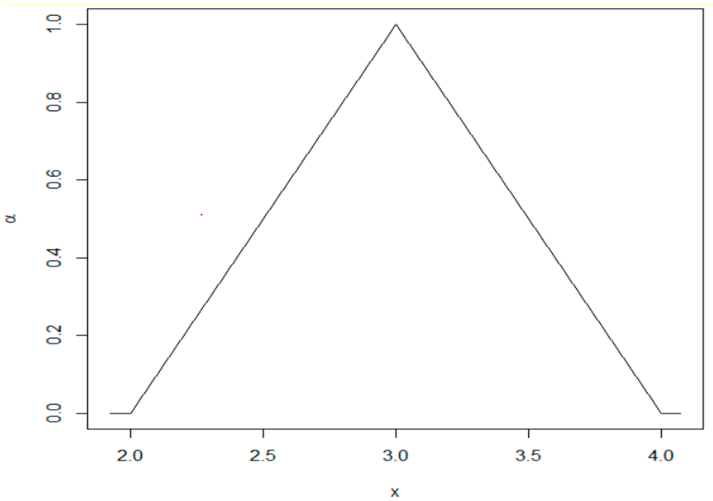
2.3. Triangular Fuzzy Number

A triangular fuzzy number A ˜ is a fuzzy number with its membership function defined by three numbers a 1 < a 2 < a 3 where the base of the triangle is the interval [ a 1 , a 3 ] and the vertex is at X = a 2 .
Example. 
In the following Figure 1, there is triangular number defined by three numbers (a1 = 2, a2 = 3, a3 = 4), where the base of the triangle is the interval [ 2 ,   4 ] and the vertex is at X = 3 .
The basic forms of the variable and the attribute fuzzy control charts were given in [20]. The attribute control charts are p ˜ -chart, n p ˜ -chart, c ˜ -chart, and u ˜ -chart, while the variable charts include ( X ¯ ˜ R ˜ ) and ( X ˜ S ˜ ) schemes. Fuzzy forms of these charts make them more flexible, sensitive, and informative. A fuzzy variable quality characteristic in m samples, each with the size of n was represented using a triangular fuzzy number denoted by X i ˜ = ( X i a , X i b , X i c ) , where i = 1 , 2 , 3 , , m . In addition, each sample in a fuzzy attribute chart, for example, the n p ˜ control chart developed to study the number of nonconforming units in a fuzzy environment, was presented by a triangular fuzzy number ( d i a , d i b , d i c ) with the mean of ( n p ¯ a , n p ¯ b , n p ¯ c ) , where n p ¯ a = i = 1 m d i a m , n p ¯ b = i = 1 m d i b m , and   n p ¯ c = i = 1 m d i c m . Hence, the control limits of the fuzzy n p ˜ chart are [20]:
U C L ˜ = ( n p ¯ a + 3 n p ¯ a ( 1 p ¯ a ) , n p ¯ b + 3 n p ¯ b ( 1 p ¯ b ) , n p ¯ c + 3 n p ¯ c ( 1 p ¯ c ) )
C L ˜ = ( n p ¯ a , n p ¯ b , n p ¯ c )
L C L ˜ = ( n p ¯ a 3 n p ¯ a ( 1 p ¯ a ) , n p ¯ b 3 n p ¯ b ( 1 p ¯ b ) , n p ¯ c 3 n p ¯ c ( 1 p ¯ c ) ) .

3. The EWMA Control Chart to Monitor Process Mean

A new version of the conventional EWMA control chart, initially presented by Montgomery [23], was proposed by Yang et al. [2] to monitor small shifts in a process mean. The details of this chart are given as follows. A random sample of size n including the random variables X 1 , X 2 , X 3 , , X n is taken from a process with a mean μ in subgroup i . Let
Y j = X i j μ ;             j = 1 , 2 , 3 , ,   n ,       i = 1 , 2 , 3 , , m .
In a subgroup, define a Bernoulli random variable as
I j = { 1 ; Y j > 0 0 ; Otherwise .
Let S be the total number of Y j > 0 . Then, S = j = 1 n I j would follow a binomial distribution with the parameters ( n , p ) for an in-control process with p = P { Y j > 0 } as the probability of having a positive difference ( X i j X = ) > 0 , in which X = is the estimate of the process mean μ . Although the S statistic in Yang et al.’s EWMA chart [2] follows a binomial distribution, the difference with the conventional n p chart is that the binomial variable is not the count of non-conforming units in the sample, rather the number of X i values in a sample that are above the in-control process mean. This chart is designed to detect small shifts rapidly and effectively.
The EWMA statistics in Yang et al.’s EWMA chart [2] is defined as
E W M A S i = λ S i + ( 1 λ ) E W M A S i ;     0 < λ 1
where S i represents the value of S in the ith subgroup. The initial value of this statistic is E W M A S i = n p . As the mean of the statistic is E ( E W M A S i ) = n p and the variance is V a r ( E W M A S i ) = n p ( 1 p ) with the limiting value of V a r ( E W M A S i ) = λ 2 λ [ n p ( 1 p ) ] , then depending on the number of the subgroup in which a sample is drawn, the EWMA chart proposed by Yang et al. [2] is designed by the control limits in Equations (7)–(9) and (10)–(12) for a large and a small number of subgroup, respectively.
When the subgroup number is large:
U C L E W M A S = n p + k [ n p ( 1 p ) ] ( λ 2 λ )
C L E W M A S = n p
L C L E W M A S = n p k [ n p ( 1 p ) ] ( λ 2 λ )   .
When the subgroup number is small:
U C L E W M A S = n p + k [ n p ( 1 p ) ] ( λ 2 λ ) [ 1 ( 1 λ ) 2 t ]
C L E W M A S = n p
L C L E W M A S = n p k [ n p ( 1 p ) ] ( λ 2 λ ) [ 1 ( 1 λ ) 2 t ]   .
This version of the EWMA chart is used in the current work to design a fuzzy EWMA chart in Section 4. However, before proposing the chart, a brief background is provided in the next section to describe an existing fuzzy EWMA chart.

The Existing Fuzzy EMWA Control Chart

In the fuzzy EWMA scheme proposed by Sentürk [18], z t is the t th exponentially weighted moving average, x ¯ t indicates the sample mean, 0 < λ < 1 is a real constant, X ¯ ¯ is the overall sample mean, m is the number of samples, t = 1 , 2 , 3 m is the sample number, and z 0 = X = . Assuming x ¯ i s to be independent random variables with a known variance σ 2 n , the variance of z t becomes σ 2 z t = σ 2 n ( λ 2 λ ) [ 1 ( 1 λ ) 2 t ] , where n . is the sample size. Then, when t is small the control limits in the traditional EWMA control chart are as follows:
U C L E W M A = X = + 3 σ 2 n ( λ 2 λ ) [ 1 ( 1 λ ) 2 t ]
C L E W M A = X =
L C L E W M A = X = 3 σ 2 n ( λ 2 λ ) [ 1 ( 1 λ ) 2 t ]   .
However, as t increases σ 2 z t tends to a limiting value σ 2 z t = σ 2 n ( λ 2 λ ) . As such, the control limits in the traditional EWMA control chart become
U C L E W M A = X = + 3 σ 2 n ( λ 2 λ )
C L E W M A = X =
L C L E W M A = X = + 3 σ 2 n ( λ 2 λ ) .
On the other hand, the control limits of the fuzzy EWMA scheme proposed by [18] when σ is known and t is small are
U C ˜ L E W M A = ( X = a , X = b , X = c ) + 3 n ( σ a , σ b , σ c ) ( λ 2 λ ) [ 1 ( 1 λ ) 2 t ]
C ˜ L E W M A = ( X = a , X = b , X = c )
U C ˜ L E W M A = ( X = a , X = b , X = c ) 3 n ( σ a , σ b , σ c ) ( λ 2 λ ) [ 1 ( 1 λ ) 2 t ] .
However, when t is large, the control limits become
U C ˜ L E W M A = ( X = a , X = b , X = c ) + 3 n ( σ a , σ b , σ c ) ( λ 2 λ )
C ˜ L E W M A = ( X = a , X = b , X = c )
U C ˜ L E W M A = ( X = a , X = b , X = c ) 3 n ( σ a , σ b , σ c ) ( λ 2 λ )   .
In case σ is unknown and t is small, the control limits are
U C ˜ L E W M A = ( X = a , X = b , X = c ) + 3 ( R ¯ a , R ¯ b , R ¯ c ) ( λ 2 λ ) [ 1 ( 1 λ ) 2 t ]
C ˜ L E W M A = ( X = a , X = b , X = c )
U C ˜ L E W M A = ( X = a , X = b , X = c ) 3 ( R ¯ a , R ¯ b , R ¯ c ) ( λ 2 λ ) [ 1 ( 1 λ ) 2 t ]   .
Finally, when σ is unknown and t is large the control limits are
U C ˜ L E W M A = ( X = a , X = b , X = c ) + 3 ( R ¯ a , R ¯ b , R ¯ c ) ( λ 2 λ )
C ˜ L E W M A = ( X = a , X = b , X = c )
U C ˜ L E W M A = ( X = a , X = b , X = c ) 3 ( R ¯ a , R ¯ b , R ¯ c ) ( λ 2 λ )   .
Note in Equations (25)–(30) that R ¯ a ,   R ¯ b ,   and   R ¯ c are ranges.

4. The Proposed FEWMA Scheme Based on the n p chart

Based on the background provided in Section 3, the control limits of the new fuzzy EWMA scheme to detect small shifts in the process mean when fuzzy process data are available are proposed as follows. Similar to the limits shown in the existing fuzzy EWMA chart, assuming an unknown standard deviation of the process, the case that mostly happens in practice, the limits are provided depending on whether t is small or large.

4.1. σ Is Unknown and t Is Small

The control limits, in this case, are proposed as
U C L ˜ E W M A S = ( n p ¯ a , n p ¯ b , n p ¯ c ) + K ( λ 2 λ ) [ 1 ( 1 λ ) 2 t ] [ n p ¯ a ( 1 p ¯ a ) ] , [ n p ¯ b ( 1 p ¯ b ) ] , [ n p ¯ c ( 1 p ¯ c ) ]
C L ˜ E W M A S = ( n p ¯ a , n p ¯ b , n p ¯ c )
L C L ˜ E W M A S = ( n p ¯ a , n p ¯ b , n p ¯ c ) K ( λ 2 λ ) [ 1 ( 1 λ ) 2 t ] [ n p ¯ a ( 1 p ¯ a ) ] , [ n p ¯ b ( 1 p ¯ b ) ] , [ n p ¯ c ( 1 p ¯ c ) ]  
which can be written in the following forms:
U C L ˜ E W M A S = ( n p ¯ a + K ( λ 2 λ ) [ 1 ( 1 λ ) 2 t ] [ n p ¯ a ( 1 p ¯ a ) ] ,   n p ¯ b + K ( λ 2 λ ) [ 1 ( 1 λ ) 2 t ] [ n p ¯ b ( 1 p ¯ b ) ] ,   n p ¯ c + K ( λ 2 λ ) [ 1 ( 1 λ ) 2 t ] [ n p ¯ c ( 1 p ¯ c ) ] )
C L ˜ E W M A S = ( n p ¯ a , n p ¯ b , n p ¯ c )
L C L ˜ E W M A S = ( n p ¯ a K ( λ 2 λ ) [ 1 ( 1 λ ) 2 t ] [ n p ¯ a ( 1 p ¯ a ) ] ,   n p ¯ b K ( λ 2 λ ) [ 1 ( 1 λ ) 2 t ] [ n p ¯ b ( 1 p ¯ b ) ] ,   n p ¯ c K ( λ 2 λ ) [ 1 ( 1 λ ) 2 t ] [ n p ¯ c ( 1 p ¯ c ) ] )
In Equations (34) and (36), the parameter K is chosen such that the chart exhibits a desired in-control average run length.

4.2. σ Is Unknown and t Is Large

The control limits in this case are
U C L ˜ E W M A S = ( n p ¯ a , n p ¯ b , n p ¯ c ) + K ( λ 2 λ ) [ n p ¯ a ( 1 p ¯ a ) ] , [ n p ¯ b ( 1 p ¯ b ) ] , [ n p ¯ c ( 1 p ¯ c ) ] )
C L ˜ E W M A S = ( n p ¯ a , n p ¯ b , n p ¯ c )
L C L ˜ E W M A S = ( n p ¯ a , n p ¯ b , n p ¯ c ) K ( λ 2 λ ) [ n p ¯ a ( 1 p ¯ a ) ] , [ n p ¯ b ( 1 p ¯ b ) ] , [ n p ¯ c ( 1 p ¯ c ) ]
which can be rewritten as
U C L ˜ E W M A S = ( n p ¯ a + K ( λ 2 λ ) [ n p ¯ a ( 1 p ¯ a ) ] ,   n p ¯ b + K ( λ 2 λ ) [ n p ¯ b ( 1 p ¯ b ) ] ,   n p ¯ c + K ( λ 2 λ ) [ n p ¯ c ( 1 p ¯ c ) ] )
C L ˜ E W M A S = ( n p ¯ a , n p ¯ b , n p ¯ c )
L C L ˜ E W M A S = ( n p ¯ a K ( λ 2 λ ) [ n p ¯ a ( 1 p ¯ a ) ] , n p ¯ b   K ( λ 2 λ ) [ n p ¯ b ( 1 p ¯ b ) ] ,   n p ¯ c K ( λ 2 λ ) [ n p ¯ c ( 1 p ¯ c ) ]   ) .
Then, depending on the fuzzy measures of central tendencies used for the fuzzy transformation approach discussed in Section 2.2, the following limits are obtained.

4.3. The Control Limits in the α-Cuts Fuzzy EWMA Control Chart

The control limits in this fuzzy transformation approach are
U C L α ˜ E W M A S = ( n p ¯ a α + K λ 2 λ ( n p ¯ a α ( 1 p ¯ a α ) ) ,   n p ¯ b α + K λ 2 λ ( n p ¯ b α ( 1 p ¯ b α ) ) ,   n p ¯ c α + K λ 2 λ ( n p ¯ c α ( 1 n p ¯ c α ) ) )
C L α ˜ E W M A S = ( n p ¯ a α , n p ¯ b α , n p ¯ c α )
L C L α ˜ E W M A S = ( n p ¯ a α + K λ 2 λ ( n p ¯ a α ( 1 p ¯ a α ) ) , n p ¯ b α + K λ 2 λ ( n p ¯ b α ( 1 p ¯ b α ) ) , n p ¯ c α + K λ 2 λ ( n p ¯ c α ( 1 n p ¯ c α ) ) ) .

4.4. The Control Limits in the α-Cut Fuzzy Median EWMA Scheme

The control limits of the proposed fuzzy EWMA scheme when this type of fuzzy transformation approach is used are shown in Equations (46)–(48).
U C L α ˜ m e d E W M A S = 1 3 ( n p ¯ a α + n p ¯ b α + n p ¯ c α ) + 1 3 K λ 2 λ ( n p ¯ a α ( 1 p ¯ a α ) ) + ( n p ¯ b α ( 1 p ¯ b α ) ) + ( n p ¯ c α ( 1 n p ¯ c α ) )
C L α ˜ m e d E W M A S = 1 3 ( n p ¯ a α + n p ¯ b α + n p ¯ c α )
L C L α ˜ m e d E W M A S = 1 3 ( n p ¯ a α + n p ¯ b α + n p ¯ c α ) 1 3 K λ 2 λ ( n p ¯ a α ( 1 p ¯ a α ) ) + ( n p ¯ b α ( 1 p ¯ b α ) ) + ( n p ¯ c α ( 1 n p ¯ c α ) )

5. The Application

In this section, the application of the proposed fuzzy EWMA chart is demonstrated using fuzzy observations obtained from a cooking oil filling process involved in the food industry in Pakistan. In this example, fuzzy data are collected from the process, where fuzzy observations are treated as triangular fuzzy numbers ( x a i , x b i , x c i ) in each sample taken at different times. In addition, the proportion of the values above a given threshold (zero) will be treated as a triangular fuzzy number ( p a i , p b i , p c i ) . The data consist of 10 samples, each with 10 fuzzy observations, and the proportion is obtained from each sample based on the given threshold.
In this application, the chart parameters used are K = 2.58 ,   λ = 0.2 ,   n = 10 ,   p a = 0.35 ,   p b = 0.48 ,   α = 0.65 ,   and   p c = 0.64 . Here, the parameter setting K = 2.58, λ = 0.2, and P = 0.65 is obtained using a simulation approach described in the next section. In addition, p a = 0.35 shows the proportion of “a” above its given mean, p b = 0.48 implies the proportion above the mean of “b”, and p c = 0.64 indicates the proportion above the mean of “c”. This is done due to the fact that each value is being used as a triangular fuzzy number.
The control limits are calculated as
U C L ˜ E W M A S = = ( 4.75 ,   6.11   7.66 )
C L ˜ E W M A S = = ( 3.5 ,   4.8 ,   6.4 )
L C L ˜ E W M A S = = ( 2.22 , 4.46 , 5.13 ) .
Then, the limits of the α-cuts fuzzy EWMA control chart are obtained based on Equations (43)–(45) as:
U C L α ˜ E W M A S = = ( 5.69 , 6.15 , 6.7 )
L C L α ˜ E W M A S = = ( 2.99 ,   3.44 ,   4.0 ) .
However, when the α-cut fuzzy median EWMA scheme is used, the control limits based on Equations (46)–(48) are obtained as
U C L α ˜ m e d E W M A S = 5.62
C L α ˜ m e d E W M A S = 4.84
L C L α m e d ˜ E W M A S = 4.05 .  
When the α-cut fuzzy median EWMA chart is employed on the first sample we have
n p a α a , 1 = n p a , 1 + α ( n p b , 1 n p a , 1 )
n p α c , 1 = n p c , 1 + α ( n p b , 1 n p c , 1 )
S α m e d E W M A s j = 1 3 ( n p α a , j + n p b , j +   n p α c , j ) ;   j = 1 , 2 ,   .
Then, at α = 0.65 we have
n p ¯ a 0.65 a , 1 =   4.65
n p ¯ b , 1 = 5
n p 0.65 c , 1 = 5.35 .
As a result, the statistic in the first sample becomes
S α m e d E W M A s 1 = = 5
Now, since the statistic falls within the control limit, i.e., 4.05 < 5 < 5.61 , the process is in-control based on the first sample drawn.
The proportions of the fuzzy observations above the process mean are first calculated for each sample in Table 1. The detailed calculation using the R statistical software is given in Appendix A. Then, the control limits of the proposed fuzzy exponentially weighted moving average control chart using the α -cut median approach are computed. The results show that the process is in-control.

The Simulation

In this section we simulated the data using MATLAB code to calculate Fuzzy average run length (ARL1s) when the process is not in-control shown in Table 2. Similarly, conventional ARL1s are presented in Table 3. Comparison shows that the fuzzy ARL1s are less than the conventional ARL1s. This means that the fuzzy control scheme is quicker in indicating small shifts in the process as compared to the conventional chart. This is the strength of the proposed fuzzy control chart compared to the conventional chart.
The following algorithm was used to find the control chart coefficients and the ARLs.
  • Generate a binomial random variable.
  • Determine the in-control limits using K = 2.58, P = 0.65, λ = 0.2 so as the in-control ARL, ARL0, as a function of K, P1, and λ, becomes 371 using 10,000 simulations, each with 25 samples.
  • Similarly, to estimate the ARL1, the process is simulated 100,000 times for an out-of-control process with P1 = 0.65. In this case, the ARL1, which is a function of K, P1, and λ, becomes 2.34.
  • The same simulation process is repeated in a fuzzy environment, the difference being the use of fuzzy random variables.

6. Conclusions

Statistical process control (SPC) techniques play a very important role to effectively utilize manufacturing resources and to enhance the quality of the products manufactured. Statistical quality control charts are one of the most important techniques in SPC. Among these schemes, the exponentially weighted moving average (EWMA) control charts have been shown effective in detecting small process shifts. While precise data are required in the available conventional control charts, fuzzy data are generated due to uncertainties involved in the practice. Thus, the use of fuzzy control charts are justified, as they are more sensitive and have more flexibility compared to the conventional charts. In this paper, a novel fuzzy EWMA control chart was proposed to monitor processes with fuzzy data. The newly developed FEMWA control chart was applied on fuzzy data collected from the cooking oil industry and showed effectiveness. The same analysis can be extended in the future when, instead of rectangular, trapezoidal fuzzy numbers are used. In addition, a comparative investigation is required between the performances of the conventional and the fuzzy EWMA schemes in terms of the average run lengths (ARL) criterion.

Author Contributions

Wrote the paper: M.Z.K., M.F.K., M.A., S.T.A.N. and A.R.M.; Analysis: M.Z.K.

Funding

This research received no external funding.

Acknowledgments

The authors are deeply thankful to the editor and the reviewers for their valuable suggestions to improve the quality of this manuscript.

Conflicts of Interest

The authors declare no conflict of interest.

Appendix A

Calculation with R
rm(list=ls())
n=10
Pa=0.35
Pb=0.48
Pc=0.64
K=2.58
#Alpha-cut fuzzy EMWA control chart (OK)
#Var=n*p*(1-p)*0.333 #where a/2-a=0.3333,a=0.2
Pacut=Pa+0.65*(Pb-Pa)
Pb=Pb
Pccut=Pc+0.65*(Pb-Pc)
CLMedian=(n*Pacut+n*Pb+n*Pccut)/3
UCLmedian=CLMedian+(1/3)*2.58*0.33333*sqrt(n*Pacut*(1-Pacut)+n*Pb*(1-Pb)+n*Pc*(1-Pc))
LCLmedian=CLMedian-(1/3)*2.58*0.33333*sqrt(n*Pacut*(1-Pacut)+n*Pb*(1-Pb)+n*Pc*(1-Pc))
data.frame(LCLmedian,CLMedian,UCLmedian)
============================================
controlimits=c(LCLa=n*Pa,CLb=n*Pb,UCLc=n*Pc)
===========================================
X1=c(4*0.2+0.8*3.5,5*0.2+0.8*4.8,6*0.2+0.8*6.4)
mean(X1)
X2=c(3*0.2+4*.8,4*.2+5*.8,5*.2+6*.8)
mean(X2)
X3=c(5*0.2+3*.8,6*0.2+4*.8,7*.2+5*.8)
mean(X3)
X4=c(2*0.2+5*.8,3*0.2+6*.8,4*.2+7*.8)
mean(X4)
X5=c(5*0.2+2*.8,6*0.2+3*.8,7*.2+4*.8)
mean(X5)
X6=c(5*0.2+2*.8,6*0.2+3*.8,7*.2+4*.8)
mean(X6)
X7=c(1*0.2+5*.8,2*0.2+6*.8,3*.2+7*.8)
mean(X7)
X8=c(3*0.2+1*.8,4*0.2+2*.8,5*.2+3*.8)
mean(X8)
X9=c(4*0.2+3*.8,5*0.2+4*.8,6*.2+5*.8)
mean(X9)
X10=c(6*0.2+4*.8,7*0.2+5*.8,8*.2+6*.8)
mean(X10) data.frame(mean(X1),mean(X2),mean(X3),mean(X4),mean(X5),mean(X6),mean(X7),mean(X8),mean(X9),mean(X10))

References

  1. Devor, R.E.; Chang, T.; Sutherland, J.W. Statistical Quality Design and Control, Contemporary Concepts and Methods; Pearson Education, Inc.: London, UK, 2007. [Google Scholar]
  2. Yang, S.F.; Tsai, W.C.; Huang, T.M.; Yang, C.C.; Cheng, S. Monitoring process mean with a new EWMA control chart. Production 2011, 21, 217–222. [Google Scholar]
  3. Raz, T.; Wang, J.H. Probabilistic and membership approaches in the construction of control chart for linguistic data. Prod. Plan. Control 1990, 1, 147–157. [Google Scholar] [CrossRef]
  4. Kanagawa, A.; Tamaki, F.; Ohta, H. Control charts for process average and variability based on linguistic data. Intell. J. Prod. Res. 1993, 31, 913–922. [Google Scholar] [CrossRef]
  5. Wang, J.H.; Raz, T. On the construction of control charts using linguistic variables. Intell. J. Prod. Res. 1990, 28, 477–487. [Google Scholar] [CrossRef]
  6. El-Shal, S.M.; Morris, A.S. A fuzzy rule-based algorithm to improve the performance of statistical process control in quality systems. J. Intell. Fuzzy Syst. 2000, 9, 207–223. [Google Scholar]
  7. Rowlands, H.; Wang, L.R. An approach of fuzzy logic evaluation and control in SPC. Qual. Reliab. Eng. Int. 2000, 16, 91–98. [Google Scholar] [CrossRef]
  8. Gülbay, M.; Kahraman, C.; Ruan, D. α-cut Fuzzy control charts for linguistic data. Int. J. Intell. Syst. 2004, 19, 1173–1196. [Google Scholar] [CrossRef]
  9. Cheng, C.B. Fuzzy process control: Construction of control charts with fuzzy numbers. Fuzzy Sets Syst. 2005, 154, 287–303. [Google Scholar] [CrossRef]
  10. Gülbay, M.; Kahraman, C. An alternative approach to fuzzy control charts: Direct fuzzy approach. Inf. Sci. 2007, 77, 1463–1480. [Google Scholar] [CrossRef]
  11. Faraz, A.; Moghadam, M.B. Fuzzy control chart a better alternative for Shewhart average chart. Qual. Quant. 2007, 41, 375–385. [Google Scholar] [CrossRef]
  12. Erginel, N. Fuzzy individual and moving range control charts with α-cuts. J. Intell. Fuzzy Syst. 2008, 19, 373–383. [Google Scholar]
  13. Sentürk, S.; Erginel, N. Development of fuzzy ( X ¯ ˜ R   ˜ ) and ( X ˜ S ˜ ) control charts using α-cuts. Inf. Sci. 2009, 179, 1542–1551. [Google Scholar] [CrossRef]
  14. Sentürk, S. Fuzzy regression control chart based on α-cut approximation. Int. J. Comput. Intell. Syst. 2010, 3, 123–140. [Google Scholar] [CrossRef]
  15. Kaya, İ.; Kahraman, C. Process capability analyses based on fuzzy measurements and fuzzy control charts. Expert Syst. Appl. 2011, 38, 3172–3177. [Google Scholar] [CrossRef]
  16. Sentürk, S.; Erginel, N.; Kaya, İ.; Kahraman, C. Design of Fuzzy (u)over-tilde Control Charts. J. Mult. Valued Logic Soft Comput. 2011, 17, 459–473. [Google Scholar]
  17. Alipour, H.; Noorossana, R. Fuzzy multivariate exponentially weighted moving average control chart. Int. J. Adv. Manuf. Technol. 2010, 48, 1001–1007. [Google Scholar] [CrossRef]
  18. Sentürk, S.; Erginel, N.; Kaya, İ.; Kahraman, C. Fuzzy exponentially weighted moving average Control chart for univariate data with a real case application. Appl. Soft Comput. 2014, 22, 1–10. [Google Scholar] [CrossRef]
  19. Khademi, M.; Amirzadeh, V. Fuzzy rules for fuzzy X ¯ and R control charts. Iran. J. Fuzzy Syst. 2014, 11, 55–56. [Google Scholar]
  20. Kahraman, C.; Gülbay, M.; Boltürk, E. Fuzzy Shewhart Control Charts. In Fuzzy Statistical Decision-Making. Studies in Fuzziness and Soft Computing; Springer: Cham, Switzerland, 2016; Volume 343. [Google Scholar]
  21. Zadeh, L.A. Information and control. Fuzzy Sets 1965, 8, 338–353. [Google Scholar]
  22. Ross, T.J. Fuzzy Logic with Engineering Applications; John Wiley & Sons: Singapore, 2004. [Google Scholar]
  23. Montgomery, D.C. Introduction to Statistical Quality Control; John Wiley & Sons: New York, NY, USA, 1991; Volume 351. [Google Scholar]
Figure 1. Triangular Fuzzy Number.
Information 09 00312 g001
Table 1. Monitoring the fuzzy oil packaging process using the proposed fuzzy exponentially weighted moving average (EWMA) scheme.
SampleFuzzy Proportionα-Cuts for the ProportionFuzzy EWMAsFuzzy (EWMA-med) 4.054 < S α E M W A s α < 5.62
1(4,5,6)(4.65,5,5.35)(3.6,4.84,6.32)4.92In-control
2(3,4,5)(3.65,4,4.35)(3.8,4.8,5.8)4.80In-control
3(5,6,7)(5.65,6,6.35)(3.4,4.4,5.4)4.40In-control
4(2,3,4)(2.65,3,3.35)(5.05,5.4,5.75)5.40In-control
5(6,5,7)(6.65,6,6.35)(4.80,6.3,6.46)4.60In control
6(3,4,5)(3.65,4,4.35)(4.6,5.6,6.6)4.93In-control
7(4,6,7)(4.65,3,2,3.25)(3.40,4.6,4.7)4.63In-control
8(3,4,5)(3.65,4,4.35)(4.6,5.6,6.6)4.93In-control
9(4,5,6)(4.65,5,5.35)(3.2,4.2,5.2)4.20In-control
10(6,7,8)(6.65,7,7.35)(4.4,5.4,6.4)5.40In-control
Table 2. Fuzzy average run length (ARL1s) of the proposed chart when λ = 0.2, K = 2.84, P = 0.65.
P0.250.350.450.550.6130.650.750.850.95
n
91.01.01.01.003.615.573.041.021.0
101.01.01.01.554.113.063.451.061.0
111.01.01.04.703.613.483.121.051.0
121.01.01.01.371.373.153.061.301.0
131.01.01.01.021.502.822.371.231.0
141.01.01.01.0051.132.992.871.051.0
151.011.0033.074.2616.912.261.011.0
Table 3. The ARL1 of the existing chart when λ = 0.2, K = 2.84, P = 0.65.
P0.250.350.450.550.6130.650.750.850.95
n
91.01.01.345.4148.06188.536.351.321.0
101.01.01.145.4086.40330.326.171.071.0
111.01.01.234.26105.68575.785.481.041.0
121.01.01.114.54101.57743.434.561.081.0
131.01.01.214.41104.521000.354.641.101.0
141.01.01.053.32181.621200.143.791.01.0
151.03.331.033.21178.231330.433.871.01.0

