Accident Prediction System Based on Hidden Markov Model for Vehicular Ad-Hoc Network in Urban Environments

Abstract
1. Introduction
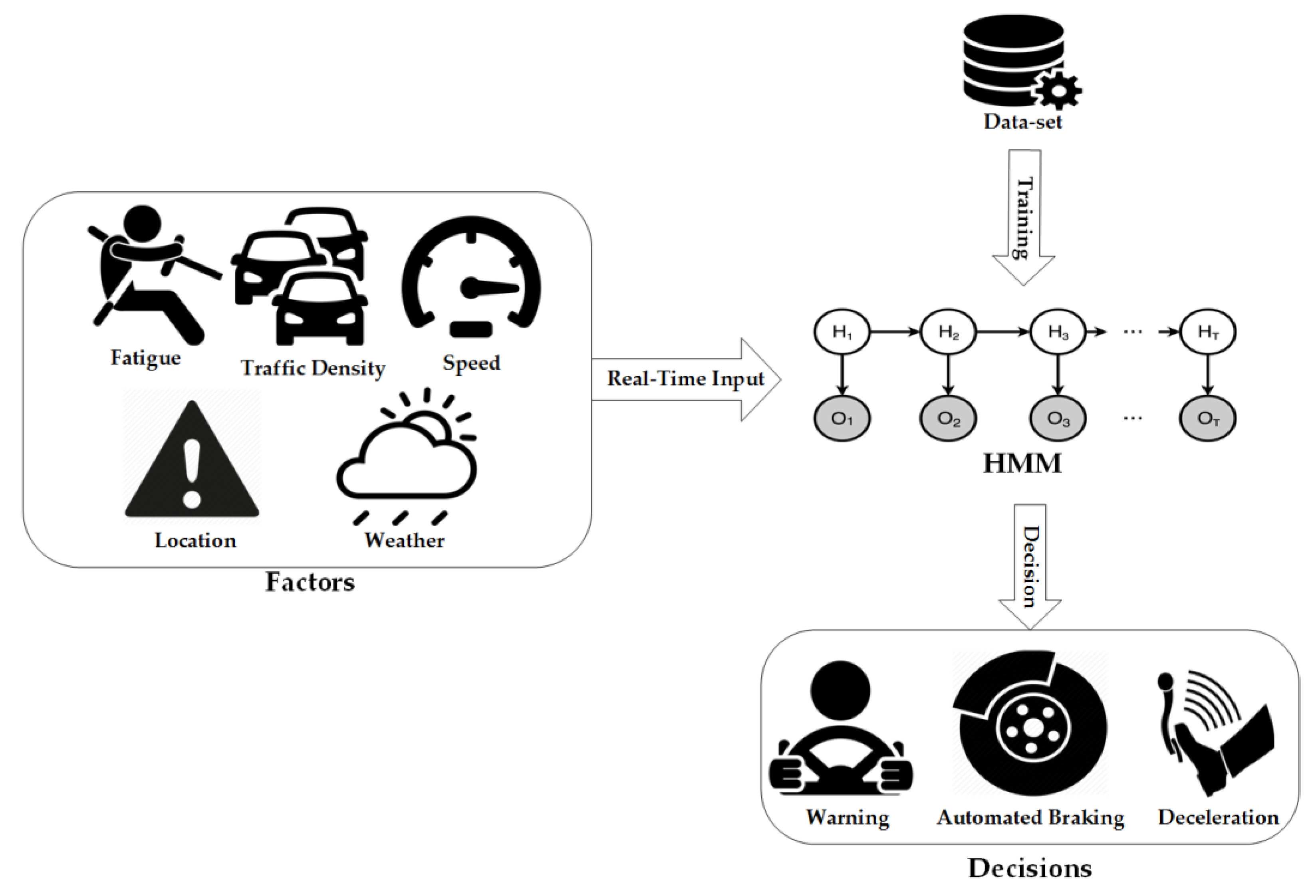
- We proposed a new APS based on VANET and HMM, in which the crash risk was considered as a latent variable.
- Unlike other schemes, besides the velocity, the proposed system also considere other factors that may cause the crash.
- The proposed system was modeled as a weighted multi-observation layer HMM rather than the conventional signal layer HMM.
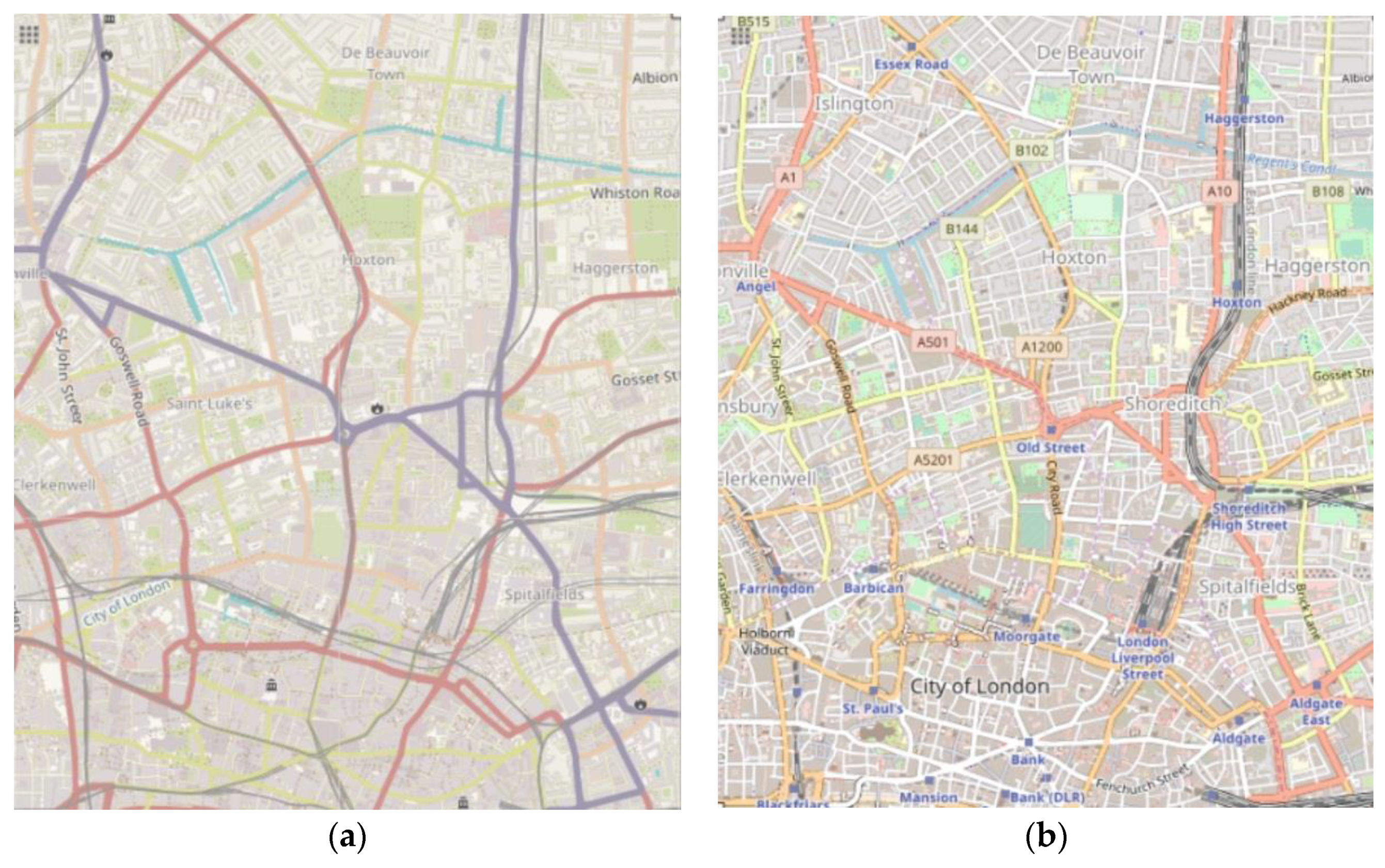
- The proposed system was validated by means of extensive simulation on a map of London city.
- Simulation results showe the high sensitivity and precision of the proposed system.
2. Related Work
2.1. Velocity Based Approaches
2.2. Traffic Density Based Approaches
2.3. Driver Fatigue Based Approaches
2.4. Location Based Approaches
2.5. Weather Based Approaches
3. Preliminaries
3.1. Notations
3.2. Observation Evaluation
3.2.1. Forward Procedure
| Algorithm 1 Forward Procedure |
| for to do end for for to do for to do end for end for |
3.2.2. Backward Procedure
| Algorithm 2 Backward procedure |
| for to do end for for to 1 do for to do end for end for |
4. System Modeling
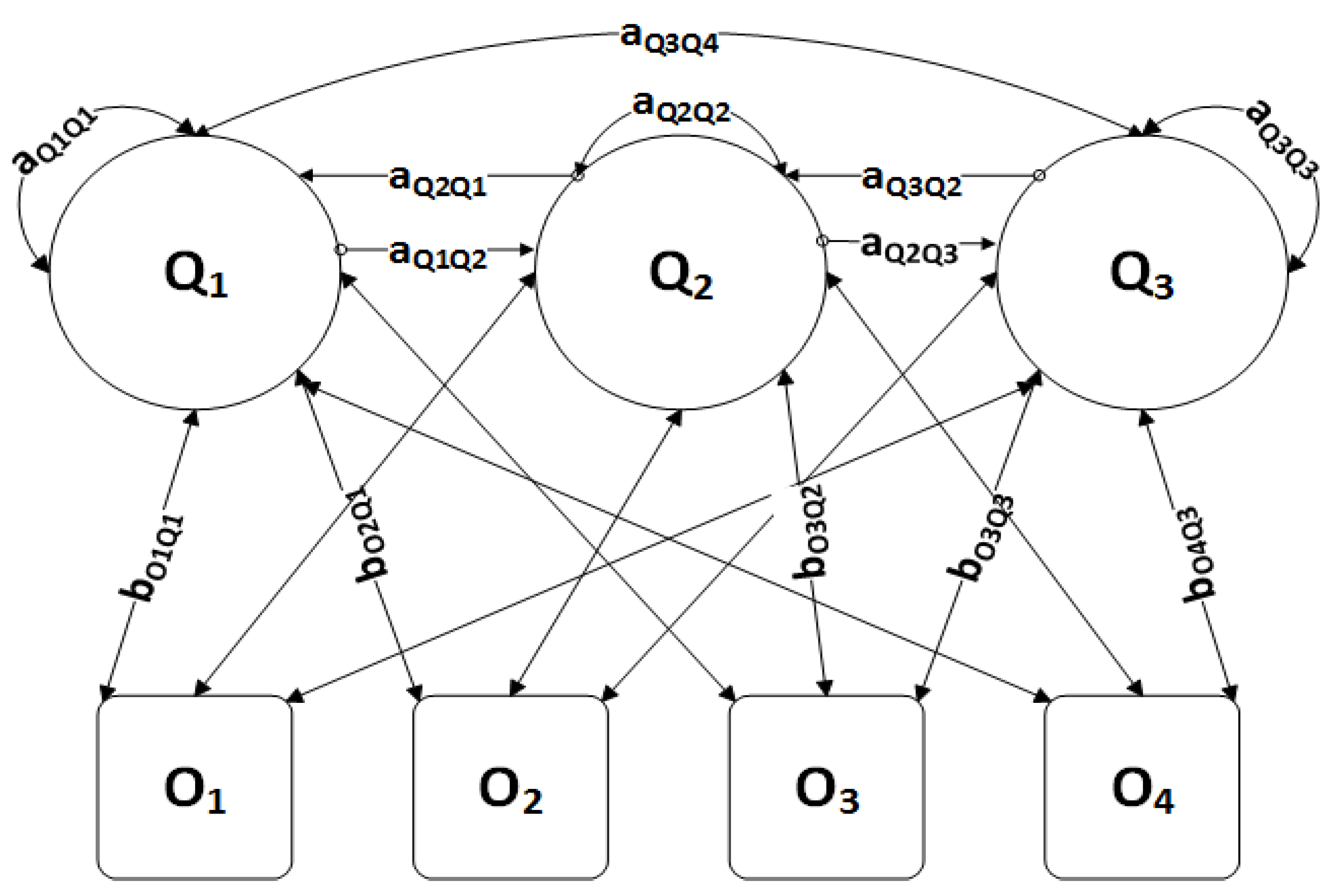
4.1. HMM Parameters
4.2. Probability Fusion
4.3. Training HMM
5. Implementation
5.1. Training Data-Set
- Accident Severity (fatal, serious, slight).
- Accident time (time, date, day of the week,)
- Estimated speed during the accidents
- Whether the road limit was exceeded
- Road speed limit
- Coordinates (Latitude, Longitude)
- Grid reference coordinates (Location Easting OSGR, Location Northing OSGR)
- Weather Conditions (fine no high winds, raining no high winds, snowing no high winds, fine and high winds, raining and high winds, snowing and high winds, fog or mist …etc.)
- Light Conditions (daylight, darkness-lights lit, darkness-lights unlit, darkness-no lighting, darkness-lighting unknown)
- Road surface (dry, wet or damp, snow, frost or ice, flood over 3cm’ deep’, oil or diesel, mud)
- Road Type (roundabout, dual carriageway…etc.)
- Driver’s age
- Journey purpose of driver
- Driver blood alcohol level
- Driver’s health condition
- Number of vehicles involved in the accident
- Vehicle type and propulsion code
- Vehicle reference and engine capacity
- Casualty severity
- Casualties ages
- Casualty type
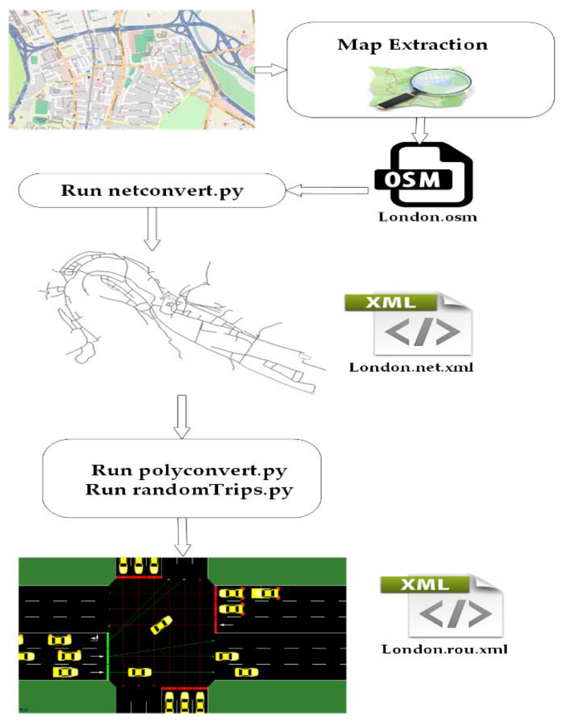
5.2. Simulation Map
5.3. Training the System
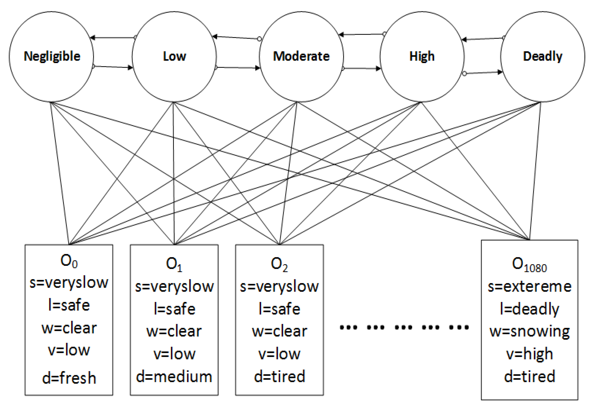
5.3.1. Ranges Mapping
5.3.2. Weights Optimization
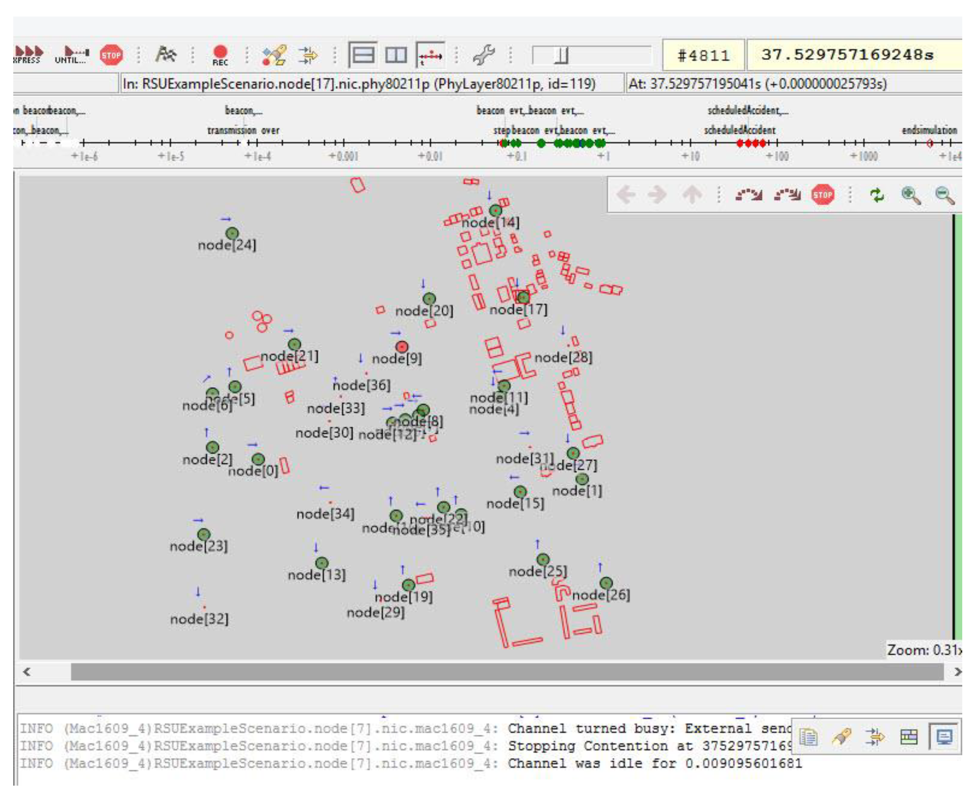
5.4. Traffic Simulation
5.5. V2V Communication Parameters
6. Performance Evaluation
- True positive (TP): the scenario manager launched the crash and the observed vehicle could detect it.
- False positive (FP): the scenario manager did not launch the crash but the observed vehicle falsely detected a crash.
- False negative (FN): the scenario manager launched the crash but the observed vehicle did not detect it.
6.1. Metrics
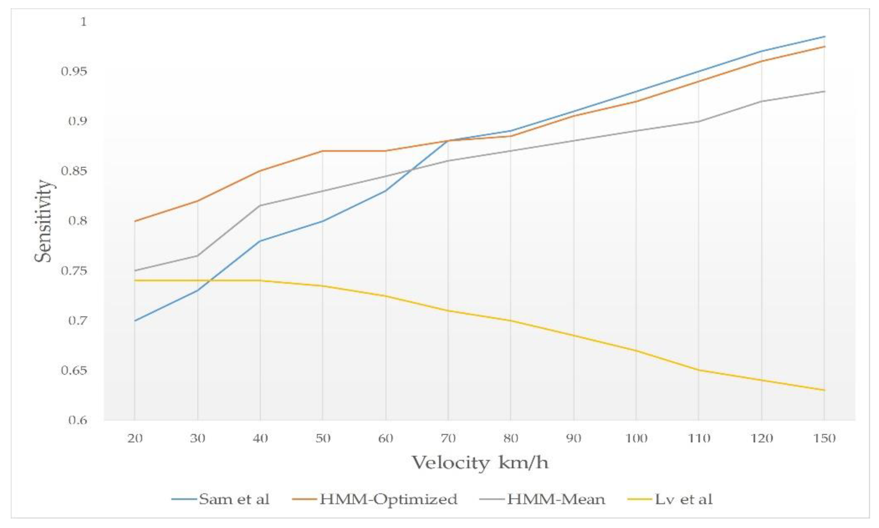
- Velocity vs Sensitivity: in this test, we changed the velocity values to test and compared the sensitivity of the schemes.
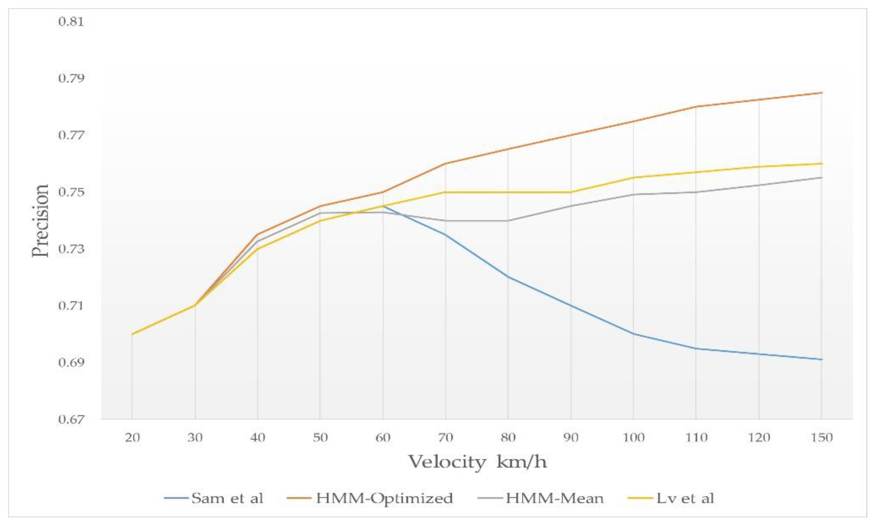
- Velocity vs Precision: in this test, we changed the velocity values to test and compared the precision of the schemes.
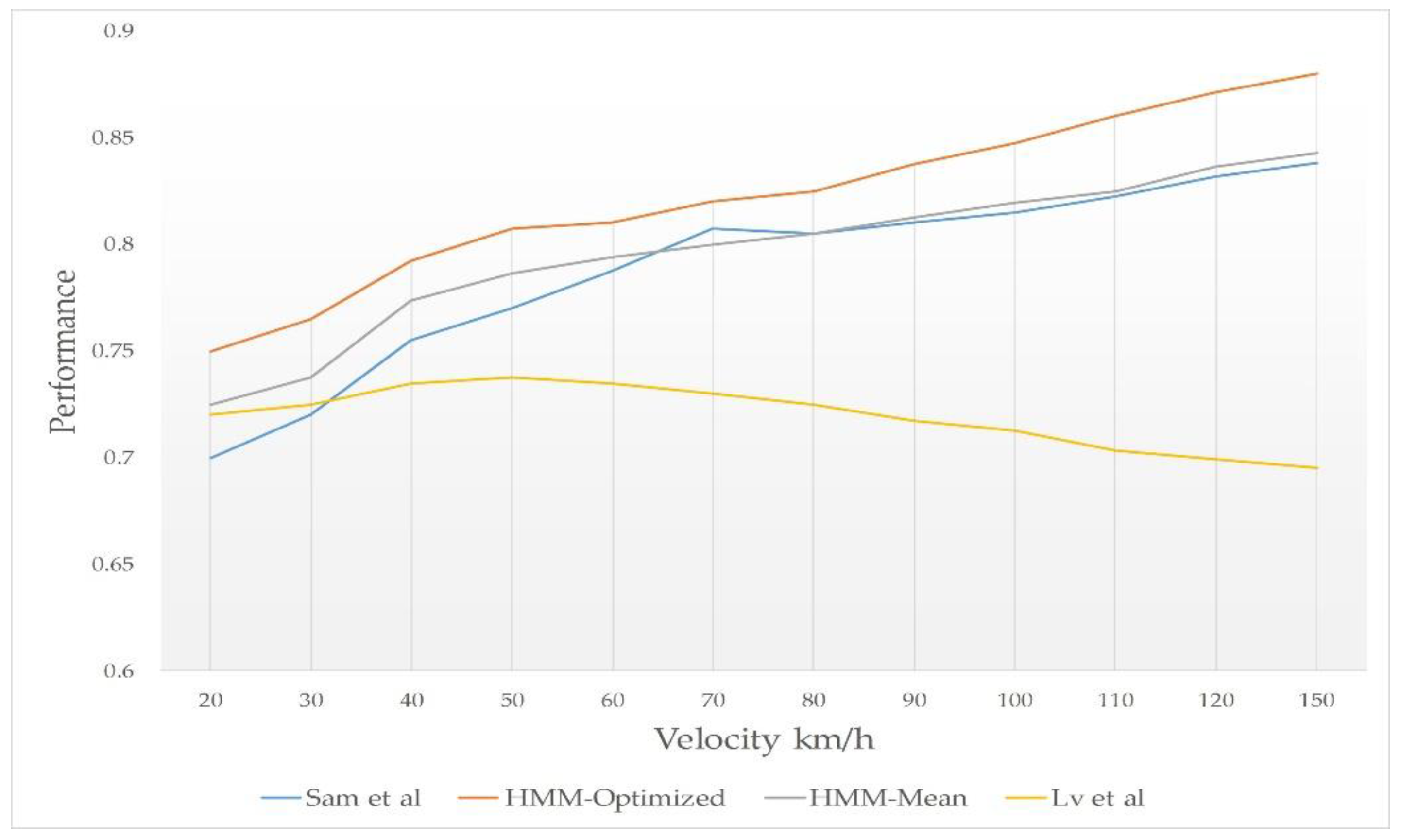
- Velocity vs Performance: to measure the performance of the scheme when changing the velocity value.
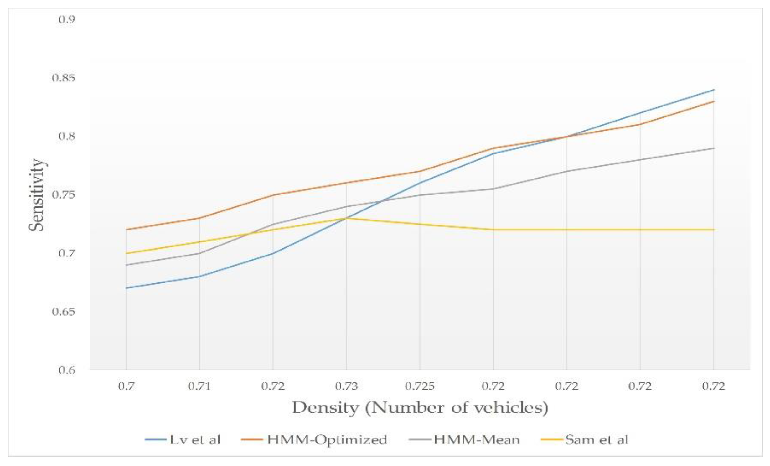
- Density vs Sensitivity: in this test, we changed vehicles density to test and compared the sensitivity of the schemes.
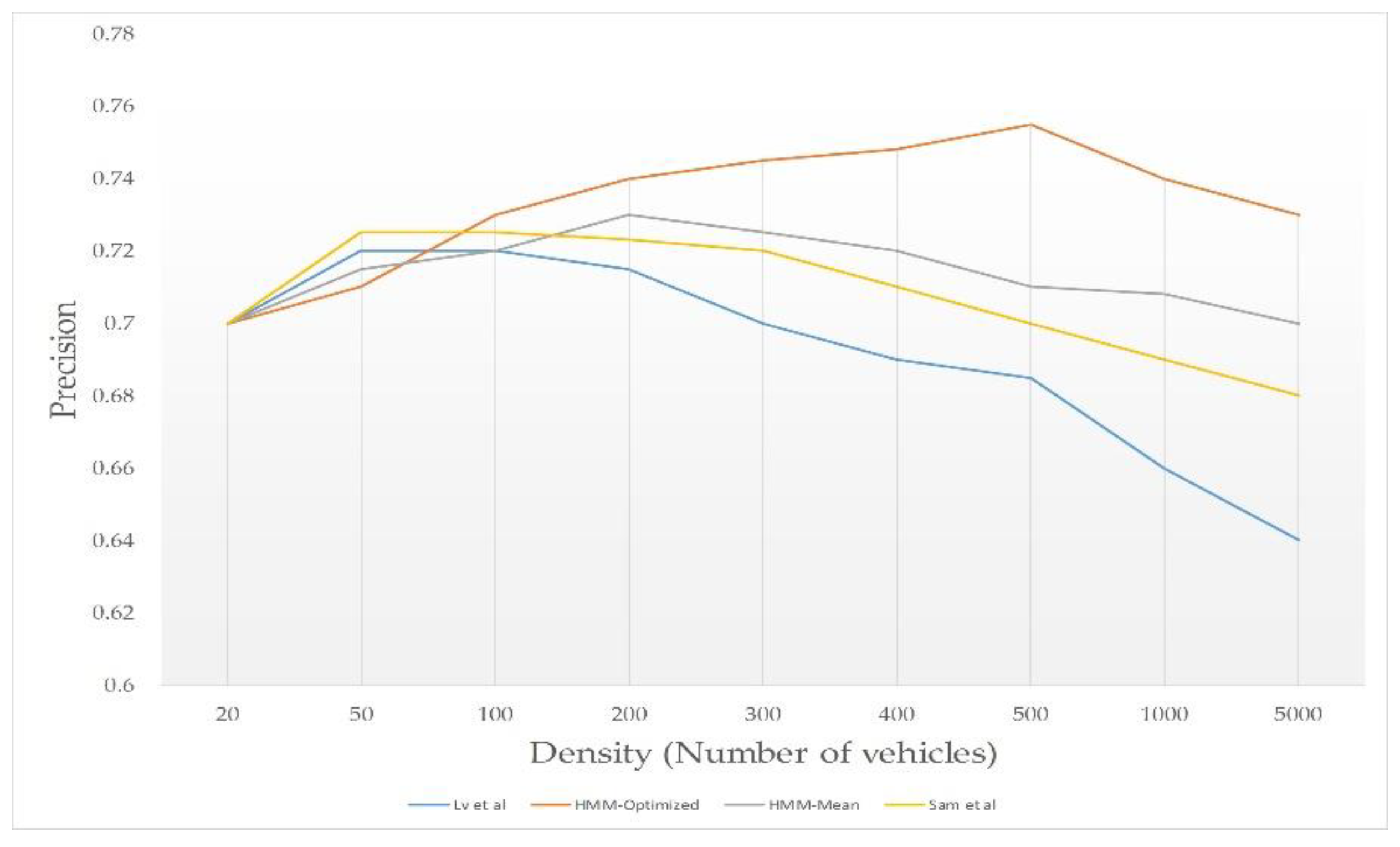
- Density vs Precision: in this test, we changed vehicles density to test and compared the precision of the schemes.
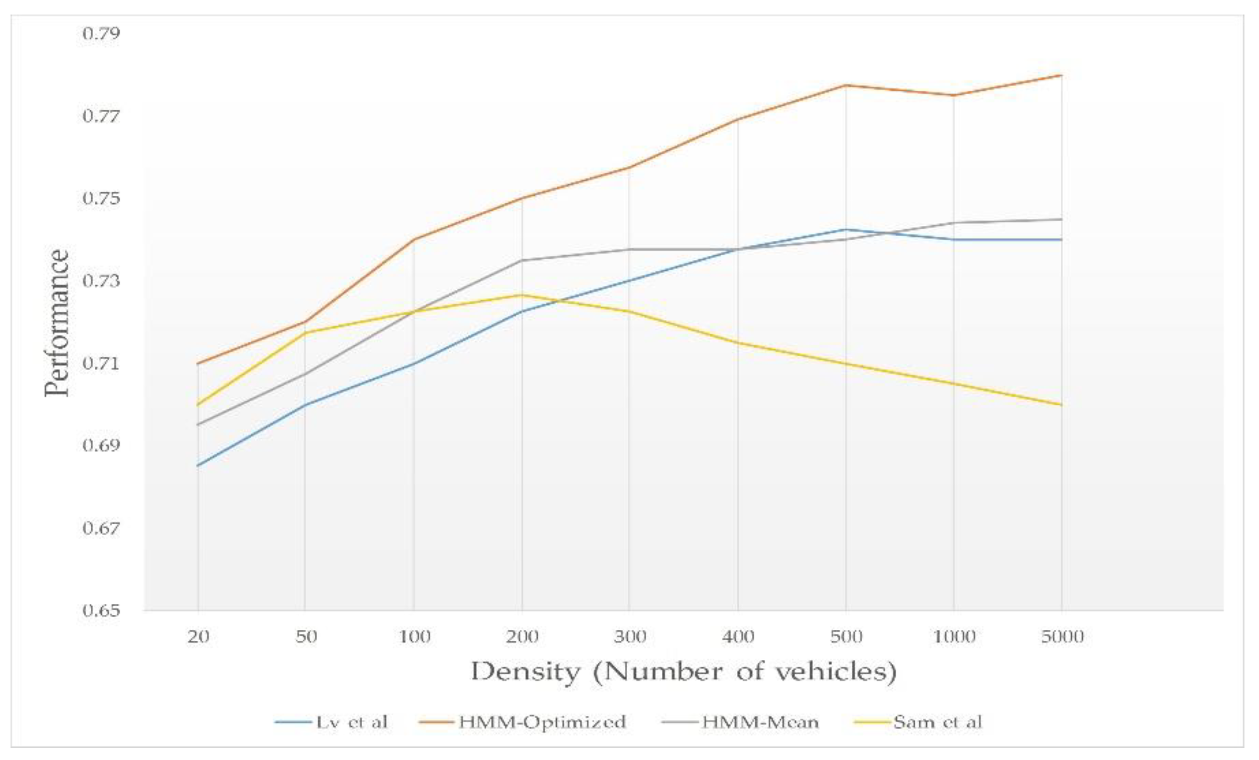
- Density vs Performance: to measure the performance of the schemes when changing the vehicles density.
6.2. Baselines
6.3. Simulation Results
7. Conclusions and Future Directions
Author Contributions
Funding
Acknowledgments
Conflicts of Interest
References
- World Health Organization. Global Status Report on Road Safety: Supporting a Decade of Action; World Health Organization: Geneva, Switzerland, 2013. [Google Scholar]
- WHO Road Traffic Injuries. Available online: http://www.who.int/news-room/fact-sheets/detail/road-traffic-injuries (accessed on 24 November 2018).
- Jing, P.; Huang, H.; Chen, L. An Adaptive Traffic Signal Control in a Connected Vehicle Environment: A Systematic Review. Information 2017, 8, 101. [Google Scholar] [CrossRef]
- Zhang, W.; Aung, N.; Dhelim, S.; Ai, Y. DIFTOS: A Distributed Infrastructure-Free Traffic Optimization System Based on Vehicular Ad Hoc Networks for Urban Environments. Sensors 2018, 18, 2567. [Google Scholar] [CrossRef] [PubMed]
- Hartenstein, H.; Laberteaux, K.P. A tutorial survey on vehicular ad hoc networks. IEEE Commun. Mag. 2008, 46, 164–171. [Google Scholar] [CrossRef]
- Chin, H.C.; Quddus, M.A. Applying the random effect negative binomial model to examine traffic accident occurrence at signalized intersections. Accid. Anal. Prev. 2003, 35, 253–259. [Google Scholar] [CrossRef]
- Lord, D.; Persaud, B. Accident prediction models with and without trend: Application of the generalized estimating equations procedure. Transp. Res. Rec. J. Transp. Res. Board 2000, 102–108. [Google Scholar] [CrossRef]
- Poch, M.; Mannering, F. Negative binomial analysis of intersection-accident frequencies. J. Transp. Eng. 1996, 122, 105–113. [Google Scholar] [CrossRef]
- Mukhtar, A.; Xia, L.; Tang, T.B. Vehicle Detection Techniques for Collision Avoidance Systems: A Review. IEEE Trans. Intell. Transp. Syst. 2015, 16, 2318–2338. [Google Scholar] [CrossRef]
- Kumar, K.P.; Evangelin, S.J.; Amudharani, V.; Inbavalli, P.; Suganya, R.; Prabu, U. Survey on Collision Avoidance in VANET. In Proceedings of the 2015 International Conference on Advanced Research in Computer Science Engineering & Technology (ICARCSET 2015)—ICARCSET ’15, Eluru, India, 6–7 March 2015; ACM Press: New York, NY, USA, 2015; pp. 1–5. [Google Scholar]
- Raut, S.B.; Malik, L.G. Survey on vehicle collision prediction in VANET. In Proceedings of the IEEE International Conference on Computational Intelligence and Computing Research (ICCIC), Coimbatore, India, 18–20 December 2014; pp. 735–751. [Google Scholar] [CrossRef]
- Sam, D.; Velanganni, C.; Evangelin, T.E. A vehicle control system using a time synchronized Hybrid VANET to reduce road accidents caused by human error. Veh. Commun. 2016, 6, 17–28. [Google Scholar] [CrossRef]
- Sharma, B.; Katiyar, V.K.; Kumar, K. Kranti Kumar Traffic Accident Prediction Model Using Support Vector Machines with Gaussian Kernel. In Proceedings of Fifth International Conference on Soft Computing for Problem Solving; Pant, M., Deep, K., Bansal, J.C., Nagar, A., Das, K.N., Eds.; Springer: Singapore, 2016; pp. 1–10. ISBN 978-981-10-0451-3. [Google Scholar]
- Wu, Q.; Hui, L.C.K.; Yeung, C.Y.; Chim, T.W. Early car collision prediction in VANET. In International Conference on Connected Vehicles and Expo (ICCVE); IEEE: Shenzhen, China, 2015; pp. 19–23. [Google Scholar]
- Lv, H.; Xu, P.; Chen, H.; Zhou, B.; Ren, T.; Chen, Y. A novel rear-end collision warning algorithm in VANET. In Proceedings of the 8th IEEE International Conference on Communication Software and Networks (ICCSN), Beijing, China, 4–6 June 2016; IEEE: Beijing, China, 2016; pp. 4–6. [Google Scholar]
- Iqbal, A.; Busso, C.; Gans, N.R. Adjacent Vehicle Collision Warning System using Image Sensor and Inertial Measurement Unit. In Proceedings of the 2015 ACM on International Conference on Multimodal Interaction—ICMI ’15, Seattle, WA, USA, 9–13 November 2015; ACM Press: New York, NY, USA, 2015; pp. 291–298. [Google Scholar]
- Al Najada, H.; Mahgoub, I. Anticipation and alert system of congestion and accidents in VANET using Big Data analysis for Intelligent Transportation Systems. In Proceedings of the IEEE Symposium Series on Computational Intelligence 2016 (SSCI), Athens, Greece, 6–9 December 2016; IEEE: Athens, Greece, 2016; pp. 6–9. [Google Scholar]
- Arbabzadeh, N.; Jafari, M. A Data-Driven Approach for Driving Safety Risk Prediction Using Driver Behavior and Roadway Information Data. IEEE Trans. Intell. Transp. Syst. 2018, 19, 446–460. [Google Scholar] [CrossRef]
- Wang, H.; Dragomir, A.; Abbasi, N.I.; Li, J.; Thakor, N.V.; Bezerianos, A. A novel real-time driving fatigue detection system based on wireless dry EEG. Cogn. Neurodyn. 2018, 1–12. [Google Scholar] [CrossRef] [PubMed]
- Ba, Y.; Zhang, W.; Wang, Q.; Zhou, R.; Ren, C. Crash prediction with behavioral and physiological features for advanced vehicle collision avoidance system. Transp. Res. Part C Emerg. Technol. 2017, 74, 22–33. [Google Scholar] [CrossRef]
- Maile, M.; Chen, Q.; Brown, G.; Delgrossi, L. Intersection Collision Avoidance: From Driver Alerts to Vehicle Control. In Proceedings of the IEEE 81st Vehicular Technology Conference 2015 (VTC Spring), Glasgow, UK, 11–14 May 2015; IEEE: Glasgow, UK, 2015; pp. 11–14. [Google Scholar]
- Akhil, M.; Vasudevan, N.; Ramanadhan, U.; Devassy, A.; Krishnaswamy, D.; Ramachandran, A. Collision avoidance at intersections using vehicle detectors and smartphones. In Proceedings of the International Conference on Connected Vehicles and Expo 2015 (ICCVE), Shenzhen, China, 19–23 October 2015; IEEE: Shenzhen, China, 2015; pp. 19–23. [Google Scholar]
- Bordel, B.; Alcarria, R.; Rizzo, G.; Jara, A. Creating Predictive Models for Forecasting the Accident Rate in Mountain Roads Using VANETs. In Proceedings of the International Conference on Information Technology & Systems (ICITS 2018); Rocha, Á., Guarda, T., Eds.; Springer International Publishing: Cham, Switzerland, 2018; pp. 319–329. ISBN 978-3-319-73450-7. [Google Scholar]
- Wenqi, L.; Dongyu, L.; Menghua, Y. A model of traffic accident prediction based on convolutional neural network. In Proceedings of the 2nd IEEE International Conference on Intelligent Transportation Engineering, ICITE 2017, Singapore, 1–3 September 2017; pp. 198–202. [Google Scholar]
- Zhang, J.; Wang, F.; Zhong, Z.; Wang, S. Continuous Phase Modulation Classification via Baum-Welch Algorithm. IEEE Commun. Lett. 2018, 22, 1390–1393. [Google Scholar] [CrossRef]
- UK Department for Transport Road Safety Data. Available online: https://data.gov.uk/dataset/cb7ae6f0-4be6-4935-9277-47e5ce24a11f/road-safety-data (accessed on 23 November 2018).
- Haklay, M.; Weber, P. OpenStreetMap: User-Generated Street Maps. IEEE Pervasive Comput. 2008, 7, 12–18. [Google Scholar] [CrossRef]
- Behrisch, M.; Bieker, L.; Erdmann, J.; Krajzewicz, D. Sumo-simulation of urban mobility. In Proceedings of the Third International Conference on Advances in System Simulation (SIMUL 2011), Barcelona, Spain, 23–28 October 2011; Volume 42. [Google Scholar]
- Wegener, A.; Piórkowski Michałand Raya, M.; Hellbrück, H.; Fischer, S.; Hubaux, J.-P. TraCI: An interface for coupling road traffic and network simulators. In Proceedings of the 11th Communications and Networking Simulation Symposium, Ottawa, ON, Canada, 14–17 April 2008; pp. 155–163. [Google Scholar]
- Varga, A.; Hornig, R. An overview of the OMNeT++ simulation environment. In Proceedings of the 1st International Conference on Simulation Tools and Techniques for Communications, Networks and Systems & Workshops, Marseille, France, 3–7 March 2008; p. 60. [Google Scholar]


| Symbol | Description |
|---|---|
| Initial state distribution | |
| State transition probability matrix (transition matrix) | |
| The probability of being in state at the time and transfer to state at the time | |
| Observation probability matrix (emission matrix) | |
| The probability of being in state during the observation | |
| The HMM parameters | |
| The observed sequence | |
| Length of the observation sequence | |
| Number of states in the model | |
| Number of observations |
| Factor | Value Range |
|---|---|
| States | Negligible, Low, Moderate, High, Very high, Deadly |
| S | Very Slow, Slow, Medium, High, Very high, Extreme |
| L | Safe, Normal, Dangerous, Deadly |
| W | Clear, Sunny, Rainy, Foggy, Snowing |
| V | Low, Medium, High |
| D | Fresh, Medium, Tired |
| Factor (Reason) | Weight (Percentage) |
|---|---|
| Vehicle speed (WS) | 48.3% |
| Location dangerous level (WL) | 12.9% |
| Weather conditions (WW) | 18% |
| Vehicle density (WV) | 15.8% |
| Driver fatigue (WD) | 5% |
| Parameters | Description |
|---|---|
| Network Simulator | Omnet++ 5 [30] |
| Traffic Simulator | Sumo 0.27.1 [28] |
| Map Information | Openstreetmap [27] |
| Simulated Location | London |
| Simulated area | 3X4 km |
| Parameter | Value |
|---|---|
| PHY model | 802.11 p |
| Channel frequency | 5.890e9 Hz |
| Propagation model | Two ray model |
| MAC model | EDCA |
| Propagation distance | 150 m |
| Maximum hop count | 10 |
| Fading model | Jakes model rayleigh fading |
| Shadowing model | LogNormal |
| Antenna model | Omnidirectional |
| Transmission power | 20 mW |
© 2018 by the authors. Licensee MDPI, Basel, Switzerland. This article is an open access article distributed under the terms and conditions of the Creative Commons Attribution (CC BY) license (http://creativecommons.org/licenses/by/4.0/).
Share and Cite
Aung, N.; Zhang, W.; Dhelim, S.; Ai, Y. Accident Prediction System Based on Hidden Markov Model for Vehicular Ad-Hoc Network in Urban Environments. Information 2018, 9, 311. https://doi.org/10.3390/info9120311
Aung N, Zhang W, Dhelim S, Ai Y. Accident Prediction System Based on Hidden Markov Model for Vehicular Ad-Hoc Network in Urban Environments. Information. 2018; 9(12):311. https://doi.org/10.3390/info9120311
Chicago/Turabian StyleAung, Nyothiri, Weidong Zhang, Sahraoui Dhelim, and Yibo Ai. 2018. "Accident Prediction System Based on Hidden Markov Model for Vehicular Ad-Hoc Network in Urban Environments" Information 9, no. 12: 311. https://doi.org/10.3390/info9120311
APA StyleAung, N., Zhang, W., Dhelim, S., & Ai, Y. (2018). Accident Prediction System Based on Hidden Markov Model for Vehicular Ad-Hoc Network in Urban Environments. Information, 9(12), 311. https://doi.org/10.3390/info9120311