Abstract
Vector geographic data play an important role in location information services. Digital watermarking has been widely used in protecting vector geographic data from being easily duplicated by digital forensics. Because the production and application of vector geographic data refer to many units and departments, the demand for multiple watermarking technology is increasing. However, multiple watermarking algorithm for vector geographic data draw less attention, and there are many urgent problems to be solved. Therefore, an efficient robust multiple watermark algorithm for vector geographic data is proposed in this paper. The coordinates in vector geographic data are first randomly divided into non-repetitive sets. The multiple watermarks are then embedded into the different sets. In watermark detection correlation, the Lindeberg theory is used to build a detection model and to confirm the detection threshold. Finally, experiments are made in order to demonstrate the detection algorithm, and to test its robustness against common attacks, especially against cropping attacks. The experimental results show that the proposed algorithm is robust against the deletion of vertices, addition of vertices, compression, and cropping attacks. Moreover, the proposed detection algorithm is compatible with single watermarking detection algorithms, and it has good performance in terms of detection efficiency.
1. Introduction
Vector geographic data are very important basic and strategic national information resources, which play a significant role in fields referring to location information. The safety of vector geographic data is closed in terms of public and individual security. With the advent of the informational era, it has become much easier to acquire, transmit, and distribute vector geographic data. Security problems have become increasingly prominent. Furthermore, the protection demands of multiple users and multi-copyright for vector geographic data that are caused by multi-level transmission are becoming increasingly urgent. It is currently necessary to focus on how to effectively protect the multi-copyrights of vector geographic data and how to track multiple users. Multiple watermarking technology involves the embedding of multiple watermarks into the cover data. It can be used to protect the copyrights of multiple users, and to track the copying flow of data in the progress of multi-level transmission. Therefore, multiple watermarking technology can effectively solve the above information security problems of vector geographic data.
Currently, many scholars have been devoted to developing digital watermark technology, and they have proposed many algorithms [,,,,,,,,,,,,,,,]. However, these algorithms focus on embedding only one watermark in the cover data, which then lacks multi-copyright protection. Multiple watermarking draws less attention than single watermarking, and it does not simply involve the embedding of different watermarks by using the single watermarking algorithm. The multiple watermarking algorithm commonly focuses on images and videos. There are three main methods for addressing the impact of multiple watermarks, as described in References [,,,,,,,,,,,,,]. The first is dividing the images into multiple blocks for multiple watermarks [,,,]. The second is embedding multiple watermarks into different frequency domains or channels [,,,,,,]. The last is merging multiple watermarks into one [,,]. Usually multiple methods are combined in one algorithm. In the above references, only a few previous works have been proposed for vector geographic data; for instance, References [,,,,,]. Sun et al. combined a child copyright watermark with another child watermark consisting of features selected by fuzzy clustering from the vector map. The new watermark was then embedded into the vector map []. Li et al. proposed a multiple watermark embedding solution through the generation of additional information with watermark embedding []. Zhang et al. embedded two watermarks into a spatial domain and transform domain in turn []. Cui proposed three multiple watermarking algorithms for vector geographic data in his doctorate dissertation []. The first method embeds the two watermarks into the X and Y coordinates separately. The second method joins multiple watermarks as one and uses the single watermarking algorithm to embed the composed watermark. These two methods require the number of watermarks in advance. The third method involves the division of the vector geographic data into blocks based on a quad-tree algorithm and embeds the multiple watermarks into different blocks. Wang proposed a non-blind multiple watermarking algorithm that embedded multiple watermark bits into the same vertices, according to an adding method []. The watermark capacity is improved and robust against common watermark attacks, but the original data is necessary in the detection process. To overcome this restriction, Wang proposed a multiple watermarking algorithm for vector geographic data, based on coordinate mapping and domain subdivision []. Before embedding the watermarks, the method of dividing blocks has been improved to protect against cropping attacks.
The digital watermarking algorithms based on simple block and sequence division are weak against cropping attacks, which are frequent in vector geographic data processing. Furthermore, the original maps and the embedding locations of watermarks are absent in actual use, and hence the robustness and detection algorithm of multiple watermarking urgently needs to be improved. Aiming at convenient multiple watermark detection and at preserving all watermarks in the watermarked data after cropping attacks, a multiple watermarking algorithm against cropping attacks for vector geographic data is proposed in this paper. The vertices in the vector geographic data are randomly divided into different vertex sets. Multiple watermarks are embedded into corresponding vertex sets. Since the watermark bits are randomly embedded into vertices, the watermarks are difficult to be removed when the data are cropped. In the watermark detection process, the detection model is built based on the different probability distribution characteristics of the watermark and according to whether there is a certain watermark or not. The detection threshold is obtained according to correlation detection, based on the Lindeberg Theory. Thus, the watermarks are extracted as a whole, and then they are distinguished from each other without the help of the original data.
The remaining sections are organized as follows. Section 2 presents the blind multiple digital watermarking algorithm, and demonstrates the applicability of the proposed watermark detection algorithm. Section 3 provides the experimental results of the algorithm. The conclusions are summarized in Section 4.
2. The Multiple Watermarking Algorithm
The traditional watermark algorithm includes three parts: watermark generation, watermark embedding, and watermark detecting, as seen in Figure 1. In the distribution and transportation process of the watermarked map, it is usual to delete vertices, add vertices, compress data, and crop the map. These operations change the map, and they may break the watermark, which are considered as watermark attacks. The ability of the watermarking algorithm to withstand against watermark attacks is its degree of robustness. As a multiple watermarking algorithm, the proposed algorithm is similar to the traditional algorithm, but watermark embedding and detection are different. The entire procedure of the proposed algorithm is shown in Figure 2. In the watermark embedding stage, multiple watermarks are embedded, and these watermarks need to be detected in the watermark detection program. The specific procedures are stated in this section.
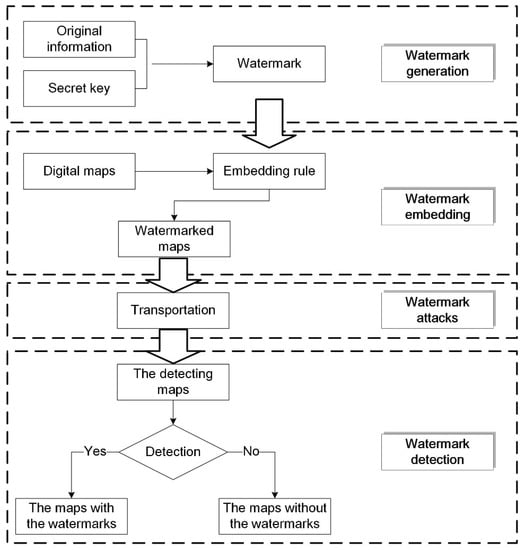
Figure 1.
The traditional watermark algorithm.
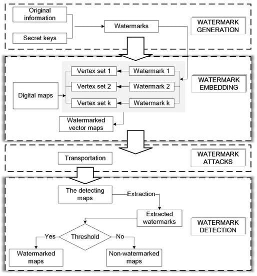
Figure 2.
The proposed multiple watermarking algorithm.
2.1. Watermark Generation
Watermarks can be categorized into two classifications: meaningful and meaningless watermarks. Meaningful watermarks have explicit meanings, such as voice, video, images, characters, etc., while meaningless watermarks do not usually have explicit meanings; for example, pseudorandom and chaotic sequences. Generally, the length of a meaningless watermark is longer than a meaningful watermark. For meaningless watermarks, the watermark should be extracted before watermark detection. This section represents the proposed multiple watermark algorithm in this flow. Figure 2 shows the flow of the proposed algorithm. Considering the data size of the vector geographic data, the numbers of watermarks, and the statistical characteristics, a meaningless watermark with a pseudorandom binary sequence was used in the proposed algorithm.
The different watermarks were generated by using a pseudorandom binary sequence generator. Let the watermark be , where is the length of the watermark, and is the index of the watermark bit, as shown in Figure 3. Also, the bits , where either value is equally likely; the probabilities are and . Taking vector geographic data with a small data size into account, should not be too large, and thus in our experiments.
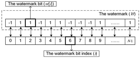
Figure 3.
The relationship between the watermark, the watermark bits, and the watermark bit indices.
In the proposed algorithm, let the th watermark be , where is the th watermark bit index of the th watermark, and . There is no correlation between any two watermarks and . When , . When , is close to . In general, ; the normalized correlation detection value obeys a normal distribution with a mean of 0, and a variance of .
2.2. Watermark Embedding
In vector geographic data processing, adding vertices, deleting vertices, data compression, and cropping are common. The watermarks may be removed in the above processes, which are considered to be watermark attacks. There is an urgent need for robust watermarks that can be preserved and detected after these common attacks.
Considering this problem, for a single watermark, coordinate mapping and quantization are used in watermark embedding. The basic idea is that a “one-to-many” relationship between the watermark bit indices and the vertices is established [], and then the watermark bit is embedded in the coordinates repeatedly by using quantization []. The embedding model is shown in Equation (1):
where is the vertices set, is the th coordinate in the set, is the embedding rule, is the mapping relationship between vertices and the watermark bit indices, which satisfies . should ensure that the vertices are evenly mapped to the watermark bit index of each watermark.
Considering multiple watermarks and the vertices set, is first randomly divided into multiple subsets. If there are watermarks being embedded, is divided into non-repetitive subsets, and . Let there be vertices in and vertices in , so . Figure 4 shows one example where the vertices in the digital map are randomly divided into three subsets. The different color points represent different vertex sets. To improve robustness against cropping attacks, in the process of division, the data size of is decided by the number of the watermarks. Based on Equation (1), multiple watermarks are embedded by using the rule shown in Equation (2) (the flowchart of multiple watermarks being embedded is shown in Figure 5):
where is the th coordinate in the vertex subset and .
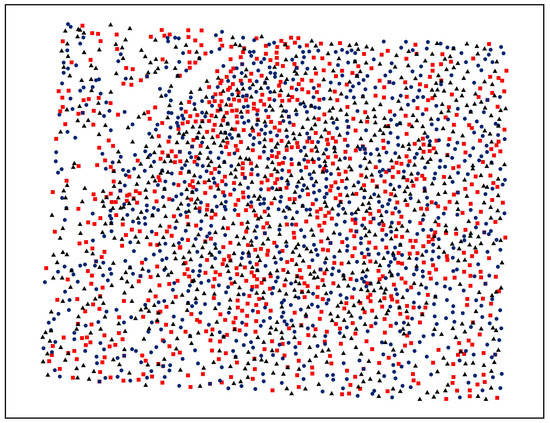
Figure 4.
An example of dividing data using three non-repetitive vertex sets.
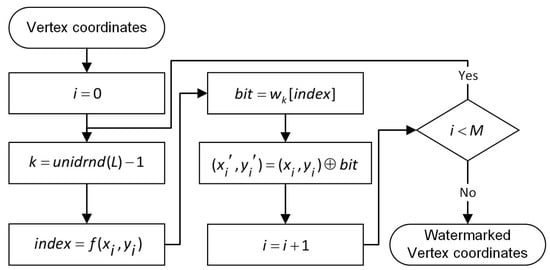
Figure 5.
The flowchart of multiple watermark embedding. unidrnd() returns random numbers chosen uniformly from the set .
2.3. Watermark Extraction and Detection
2.3.1. Watermark Extraction
Detection of a meaningless watermark concludes the process of watermark extraction and detection. In watermark extraction, the watermark bit sets are extracted from the data. The flowchart of multiple watermark extraction and detection is presented in Figure 6.
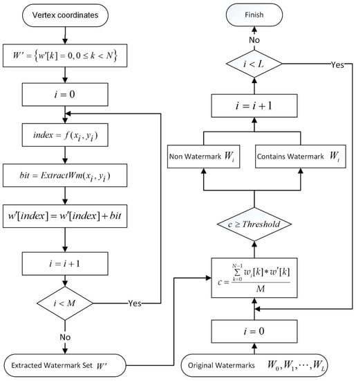
Figure 6.
The flowchart of multiple watermark extraction and detection.
The watermark extraction is the inverse process of watermark embedding. The following basic procedure is used. The watermark bits in the arbitrary vertices are extracted according to the embedded quantization step. The watermark is then mapped onto the correlated watermark bit indices according to the mapping relationship. These steps are repeated, and the watermark bit set is extracted in all vertices. In most cases of watermark extraction, the data size of the carried data is much more than the length of the watermark, . Hence, the same watermark bit index corresponds to many extracted watermark bits.
For the usual process of watermark extraction and detection, the vertex set, , first needs to be rebuilt according to the watermarked data. However, it is difficult to rebuild the vertex set because of potential watermark attacks in data processing, such as deleting vertices, adding vertices, data compression, and data cropping. Hence, the proposed algorithm considers the watermarked data in its entirety for watermark extraction, and correlation detection is adopted in watermark detection to distinguish the different watermarks.
Let the extracted watermark bits set be . and , where is the th watermark bit corresponding to the extracted watermark index and .
2.3.2. Watermark Detection
Let the correlation detection statistic be for detecting , as shown in Equation (3). The probability distribution of is different when if there are watermarks in the cover data as opposed to when no watermarks are present. The following are the specific conditions for different situations:
1. There is no watermark in the cover data
If there is no watermark in the cover data, it is random for the extracted watermark bit to be equal to −1 or 1, that is, , , so that obeys the probability distribution of Equation (4):
2. There are watermarks in the cover data
There are two possibilities in this situation. One is that there is a specific watermark in the extracted watermark bits set, and the other is that watermark is not present. Let be the summation of the extracted watermark bits corresponding to the watermark bit index , which is presented in Equation (5):
There may be multiple watermarks in the cover data; consists of two parts: the watermark bits of and the watermark bits corresponding to other watermarks. Equation (6) presents this relationship:
where is the summation of watermark bits corresponding to , and is the summation of watermark bits corresponding to the other watermarks. Equation (7) shows the corresponding detection:
For the watermarked data, the distribution characteristics of are discussed in two situations as follows.
● There is no in the watermarked data
In this situation, , , and Equation (3) is equal to the following:
Because and , obeys the distribution and . According to the Lindeberg theory, obeys the normal distribution shown in Equation (9) when the Lindeberg conditions are satisfied:
● There is in the watermarked data
In this situation, , and Equation (3) is equal to the following:
The watermark, , is embedded in vertices; hence, Equation (10) can be simplified to:
Similarly, according to the Lindeberg theory, obeys the normal distribution that is shown in Equation (12) when the Lindeberg conditions are satisfied:
In conclusion, Equations (9) and (12) show the probability distribution of when is absent and present in the cover data, respectively. Additionally, Equation (3) is one of the special situations for Equation (9).
According to Equations (9) and (12), in multiple watermark detection processes, the detection threshold can be calculated based on the different probability distributions of . The following are the specific steps to calculate the detection threshold in the two conditions.
1. The discriminant analysis is used to calculate the detection threshold when is known.
Mahalanobis distance discrimination analysis can be adopted to build a watermark detection model if is embedded in the vertices whose numbers and spatial distribution are known. Let the distributed population for Equation (9) be , and the distributed population for Equation (12) be . The Mahalanobis distance of the correlation coefficient to and can be depicted as shown in Equations (13) and (14):
When , according to the Mahalanobis distance discrimination analysis, the discriminant function used to detect the watermark can be illustrated as shown in Equation (15):
The detection threshold is , and the watermark detection rule is shown in Equation (16):
According to Equations (9), (12), and (15), the false positive error (FPE), , and the false negative error (FNE), , can be calculated via Equation (17):
2. Controlling the false positive error is used to calculate the detection threshold when is unknown.
Generally, the spatial distribution and the numbers of the watermarked vertices are unknown. In this situation, controlling the FPE is adopted to calculate the threshold. The “” principle can be used to calculate the detection threshold. Based on Equation (9), , which means that the FPE is smaller than . Thus, the detection threshold, , can be set to . The FPE and the FNE can then be calculated by the following:
In fact, the number and the spatial distribution of the detected data that contain the watermark, , is difficult to know, so that the detection threshold used in the experiments below is calculated by controlling the false positive error and the “” principle.
2.3.3. Applicability Analysis
Equations (9) and (12) in Section 2.3.2 show the distribution probabilities under two conditions, which is the basis of the detection model. However, the premise for Equations (9) and (12) are the Lindeberg conditions, which are difficult to demonstrate by means of theoretical derivation. In this section, the applicability of this detection model is verified through experiments.
The experiments are made in different digital vector geographic maps in a shapefile format. Figure 7 shows one group of experimental maps. Figure 7a shows a resident map that is organized as points. Figure 7b shows a river map organized as polygons. Figure 7c,d are river maps organized as polylines. Additionally, all of the maps are presented at a scale of 1:1 million and in the unit of the meter.
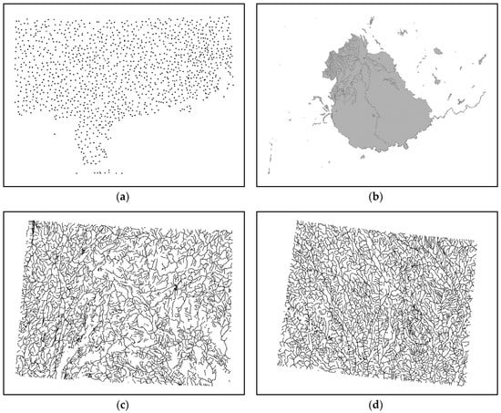
Figure 7.
Examples of experimental data. (a) Digital vector geographic maps organized as points; (b) digital vector geographic maps organized as polygons; (c) and (d) digital vector geographic maps organized as polylines.
In the experiments, two watermarks are embedded in the vector geographic data, and the specific verifying steps are followed.
- (1)
- Randomly divide the vertices in the cover data into two non-repetitive sets.
- (2)
- Generate two watermarks, watermark 1 and watermark 2, and then embed the two watermarks in the two sets.
- (3)
- Extract the watermark, according to Equation (3); the corresponding detection is done by using watermark 1 and watermark 2. The correlation detection coefficients are cor3 and cor4.
- (4)
- Normalize cor3 and cor4 according to Equation (19).
- (5)
- Generate two other watermarks, watermark 3 and watermark 4.
- (6)
- Watermark 3 and watermark 4 are used to carry out the corresponding detection with the extracted watermark according to Equation (3), to obtain the correlation detection coefficients cor1 and cor2.
- (7)
- Normalize cor1 and cor2 according to Equation (20).
- (8)
- Repeat steps (1) to (7) 1000 times and record the experimental results, cor1, cor2, cor3, and cor4.
The experimental data produced 1000 groups of correlation detection coefficients (cor1, cor2, cor3, and cor4). cor1 and cor2 are the detection results when there are no corresponding watermarks in the cover data, and cor3 and cor4 are the detection results when there are corresponding watermarks in the cover data. They should all theoretically obey standard normal distribution.
After the above experiments, 2000 groups of watermark detection values corresponding to every experimental map were created for when there was or was not a corresponding watermark in the cover data. Let the four groups of 2000 values corresponding to the four experimental maps be Data1, Data2, Data3, and Data4, when there are no corresponding watermarks in the detecting maps. Similarly, let the four groups of 2000 values corresponding to the four experimental maps be Data5, Data6, Data7, and Data8, when there are corresponding watermarks.
Hence, verifying the applicability of Equation (9) is equal to analyzing the statistical probabilities of Data1, Data2, Data3, and Data4. Verifying the applicability of Equation (12) is equal to analyzing the statistical probabilities of Data5, Data6, Data7, and Data8. The detection result distribution plot and normal probability plots are drawn, and the means and standard deviations are calculated. The results are shown in Figure 8 and Figure 9 to conveniently analyze the statistical probability. Figure 8 shows the experimental results corresponding to Data1, Data2, Data3, and Data4. Figure 9 shows the experimental results corresponding to Data5, Data6, Data7, and Data8.
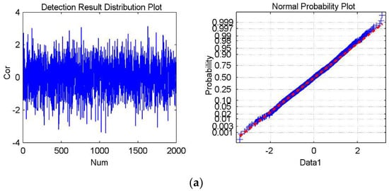
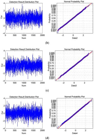
Figure 8.
The experimental results for Watermark3 and Watermark4, which are not present in the cover data. (a–d) shows the detection result distribution plot and the normal probability plot of Data1, Data2, Data3, and Data4, respectively. The mean is 0.00043, and the standard deviation is 1.0128 in (a); the mean is −0.0288, and the standard deviation is 1.0186 in (b); The mean is 0.0105 and the standard deviation is 0.9956 in (c); The mean is −0.0199 and the standard deviation is 1.0003 in (d).
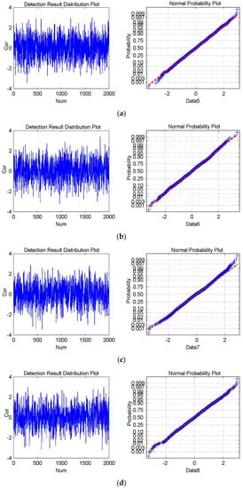
Figure 9.
The experimental results for Watermark1 and Watermark2, which are the cover data. (a–d) shows the detection result distribution plot and the normal probability plot of Data5, Data6, Data7, and Data8, respectively. The mean is −0.0134 and the standard deviation is 0.9969 in (a); the mean is 0.0058 and the standard deviation is 1.0296 in (b); The mean is −0.0284 and the standard deviation is 1.0253 in (c); The mean is −0.0022 and the standard deviation is 1.0144 in (d).
The two figures presenting the experimental results are consistent with the theories that obey the standard normal distribution with a mean of 0 and a variance of 1, which means that the detection model based on Equations (9) and (12) is applicable. Hence, the proposed multiple watermarking detection model can be used to detect multiple watermarks.
3. Experimental Results and Discussion
To verify the performance of the algorithm, the proposed multiple watermarking algorithm was realized by using VC++ 6.0, and the shapefile format data were used for the experiments. Experimental analysis was carried out in a computer environment with Windows 7, Intel Core i5-4200 CPU, and 8.0 GB memory. The robustness, especially against cropping attacks and the efficiency of watermarks detection, was specifically analyzed.
3.1. Robustness Experiments
The robustness experiments involved the detection of watermarks being attacked in the cover data. In order to evaluate the robustness of the proposed multiple watermarking algorithm, experiments were performed on different digital vector geographic maps in a shapefile format. The same experiment steps were repeated for the different vector geographic data. Figure 7 in Section 2.3.3 is an example of experimental data.
The specific robust experimental steps are followed. Generate three watermarks randomly: Watermark1, Watermark2, and Watermark3. Embed Watermark1 and Watermark2 in the experimental data. Attack the watermarked data and detect the three watermarks. In experiments, the attacks included deleting vertices, adding vertices, data compression, and cropping, which are common in data processing for vector geographic data. Table 1 shows the robustness against random deletion attacks, Table 2 shows the robustness against random addition attacks, Table 3 shows the robustness against compression attacks, and Table 4 shows the robustness against cropping attacks. The data size in the tables represents the number of vertices in the detected data. The experimental results in the following tables correspond to the experimental data in Figure 7d.

Table 1.
The detection results after randomly deleting vertices of the experimental data.
Table 2.
The detection results after the random addition of vertices to the experimental data.
Table 3.
The detection results after compression of the experimental data.
Table 4.
The detection results after cropping of the experimental data.
In the robustness experiment, Watermark1 and Watermark2 were embedded into the experimental data. The coordinates being embedded in Watermark1 or Watermark2 were approximately equal and randomly distributed in the data. If the data were not attacked, according to Equation (12), the results of detecting Watermark1 and Watermark2 should follow the normal distribution, with an average value of 0.5, i.e., . The robustness experimental results found detection results of 0.5156 and 0.5102, which were consistent with the above inference. Watermark3 was not embedded into the experimental data, so that according to Equation (9), the results of detecting Watermark3 should follow the normal distribution, with an average value of 0.0, i.e., . In Table 1, Table 2, Table 3 and Table 4, the experimental result for Watermark3, when there was no attack was −0.0156, and the result was close to 0, which was also consistent with the inference.
Deleting vertex attacks involve deleting the vertices in the detecting data randomly, then extracting and detecting the watermarks in the data. Table 1 shows that the detection results of Watermark1 and Watermark2 are close to 0.5, and that they become bigger as the deletion vertices and detection threshold increases. The main reason for this is that Watermark1 and Watermark2 are uniformly and randomly embedded into the cover data. After randomly deleting vertices, the proportion of the number of coordinates containing Watermark1 and Watermark2 in the cover data remains unchanged, i.e., . Watermark1 and Watermark2 are respectively used for watermark detection. According to Equation (12), the relevant detection results should still follow the normal distribution, with a mean value of 0.5. According to the detection threshold calculation formula (), the detection threshold becomes smaller as the number of coordinates in the cover data decrease.
Adding vertex attacks involve adding the vertices in the cover data randomly, then extracting and detecting the watermarks in the data. Table 2 shows the detection results of Watermark1 and Watermark2 are close to 0.5, and that they become smaller as the detection threshold increases. The main reason for this is that the added vertices are not embedded into the watermarks. After randomly adding vertices, the proportion of the number of coordinates containing Watermark1 and Watermark2 in the cover data decreases. That is, decreases. Therefore, according to Equation (12), the detection value corresponding to Watermark1 and Watermark2 will constantly decline. According to the detection threshold calculation formula (), the detection threshold will increase with an increase in the number of coordinates in the cover data.
For the proposed detection algorithm, the data compression and data cropping attacks are similar to randomly deleting vertex attacks. After compression and cropping attacks, the proportion of the coordinates of the embedded watermarks in the cover data remains, and the watermark detection result is close to 0.5. In the following tables, √ shows the watermark can be detected and × shows the watermark can’t be detected.
The same experiments are made on 20 other digital vector maps, which are organized as points, polylines, and polygons. The experiments are in accordance with the above tables. The added vertices, deleted vertices, and cropping in the experiments are all random process. The compression attack used the Douglas–Peucker algorithm, which is classical and common []. The experimental results in the previous tables show that the algorithm is robust against different levels of addition, deletion, compression, and cropping attacks.
3.2. Discussion of Robustness against Cropping Attacks
In this section, experiments have been carried out to compare the robustness against cropping attacks among the proposed algorithm, the third algorithm in Reference [], and the algorithm in Reference []. Four of the same watermarks are embedded in the same experimental maps, based on the three different algorithms, and then the watermarked maps are randomly cropped. The different types of cropping attacks are presented in Figure 10. The full maps are cropped to the various shaded areas shown in Figure 10a–e. Finally, watermarks are detected from the attacked experimental data. The detection results are shown in Table 5.
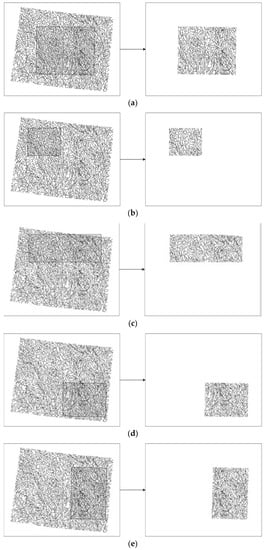
Figure 10.
The different cropping attacks employed in our experiments.
Table 5.
Robustness against cropping attacks for different algorithms.
The algorithm in Reference [] divides the blocks according to the quad-tree method, and the vertices that embed the same watermark may be concentrated in one block. If this block was cropped, the watermark may be removed. The algorithm in Reference [] establishes the logic domains by building the mapping relationship before the subdivision. All of the watermarks were preserved after the cropping attacks. In the proposed algorithm, the vertices were randomly divided into non-repetitive sets in multiple watermark embedding, and the vertices watermarked as the same watermark bit were distributed in the digital map randomly. When one part of the map was cropped, some of the watermark bits were preserved after being cropped. Therefore, the proposed algorithm was robust against cropping attacks.
3.3. Discussion of Detection Efficiency
The detection efficiency is focused upon in this section. In this experiment, four watermarks were embedded into the experimental data using the three different multiple watermarking algorithms, respectively. These watermarks were then detected from the watermarked data, and the detection time was recorded. Six different vector maps were used as experimental data, and the detection efficiency for different algorithms is shown in Table 6.
Table 6.
The detection efficiencies of different algorithms.
The experimental results in Table 6 show that the proposed algorithm had a good level of performance in terms of detection efficiency. The detection time increased with the growth of the number of vertices in the cover data. The detection time of the proposed algorithm was lowest of these three algorithms. The algorithms in References [,] required knowledge of the embedding locations of the watermarks. The different block division methods affected the detection time. The block division based on the quad-tree method was simpler than coordinate mapping and domain subdivision, and so the algorithm in Reference [] spent less time on detection than the algorithm in Reference []. The proposed algorithm extracted the watermarks as an entity, and the embedding location was not necessary in detection.
4. Conclusions
A multiple watermarking algorithm is proposed for vector geographic data, based on the characteristics of the vector geographic data and correlation detection. A multiple watermark embedding algorithm is first designed. Then the detection model is built according to the different probability distribution of watermark detection results; whether there is a watermark in the cover data or not. Meanwhile, the applicability of the detection model is verified through experiments. Finally, experiments are made for evaluating the robustness and detection efficiency. The experimental results show: (1) The proposed algorithm can detect the watermarks directly and efficiently without the necessity of locating the different watermarked vertices. (2) The multiple watermarks are randomly embedded in the cover data, which is useful for increasing the robustness against cropping attacks for the vector geographic data.
In watermark detection, the extracted watermark is considered as a whole, and the multiple watermarks are noise for each other, which is a negative effect on multiple watermarking. In addition, under the condition that there is no watermark, the probability distribution model of the watermark detection results is closely related to the spatial distribution of the coordinates of the cover data, so it is difficult to directly express the capacity of multiple watermarks according to the number of coordinates of cover data. Our future work will involve finding solutions to these problems.
Author Contributions
Conceptualization, Y.W. and C.Y.; Methodology, Y.W. and C.Y.; Software, Y.W. and C.Y.; Validation, Y.W. and C.Y.; Formal Analysis, Y.W. and C.Y.; Investigation, Y.W. and C.Y.; Resources, C.Y., K.D., and C.Z.; Data Curation, Y.W., C.Y., and C.Z.; Writing-Original Draft Preparation, Y.W., and C.Y.; Writing-Review & Editing, Y.W., C.Y., K.D., and C.Z.; Visualization, Y.W. and C.Y.; Supervision, C.Y., K.D., and C.Z.; Project Administration, C.Y., K.D., and C.Z.; Funding Acquisition, C.Y. and C.Z.
Funding
This research was funded by [the National Natural Science Foundation of China] grant number [41401518], [the Natural Science Foundation of Jiangsu Province] grant number [BK20140066], [a project funded by the Priority Academic Program Development of Jiangsu Higher Education Institutions], and [the National Natural Science Foundation of China] grant number [41801303].
Acknowledgments
The authors would like to thank the anonymous reviewers for their valuable comments and suggestions to improve the quality of this paper. And this work was supported by GeoMarking Company on the experimental data.
Conflicts of Interest
The authors declare that they have no conflicts of interest.
References
- Voigt, M.; Yang, B.; Busch, C. Reversible watermarking of 2D-vector data. In Proceedings of the 2004 Workshop on Multimedia and Security, Magdeburg, Germany, 20–21 September 2004; ACM: New York, NY, USA, 2004. [Google Scholar]
- Tong, D.; Ren, N.; Shi, W.; Zhu, C. A Computational Model of Watermark Algorithmic Robustness Capable of Resisting Image Cropping for Remote Sensing Images. Sensors 2018, 18, 2096. [Google Scholar] [CrossRef] [PubMed]
- Solachidis, V.N.; Nikolaidis, I.P. Watermarking polygonal lines using Fourier descriptors. In Proceedings of the IEEE International Conference on Acoustics, Speech and Signal Processing, Istanbul, Turkey, 5–9 June 2000; IEEE: New York, NY, USA, 2000. [Google Scholar]
- Neyman, S.N.; Pradnyana, I.N.P.; Sitohang, B. A new copyright protection for vector map using FFT-based watermarking. Telecommun. Comput. Electron. Control 2014, 12, 367–378. [Google Scholar] [CrossRef]
- Urvoy, M.; Goudia, D.; Autrusseau, F. Perceptual DFT watermarking with improved detection and robustness to geometrical distortions. IEEE Trans. Inf. Forensics Sec. 2014, 9, 1108–1119. [Google Scholar] [CrossRef]
- Li, Y.Y.; Xu, L.P. A blind watermarking of vector graphics images. In Proceedings of the 5th International Conference on Computational Intelligence and Multimedia Applications, Xi’an, China, 27–30 September 2003; IEEE: New York, NY, USA, 2003. [Google Scholar]
- Benoraira, A.; Benmahammed, K.; Boucenna, N. Blind image watermarking technique based on differential embedding in DWT and DCT domains. EURASIP J. Adv. Signal Process. 2015, 2015, 1–11. [Google Scholar] [CrossRef]
- Ohbuchi, R.; Ueda, H.; Endoh, S. Robust watermarking of vector digital maps. In Proceedings of the 2002 IEEE International Conference on Multimedia and Expo, Lausanne, Switzerland, 26–29 August 2002; IEEE: New York, NY, USA, 2002. [Google Scholar]
- Xu, Z.; Yu, R.; Pan, X.Z. Watermark embedded in polygonal line for copyright protection of contour map. Int. J. Comput. Sci. Netw. Sec. 2006, 6, 202–205. [Google Scholar]
- Yang, C.S.; Zhu, C.Q. Robust watermarking algorithm for geometrical transform for vector geo-spatial data based on invariant function. Acta Geodaetica Et Cartographica Sinica 2011, 40, 256–261. [Google Scholar] [CrossRef]
- Lee, S.H.; Huo, X.J.; Kwon, K.R. Vector watermarking method for digital map protection using arc length distribution. IEICE Trans. Inf. Syst. 2014, 97, 34–42. [Google Scholar] [CrossRef]
- Peng, Z.; Yue, M.; Wu, X.; Peng, Y. Blind watermarking scheme for polylines in vector geo-spatial data. Multimed. Tools Appl. 2015, 74, 11721–11739. [Google Scholar] [CrossRef]
- Wang, N. Reversible watermarking for 2D vector maps based on normalized vertices. Multimed. Tools Appl. 2016, 76, 20935–20953. [Google Scholar] [CrossRef]
- Wang, N.N.; Zhao, X.J. 2D vector map data hiding with directional relations preservation between points. AEU Int. J. Electron. Commun. 2017, 71, 118–124. [Google Scholar] [CrossRef]
- Wang, Y.Y.; Yang, C.S.; Zhu, C.Q. Digital watermarking against data merging attack for vector geographic data. J. Beijing Univ. Posts Telecommun. 2017, 40, 48–53. [Google Scholar] [CrossRef]
- Zhu, C.Q. Research Progresses in digital watermarking and encryption control for geographical data. Acta Geodaetica Et Cartographica Sinica 2017, 46, 1609–1619. [Google Scholar] [CrossRef]
- Bhatnagar, G.; Wu, Q.M.J. A new robust and efficient multiple watermarking scheme. Multimed. Tools Appl. 2015, 74, 8421–8444. [Google Scholar] [CrossRef]
- Xiong, L.; Xu, Z.; Xu, Y. A multiple watermarking scheme based on orthogonal decomposition. Multimed. Tools Appl. 2016, 75, 5377–5395. [Google Scholar] [CrossRef]
- Sleit, A.; Abusharkh, S.; Etoom, R.; Khero, Y. An enhanced semi-blind DWT–SVD-based watermarking technique for digital images. Imaging Sci. J. 2012, 60, 29–38. [Google Scholar] [CrossRef]
- Zear, A.; Singh, A.K.; Kumar, P. A proposed secure multiple watermarking technique based on DWT, DCT and SVD for application in medicine. Multimed. Tools Appl. 2016, 77, 4863–4882. [Google Scholar] [CrossRef]
- Roy, S.; Pal, A.K. A blind DCT based color watermarking algorithm for embedding multiple watermarks. AEU Int. J. Electron. Commun. 2017, 72, 149–161. [Google Scholar] [CrossRef]
- Thanki, R.; Dwivedi, V.; Borisagar, K.; Borra, S. A Watermarking Algorithm for Multiple Watermarks Protection Using RDWT-SVD and Compressive Sensing. Informatica 2017, 41, 479–493. [Google Scholar]
- Yuan, X.-C.; Li, M. Local multi-watermarking method based on robust and adaptive feature extraction. Signal Process. 2018, 149, 103–117. [Google Scholar] [CrossRef]
- Sun, J.G.; Men, C.G.; Zhang, G.Y. Static dual watermarking of vector maps to anti-interpretation attacks. J. Harbin Eng. Univ. 2010, 31, 488–495. [Google Scholar] [CrossRef]
- Li, Q.; Min, L.Q.; He, Z.H.; Yang, Y.Q. A solution research on multiple watermark embedding. Sci. Surv. Mapp. 2011, 36, 119–120. [Google Scholar] [CrossRef]
- Zhang, L.M.; Yan, H.W.; Qi, J.X.; Zhang, Y.Z. Multiple blind watermarking algorithm based on spatial-frequency domain for vector map data. J. Geomat. 2016, 41, 32–36. [Google Scholar] [CrossRef]
- Cui, H.C. Research on the Sharing Security of Vector Geography Data. PhD Thesis, Nanjing Normal University, Nanjing, China, 2013. [Google Scholar]
- Wang, Y.; Yang, C.; Zhu, C.; Ren, N.; Chen, P. A novel multiple watermarking algorithm based on correlation detection for vector geographic data. Proceedings of 4th International Conference on Geo-Informatics in Resource Management and Sustainable Ecosystem, Hong Kong, China, 18 November 2016; Springer: Singapore, 2017. [Google Scholar]
- Wang, Y.Y.; Yang, C.S.; Zhu, C.Q. A multiple watermarking algorithm for vector geographic data based on coordinate mapping and domain subdivision. Multimed. Tools Appl. 2017, 77, 19261–19279. [Google Scholar] [CrossRef]
- Amit, K.S. Improved hybrid algorithm for robust and imperceptible multiple watermarking using digital images. Multimed. Tools Appl. 2017, 79, 8881–8900. [Google Scholar] [CrossRef]
- Chen, B.; Wornell, G.W. Quantization index modulation: A class of provably good methods for digital watermarking and information embedding. IEEE Trans. Inf. Theory 2001, 47, 1423–1443. [Google Scholar] [CrossRef]
- Douglas, D.; Peucker, T. Algorithms for the deduction of the number of points required to represent a digitized line or its caricature. Cartographer 1973, 10, 112–122. [Google Scholar] [CrossRef]
© 2018 by the authors. Licensee MDPI, Basel, Switzerland. This article is an open access article distributed under the terms and conditions of the Creative Commons Attribution (CC BY) license (http://creativecommons.org/licenses/by/4.0/).