An Effective Feature Segmentation Algorithm for a Hyper-Spectral Facial Image

Abstract

The human face as a biometric trait has been widely used for personal identity verification but it is still a challenging task under uncontrolled conditions. With the development of hyper-spectral imaging acquisition technology, spectral properties with sufficient discriminative information bring new opportunities for a facial image process. This paper presents a novel ensemble method for skin feature segmentation of a hyper-spectral facial image based on a k-means algorithm and a spanning forest algorithm, which exploit both spectral and spatial discriminative features. According to the closed skin area, local features are selected for further facial image analysis. We present the experimental results of the proposed algorithm on various public face databases which achieve higher segmentation rates.

1. Introduction

Problems related to conventional verification methodology, for example, ID cards and password cards, have been solved by biotechnology, which provides personal inherent characteristics [1]. With the rapid development of science and technology, the face recognition technique has been developed into various applications and widely utilized by industries such as the financial industry; and the security industry. However, it is still a challenge to develop an automatic face recognition system with a little extra effort under uncontrolled conditions (such as illumination conditions, facial expressions, aging and disguises).

Human skin segmentation is an important step for many researches related to face detection, face recognition, intelligent video surveillance and others [2,3,4,5,6,7]. There are many methods for skin segmentation in color images: Gaussian Mixture Model, color clustering models [8], fusion [6], thresholding [9] and so on. Tan et al., [6] combined a smoothed 2D histogram and Gaussian model to automatic human skin detection in color image. Xu et al. [7] realized automatic selection of important components of color spaces using flexible neural tree (FNT) algorithm. There are also many technologies for face segmentation in thermal images [10,11,12] and thermal imaging has a variety of applications [13]. Filipe et al. [11] used active contours, morphological filtering and several other image processing operations to against a wide range of face rotations, expressions and artifacts. Further, they proposed a simple and fast skin segmentation method could be used in real-time applications and designed a method put more importance to accuracy than to speed [12].

Hyperspectral images bring a new opportunity to skin segmentation compared to RGB images. Each band of the hyperspectral images carries discriminative information and the clustering (utilized spatial information) results for single bands are different proved in the experimental part. We fused these single-band cluster images to choose the most reliable classified pixels, that is to say, if the cluster images of different bands have the same label at the same position, they are marked as reliable classified pixels. In this process, we did not fuse the clustering results of all single-band. Because some bands have very little meaningful information, the band selection is done first. Pixels that are not properly classified using only spatial information, need further classify using spectral information. The spectral information of the pixel to be unclassified is calculated, compared with the most reliable classified pixels of its neighborhood and classified by similarity. In the above clustering and classification process, the role of spectral information is fully utilized in different ways.

Then, we propose a novel ensemble method for skin feature segmentation of a hyper-spectral facial image and it is regarded as two main processes including a clustering process generated by k-means and a classification process using the MSF. Compared to the traditional ensemble methods on a pixel-by-pixel basis, we utilize the degree of homogeneity of the neighborhood for the re-label issue of basic clustering results to lighten the computational complexity and get a more accurate skin boundary, yet few related studies involve it. This likes a sub-sampling process using pixel’s neighborhood. The reason why neighborhood information is used is the homogeneity in the face neighborhood is relatively high and pixels’ value mutations occur only at the edge of the facial organs. The purpose of this article is to segment the skin feature, so the experiment is not too sensitive to the edge information. Under the premise of not affecting the experimental results, the experimental part of this article also discusses the most suitable pixel neighborhood size. After the above operation, we expand the raw data to its original size using the pixel’s neighborhood relationship. The flow chart of the proposed algorithm can be seen in Figure 1. In addition, the hyper-spectral imaging acquisition technology divides the spectrum into many narrow bands with structural information not captured by ordinary imaging. Thus, the proposed algorithm makes full use of spatial and spectral dimension information; and brings opportunities for robust facial image segmentation or classification.

The remainder of this paper is organized as follows. Section 2 reviews related work of hyper-spectral images and introduces the clustering ensemble algorithm. Section 3 introduces the proposed algorithm’s model. In Section 4, we present experimental results on two hyper-spectral facial image databases, which are intended to test the performance of our proposed method. This paper is summarized in Section 5.

2. Related Work

In this part, we first review hyper-spectral imaging devices in Section 2.1, which bring opportunities for a robust facial image process and pose several challenges that should be resolved. In Section 2.2, we discuss the widely used clustering ensemble algorithm to improve the performance of clustering.

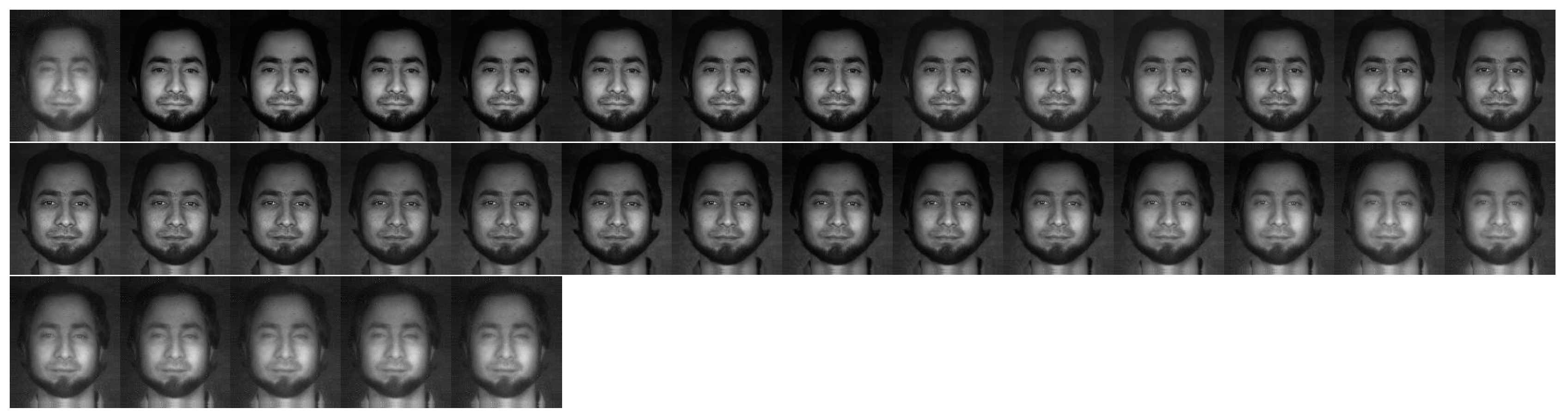
2.1. Hyper-Spectral Images

The spectral imaging method uses a generic imaging device to capture digital images over narrow fixed tens to hundreds of bands spanning the visible to infrared spectrum. Figure 2a illustrates a 3D data cube of the spectral imaging, which involves one dimensional spectral, and two dimensional spatial, information. Figure 2b illustrates the spectral reflectance properties of a point of a facial image. Its reflectance properties are affected by carotene, melanin and hemoglobin the three types of light-absorbing chemical compounds [14]. In addition to facial recognition, a spectral signature is widely used in liveliness studies by distinguishing a real human image from a synthetic mask or a mere photograph.

Apart from the above mentioned new opportunities, hyper-spectral imaging also poses a set of challenges, including a high spectral dimension, a low signal-to-noise ratio (SNR) and intra-person misalignment of bands. A high spectral dimension results in redundant information, which takes up large amounts of memory and is difficult to separate from useful information. Low-SNR information causes misjudgment of the results and affects experimental performance. The intra-person misalignment variations must be prohibited during the hyper-spectral imaging process. Most studies on the hyper-spectral image select discriminative and high-SNR information to improve experimental performance or simplify the calculation process [15,16]. Di et al. [15] selected a two subset feature center at the peak absorption bands (one consisting bands of 530 nm, 540 nm and 550 nm and another containing the bands of 570 nm, 580 nm and 590 nm). Li et al. [16] selected several bands with highly similar features to those of the first principle components (PCs) calculated by the principal component analysis (PCA).

2.2. Clustering Ensemble

The clustering ensemble algorithm has been developed as a more robust and stable [17] solution compared to individual clustering algorithms in the area of pattern recognition. Traditional individual clustering aims to classify unlabeled data into a homogeneous group, which lacks robust results. Additionally, many adaptations of classical clustering algorithms have been developed and the clustering ensemble algorithm has successfully attracted people’s attention [18,19,20]. In the past decade, literature on clustering ensemble has mainly been divided into three categories, including a paired similarity-based approach, a graph partitioning-based method approach and a median partition-based approach. The pair-wise similarity-based method constructs a co-association matrix as a similarity matrix to achieve the clustering [21]. The graph partitioning-based method regards the objects or clusters as graph nodes and builds graph links between them [22]. The median partition-based method visuals clustering as a point in high-dimensional space and finds its center through converting an optimization problem, which is to minimize the sum of distances (SOD) in the ensemble [23]. In this paper, clustering ensemble assembles the supervised and unsupervised process to achieve satisfactory segmentation performance.

3. Skin Feature Segmentation Scheme

In this section, the band selection algorithm and the algorithm for the generation of basic clustering are discussed in Section 3.1; the construction and re-labeling process for patches are proposed in Section 3.2; and the classification process is discussed in Section 3.3. Finally, the comparison methods are explained in Section 3.4.

3.1. Band Selection and Generation of Basic Clustering

To improve the performance of ensemble issues, N discriminative feature bands are selected as the input of k-means algorithm. The selected bands have highly similar features to those of the first PCs proposed by the Li et al. [16]. The first few PCs contain rich spatial information but it cannot ensure that the spectral signatures of interest are reserved. This method enhances the spatial features while emphasizing spectral signatures; thus, it is useful for the hyper-spectral image process. The similarity features are extracted from the widely used algorithm of Gray Level Co-occurrence Matrix (GLCM). Among 14 texture features of GLCM, the Inverse Difference Moment (IDM), contrast and entropy features are considered to be similarity criteria between the first PC and a single-band image to make sure the selected bands possess the greatest recognition ability. The contrast reflects the clarity of the image and the depth of the texture groove, whereas IDM reflects the homogeneity of the image texture and measures the local variation of image texture. Entropy measures the amount of information that an image has and indicates the degree of complexity of the image. The similarity criterion can be expressed as:

$${\ell }^l={\displaystyle \sum _{i=1}^3{{\displaystyle k}}_i}\left|\frac{{{\displaystyle PC}}_{{{\displaystyle F}}_i}-{{\displaystyle Band}}_{{{\displaystyle F}}_i}^l}{{{\displaystyle PC}}_{{{\displaystyle F}}_I}}\right|,l=1,2,3,\dots \mathrm{L}$$

(1)

where PC represents the first PC, ${{\displaystyle F}}_i$ represents the $i$th texture feature and ${{\displaystyle k}}_i$ represents the weight of the $i$th texture feature. The value of ${\ell }^l$ is metric of $l$th band. The smaller the value of metric ${\ell }^l$, the more the similarity between the first PC image and single bands is.

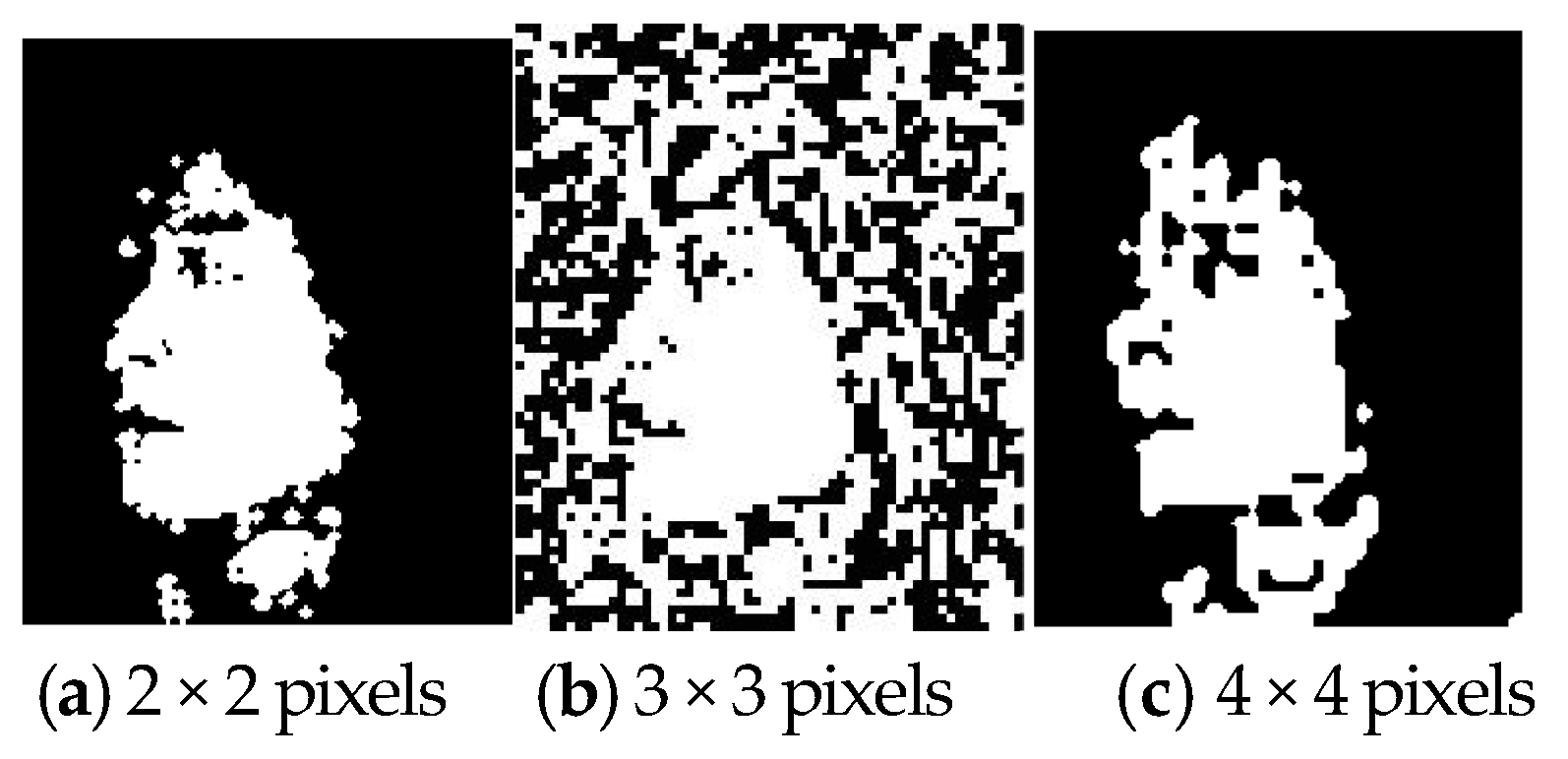
3.2. Construction and Re-Labeling of a Patch

In this subsection, due to a lack of a priori information, basic clustering is divided into a number of non-overlap neighborhoods as patch $\widehat{{\displaystyle X}}$, with a size arrangement of 2 × 2, 3 × 3, or 4 × 4 pixels. We depict a particular clustering distribution $k$th patch as a vector ${\gamma }_k$ and the vector value represents the number of clusters. The patch with the arrangement of 4 × 4 pixels is described as ${\gamma }_k$ = [a, b]. An example of binary clustering (the blue and orange cluster) can be seen in Figure 3, where ${\gamma }_a$ = [14, 2] and ${\gamma }_b$ = [2, 14], respectively. Figure 3a indicates that the patch has 14 pixels that belong to the blue cluster; and 2 pixels that belong to the red cluster. This can be analyzed based on Figure 3b. In this paper, clustering distribution comprises two clusters: skin or non-skin.

Hence, all of the basic clustering can be represented as patches ${\gamma }_k$, that is, the size of original basic clustering is 220 × 180; after being redefined with a size arrangement of 4 × 4 pixels and it becomes to 55 × 45 patches. Integrated with the selected basic clustering, patches with the samevalue remain as optional patches. According to the degree of the homogeneity rule, the optional patches with the highest homogeneity will be considered as the reliable patches called markers. Then the markers can be classified. In Figure 3, for example, as ${\gamma }_a$ = [14, 2] and ${\gamma }_b$ = [2, 14], we set $\widehat{{\displaystyle X_a}}$ to the blue cluster (${{\displaystyle L}}_a$ = 1) and set $\widehat{{\displaystyle X_b}}$ to the orange cluster (${{\displaystyle L}}_b$ = 2), which satisfy the rules 13 < a < 16 and 13 < b < 16. Specific situation rules depend on the size of the patch. Other unmarked patches need to be further classified. This method achieves reduced computational complexity and a faster execution speed.

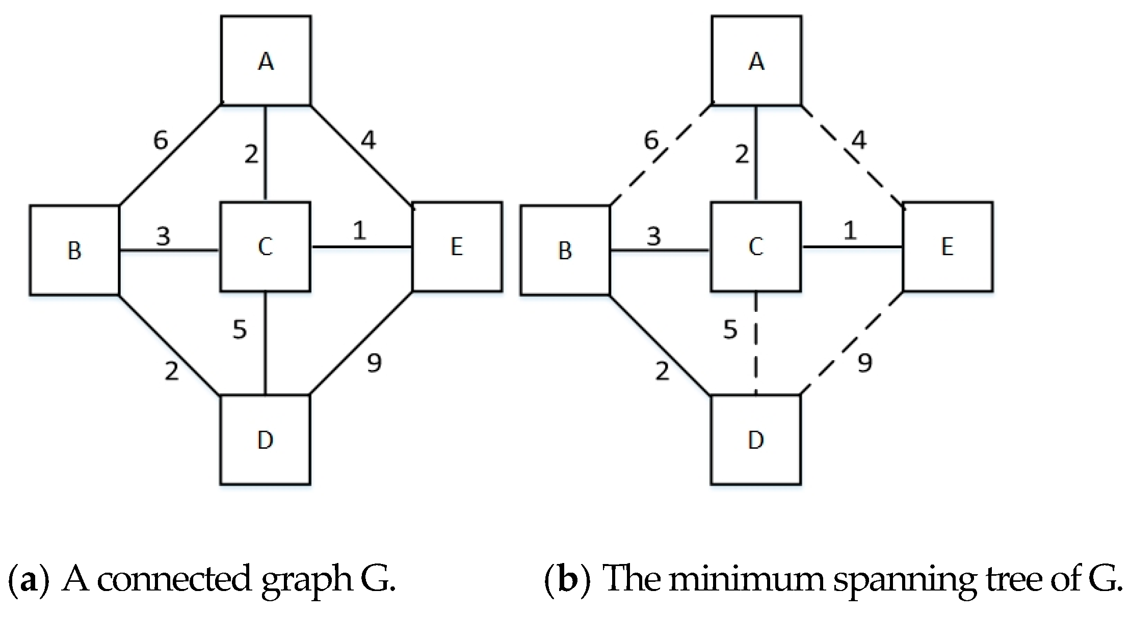
3.3. MSF for Classification

In this subsection, we group the adjacent image patches into series of MSF graphs with 3 × 3 blocks (see Figure 4) [24], that is, the size of image patches is 55 × 45; we need to calculate 18 × 15 graphs approximately. Thus, the spatial neighborhood information is fully considered by the calculated graphs.

The spanning forest graph is a weighted undirected and disconnected graph model that associates the weight or cost for each edge on the basis of the undirected graph. Additionally, the spanning forest graph is composed of a series of spanning tree graphs and is a weighted undirected and connected graph model.

Given a graph $G=\left(V,E,W\right)$, $V$ and $E$ are the sets of vertices (patch $\widehat{{\displaystyle X_k}}$) and edges (each edge ${{\displaystyle e}}_{ij}$ of this graph connects a couple of patches $i$ and $j$), respectively and W is a mapping of the set of edges E into ${{\displaystyle R}}^{+}$ (a weight ${{\displaystyle w}}_{ij}$ indicates the dissimilarity between two patches). In Figure 5a, there are a total of 5 vertices and they connected to each other with different weights. A Minimum spanning tree (MST) is rooted on one vertex (marker). The MST graph follows the principle that satisfies the minimum sum of edge weights, as expressed by the following equation:

$$T\in \underset{F\in ST}{{\displaystyle \arg \min }}\left\{{\displaystyle \sum _{{{\displaystyle e}}_{i,j\in {{\displaystyle E}}_T}}{{\displaystyle w}}_{i,j}}\right\}$$

(2)

where ST is a set of spanning trees of G. In Figure 5b, we generate a minimum spanning tree from graph of Figure 5a.

As mentioned above, the MSF is composed of a series of MSTs. Given a graph $G=\left(V,E,W\right)$, a MSF is rooted on a set of distinct vertices (a set of distinct markers), with each tree grown from one root vertex (marker). The principle of minimum sum of edge weights is expressed by the following equation:

$$F\in \underset{F\in SF}{{\displaystyle \arg \min }}\left\{{\displaystyle \sum _{{{\displaystyle e}}_{i,j\in {{\displaystyle E}}_F}}{{\displaystyle w}}_{i,j}}\right\}$$

(3)

where SF is a set of spanning forests of G rooted distinct vertices.

Then, uncertain patches classified into markers utilizing the spectral and spatial information generated by the MSF algorithm. The spectral similarity metric is based on mean information of patches, including Spectral Angle Mapper (SAM) and Spectral Information Divergence (SID). SID computes the probability behavior difference between the spectral signatures of two pixel vectors ${{\displaystyle x}}_i,{{\displaystyle x}}_j$:

$$SID({{\displaystyle x}}_i,{{\displaystyle x}}_j)=\left\{{\displaystyle \sum _{b=1}^B\{{{\displaystyle q}}_b({{\displaystyle x}}_i)\log \left[\frac{{{\displaystyle q}}_b({{\displaystyle x}}_i)}{{{\displaystyle q}}_b({{\displaystyle x}}_j)}\right]+}{{\displaystyle q}}_b({{\displaystyle x}}_j)\log \left[\frac{{{\displaystyle q}}_b({{\displaystyle x}}_j)}{{{\displaystyle q}}_b({{\displaystyle x}}_i)}\right]\right\}$$

(4)

SID is the degree of dissimilarity of two distributions, when ${{\displaystyle x}}_i,{{\displaystyle x}}_j$ has the same distribution and its value is 0. In this paper, ${{\displaystyle x}}_i$ and ${{\displaystyle x}}_j$ represent two different patches. The probability represents ${{\displaystyle q}}_b({{\displaystyle x}}_i)=\frac{\stackrel{-}{{{\displaystyle x}}_{lkb}}}{{\displaystyle \sum _{h=1}^B\stackrel{-}{{{\displaystyle x}}_{lkh}}}}$, where the mean spectral feature of the kth patch is derived from the following equation:

$${\overline{{\displaystyle x}}}_{lk}=\frac{{\displaystyle \sum _{l=1}^L{x}_{lk}}}{L},l=1,2\dots \mathrm{L}$$

(5)

where ${{\displaystyle x}}_{lk}={\left({{\displaystyle x}}_{1k},{{\displaystyle x}}_{2k},\dots {{\displaystyle x}}_{Lk}\right)}^T$ and $x_{lk}$ represents the $l$th pixel of the $k$th patch.

Actually, the above rules of finding the minimal sum of edge weights for graph can be resolved by a region-growing method. This means starting from a certain vertex as seed (marker) and gradually adding neighboring vertices (patches) according to the minimum weight certain criteria between two vertices of a graph. Prim’s algorithm can be used to achieve the MSF algorithm. An unlabeled patch $\hat{x}$ should be added to the seed every time, until all of the patches of the graph are classified. A prerequisite to be aware is that the graph should contain markers with different categories, as Figure 4a illustrates. Two classes of extra vertices ${{\displaystyle t}}_i$ ($i$ = 1, 2) are added to the graph linking the corresponding markers to form two categories of MST, as illustrated in Figure 4b. Each extra vertex is connected by the edge with a null weight to the markers. As illustrated in Figure 4c, markers are viewed as seeds; and unlabeled patches $\hat{x}$ are added to the tree to meet the criterion of minimum sum of the edge weights. While lacking markers are a common situation in a graph, we have to select markers manually. In this case, we select a marker within a graph that has the highest SID similarity to the nearest markers of this graph.

The whole algorithm can be indirectly listed as follows:

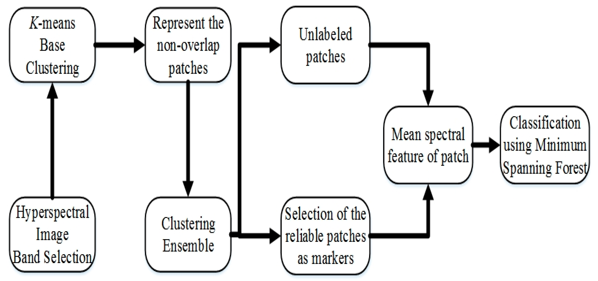
Step 1: Choose several discriminative basic clusters (see Section 3.2) as the input of the ensemble process.Step 2: The basic clustering is represented by non-overlap neighborhood patch $\hat{x}$ with 2 × 2 pixels. Depict it as a vector ${\gamma }_k$ and re-represent it by calculating the mean spectral characteristic ${\stackrel{-}{{\displaystyle x}}}_{lk}$.

Step 3: Integrate selected basic clustering, to obtain the optional patches. Then, select and re-label for reliable patches as markers, from the optional patches.

Step 4: Group the adjacent image patches into series of Minimum Spanning Forests with 3 × 3 blocks; and then assign the unlabeled patch ${\mathrm{x}}_{\mathrm{k}}$ to markers according to the SID similarity criterion.

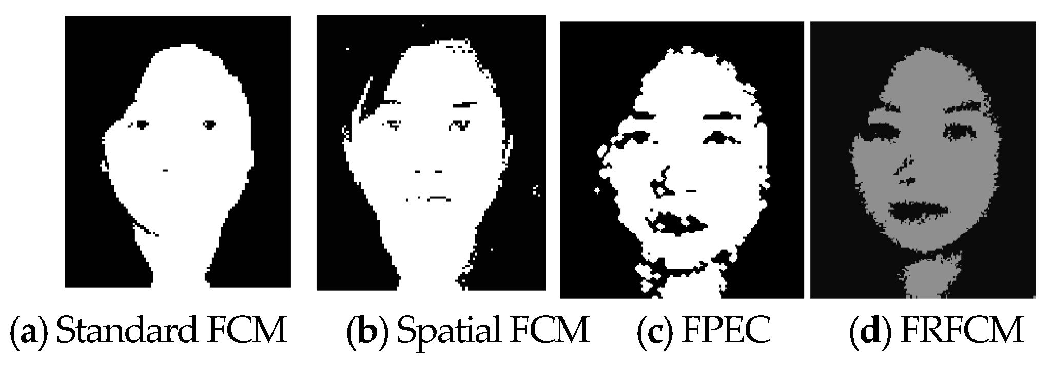
3.4. Comparison Algorithm

To evaluate the performance of the proposed algorithm, two algorithms are selected for comparison, including the standard fuzzy c-means (FCM) [25,26,27] and spatial FCM. Different from hard clustering k-means, FCM calculates the membership for each pixel to all clusters center. FCM is derived by iteratively minimizing a cost optimization function, that is, the weighted error of the sum of squares minimization inter-class. The function is defined as follows:

$$J={\displaystyle \sum _{\mathrm{j}=1}^N{\displaystyle \sum _{i=1}^c{{\displaystyle u}}_{ij}^m}}{\Vert {{\displaystyle x}}_j-{{\displaystyle v}}_i\Vert }^2$$

(6)

where $u_{ij}$ represents the membership of pixel $x_j$ (with N pixels) to the $i$th cluster and $v_i$ is the $i$th cluster center (with $c$ centroids). The parameter $m$ controls the fuzziness of the resulting partition and $m$ = 2 is used in the present study.

Neighboring pixels possess similar feature merit; thus, the probability that they belong to the same cluster is high. However, spatial features are not considered in the standard FCM. An improved method of FCM was proposed by Chuang et al. [28]; it incorporates spatial information into the membership function to improve the performance. A spatial function is defined as:

$$h_{ij}={\displaystyle \sum _{k\in NB({{\displaystyle x}}_j)}{{\displaystyle u}}_{ik}}$$

(7)

where ${{\displaystyle u}}_{ik}$ represents the membership of pixel ${{\displaystyle x}}_j$ belongs to the $k$th cluster and $NB({{\displaystyle x}}_j)$ represents the neighborhood pixels of a square window centered on pixel ${{\displaystyle x}}_j$. The improved membership function becomes:

$$u_{ij}{}^{\prime }=\frac{{{\displaystyle u}}_{ij}^p{{\displaystyle h}}_{ij}^q}{{\displaystyle \sum _{k=1}^c{{\displaystyle u}}_{ij}^p{{\displaystyle h}}_{ij}^q}}$$

(8)

where $p$ and $q$ are parameters that control the relative importance of both functions.

In this paper, SID is adapted to measure the distance between two distributions in the cost optimization function instead of using Euclidean Distance (ED). SID measures the differences in probability behavior between the spectral features of two pixel vectors based on the notion of divergence, which improves the clustering performance [29]. An improved FCM algorithm based on morphological reconstruction and membership filtering (FRFCM) is proposed by Tao et al. [30], that is significantly faster and more robust than FCM.

4. Experimental Results and Discussion

In this section, we conduct experiments on two public hyper-spectral facial image databases to evaluate the effectiveness of the proposed algorithm; as compared with standard FCM, spatial FCM and FRFCM algorithms.

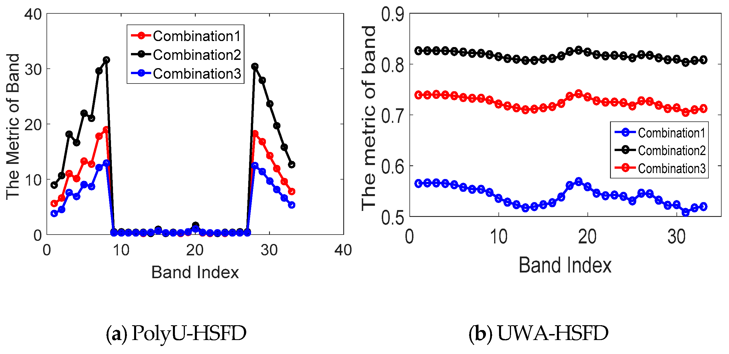
4.1. Band Selection Results

First, we adopt the mean value of four types of Gray Level Co-occurrence Matrixs (GLCMs) and the four different methods of scanning are horizontal, vertical, left and right diagonal. Then, we set different combination weights for contrast, entropy and IDM features, with 0.3, 0.5 and 0.2; 0.5, 0.2 and 0.3; and 0.2, 0.3 and 0.5, respectively. Based on Equation (1), we can observe the influence of the feature weight on the band selection result (see Figure 6 for one example).

Figure 6a illustrates the band selection result of the Hong Kong Polytechnic University Hyper-Spectral Face Database (PolyU-HSFD), in which the facial images of the 1, 2, 3, 4, 5, 6, 7, 28, 29, 30, 31, 32 and 33 bands have lower SNR in three different weight combinations. The Figure 6b from the University of Western Australia Hyper-Spectral Face Database (UWA–HSFD) indicates that the features on 25, 26, 27, 28, 29, 30, 31, 32 and 33 bands have the least effective information in three different weight combinations. This phenomenon is caused by the camera system. The sorting of the other bands indicates similarity in the first two weight combinations, so we site a greater weight for contrast to select the discriminative bands.

The above method has a perspective from mainly information and sorts the bands according to the amount of information relative to the first PC. There is a problem that the several bands contain similar local feature information. This is because the method does not consider the best categories’ separability between bands. After the sorting of information, we choose the best category’s separability bands according to the discrete metric. We select the several bands with less noise and high category separability as the input of the clustering ensemble. The results of the combination of the few bands indicate that the six bands (23, 22, 25, 13, 17 and 18) perform better for PolyU-HSFD; and the experiment that performs better includes the 18, 14, 16, 23, 28 and 12 bands for UWA-HSFD.

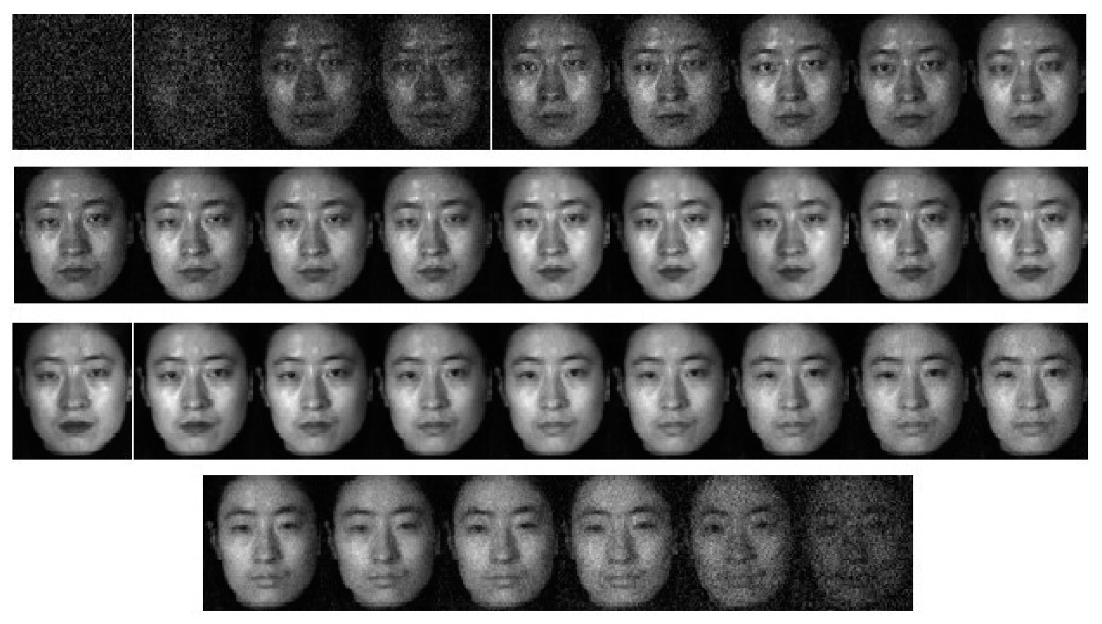
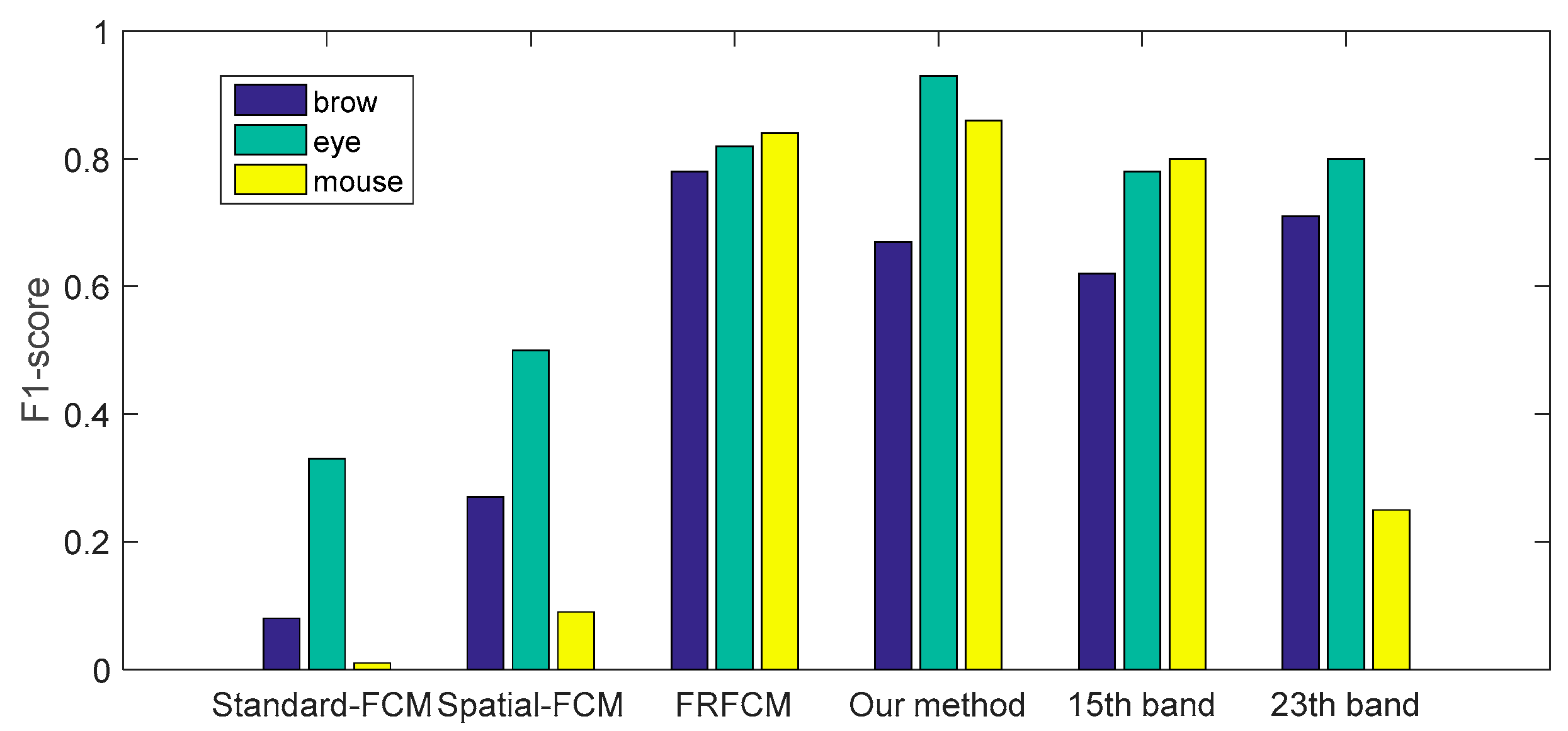
4.2. Skin Feature Segmentation of the PolyU Hyper-Spectral Face Database

The PolyU–HSFD, gathered by Di et al. [15] and acquired with the CRI’s VariSpec Liquid Crystal Tunable Filter (LCTF) and a Halogen Light system, consists of 25 data subjects of Asian descent (8 females and 17 males; 21–38 years old), with varying poses (frontal, right and left view of a subject) and time periods that include the hairstyle changes and skin condition diversification. Each data cube (see Figure 7 for one example) size is 220 × 180 × 33 pixels, with 33 bands covering the spectral range of 400–720 nm with a step size of 10 nm.

Figure 8a,b present basic clustering of facial images of front and left views, respectively. We can observe partial basic clustering with little effective feature information in Figure 8a, which is consistent with the band selection results of low-SNR bands. We can also find that specific local features stand out on distinct bands, while the bands with all of the local features are severely affected by noise (such as the last third basic clustering of Figure 8b). Hence, it is necessary to integrate discriminative basic clustering to get a robust result.

Next, we evaluate whether different sizes of a patch have an effect on the clustering ensemble’s results. It is not hard to find that we depict clustering distribution as patches and represent the patches’ feature information by calculating a mean spectral characteristic described in Section 3.2. The reason for this is that the patch is treated as the high-homogeneity neighborhood. Figure 9 illustrates the clustering ensemble results with a different patch size of the left view of the facial image of PolyU-HSFD. We can observe that the separation between features is poor with a large patch size of 4 × 4 pixels in Figure 9c. As the contour boundary of local features belongs to pixel mutation, the local feature boundary can be blurred if the neighborhood size is relatively large, especially if the two local features are close to each other, such as eyes and eyebrows, as illustrated in the Figure 9c. Instead, the clustering ensemble with a patch size of 2 × 2 pixels is more sensitive to contour boundaries of local features, as illustrated in the Figure 9a. As can be seen, a patch with a size of 3 × 3 pixels (Figure 9b) completely confuses the background and features.

The performance of the proposed algorithm with 2 × 2 and 4 × 4 pixels patch sizes are presented in

Table 1. Average comparison of different patch sizes of the proposed algorithm.

Block Size	Precision-Brow	Recall-Brow	F1-Score-Brow	Precision-Eye	Recall-Eye	F1-Score-Eye	Precision-Mouse	Recall-Mouse	F1-Mcore-Mouse
2 × 2	0.75	0.89	0.82	0.76	1.00	0.86	0.89	0.88	0.88
4 × 4	0.13	0.19	0.15	0.53	0.83	0.88	0.55	0.64	0.59

, in terms of precision, recall and F1-score. The recall reflects the proportion of the samples correctly classified as true positive samples (TP) to the positive samples that conclude true positive samples (TP) and the false negative samples (FN). It indicates the ability to identify positive samples. The recall can be expressed as:

$$\mathrm{R}=\frac{TP}{TP+FN}$$

(9)

The higher the recall is, the stronger the recognition ability of the positive samples is.

In addition, the precision reflects the proportion of the true positive samples (TP) to the test’s positive samples that conclude true positive samples (TP) and the false positive samples (FP). It indicates the ability to identify negative samples. The precision can be expressed as:

$$P=\frac{TP}{TP+FP}$$

(10)

The higher the precision is, the stronger the recognition ability of the negative samples is.

The F1-score is the combination of accuracy and the recall rate, which can be seen as the average effect. It reflects the robustness of the classification or segmentation model. The higher the F1-score is, the more robust the model is. The F1-score can be given according to:

$$F_{1-score}=\frac{2\cdot P\cdot R}{R+P}$$

(11)

In this database, we select three non-skin closed local features for assessment, for example, brows, eyes and a mouse. We can see that the 2 × 2 patch size achieves better performance, by improving the F1-score by 0.67%, −0.02% and 0.29% for local features. In general, the non-skin area features are more prominent in a 2 × 2 patch size, because the contour boundary is more obvious. Therefore, we choose the patch size of 2 × 2 pixels for the proposed algorithm in all the following experiments.

Finally, the performance of the proposed algorithm on PolyU-HSFD is compared with the previously mentioned standard FCM, spatial FCM, FRFCM and basic clustering. In Figure 10a (front facial image), the standard FCM clustering loses numerous features, because spectral reflectance of the face is not a reliable biometric, as spectral reflectance will change slightly due to the external environment [31]. Figure 10b illustrates spatial FCM clustering that performs better than the standard FCM algorithm as it makes full use of the spatial and spectral information, as expressed by Equation (7). This is achieved by adding the spatial function to the membership function ${\mathrm{u}}_{\mathrm{i}\mathrm{j}}^{\mathrm{m}}$ as expressed by Equation (8). Figure 10c illustrates the performance of the proposed algorithm, in which almost all local features are obvious. Figure 10d also indicates a good result using a fast and robust FCM (FRFCM) algorithm.

Table 2. Average effect comparison of different model methods for PolyU-HSFD.

Method	Precision-Brow	Recall-Brow	Precision-Eye	Recall-Eye	Precision-Mouse	Recall-Mouse
Standard-FCM	0.92	0.04	0.97	0.2.0	0	0
spatial-FCM	0.62	0.17	0.85	0.35	0.82	0.05
FRFCM	0.65	0.96	0.79	0.84	0.89	0.79
Our method	0.67	0.67	0.96	0.91	0.93	0.80
15th band	0.59	0.66	0.80	0.77	1.00	0.66
23rd band	0.67	0.86	0.82	0.78	1.00	0.14

and Figure 11 summarize the results. Compared with spatial FCM, which makes full use of all spectral and spatial information, our method performs better and the F1-score rate improved by 0.11%, 0.43% and 0.77% for local features. Compared with the better basic clustering of the 23rd band and FRFCM, the F1-score rate is improved by −0.04%, 0.13% and 0.61% as well as −0.11%, 0.11 and 0.02% for local features. The non-skin area features are more prominent in our proposed method.

However, the feature characteristics of the right wing of the nose are not obvious. These features are highlighted in the low SNR bands, which are not selected into the ensemble process. Hence, basic clustering has a significant impact on ensemble results.

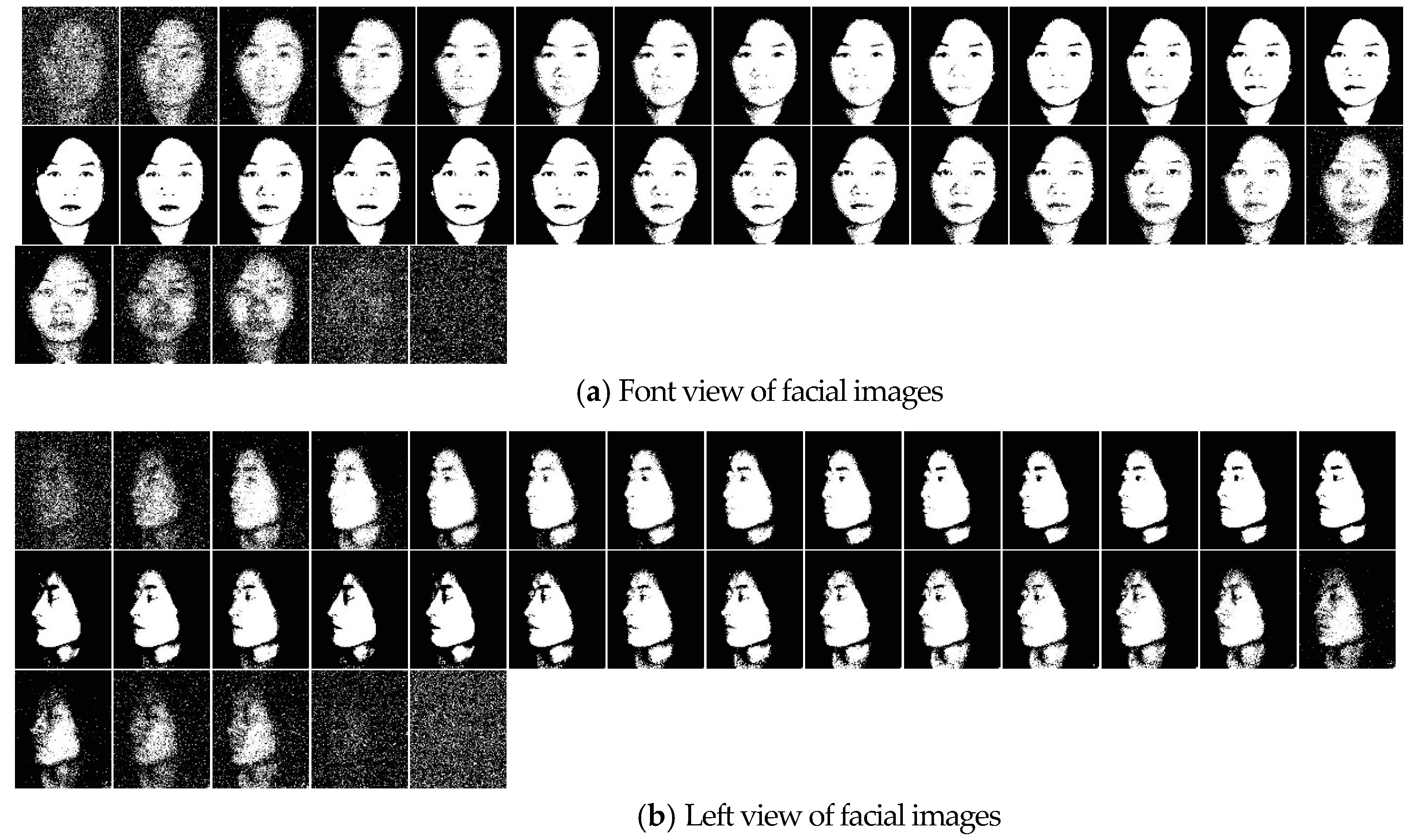
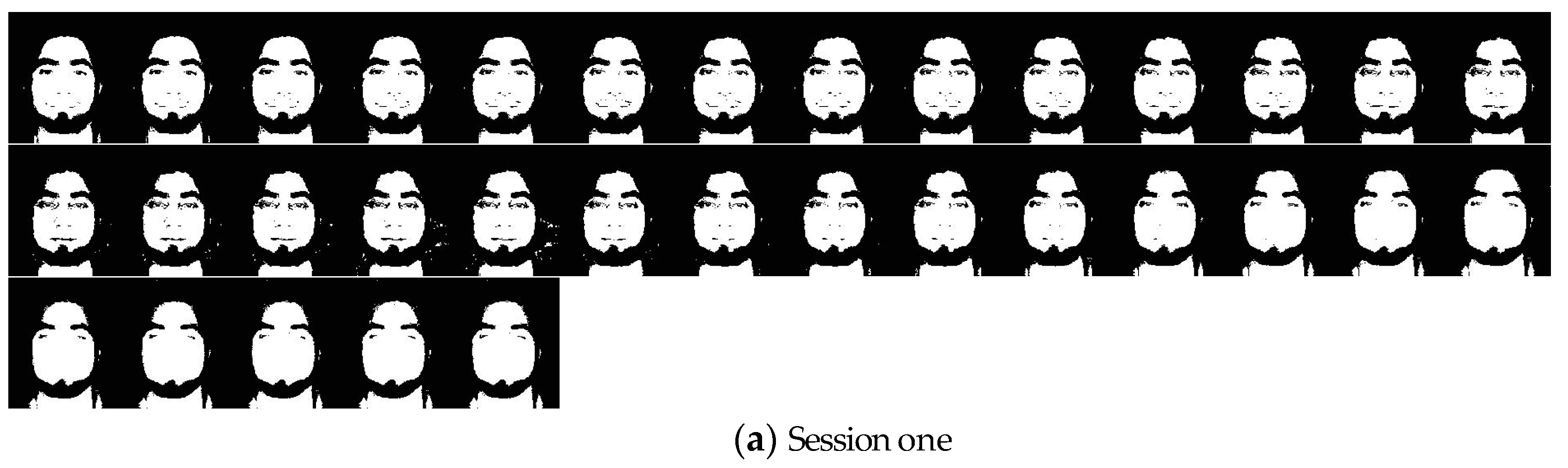
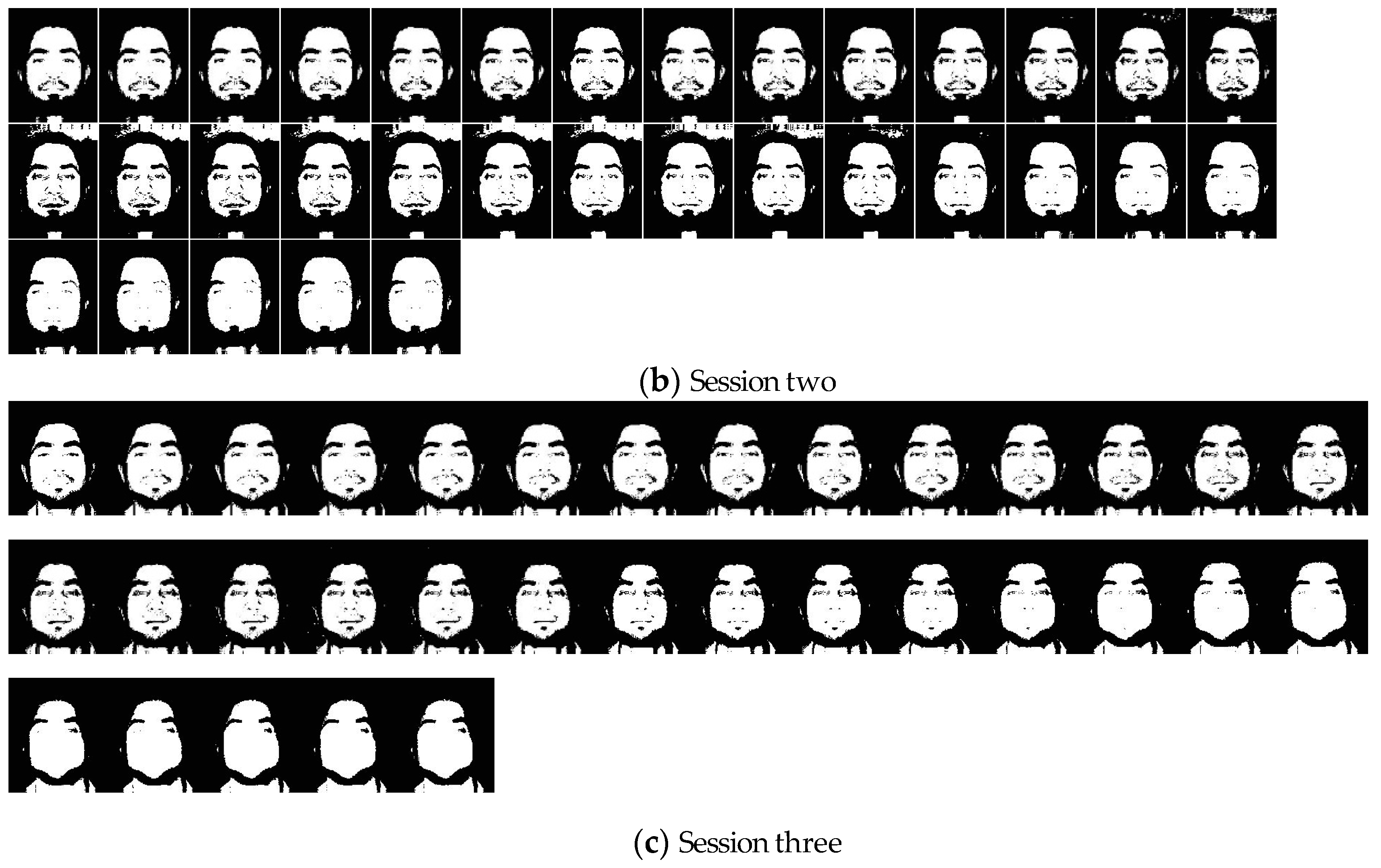
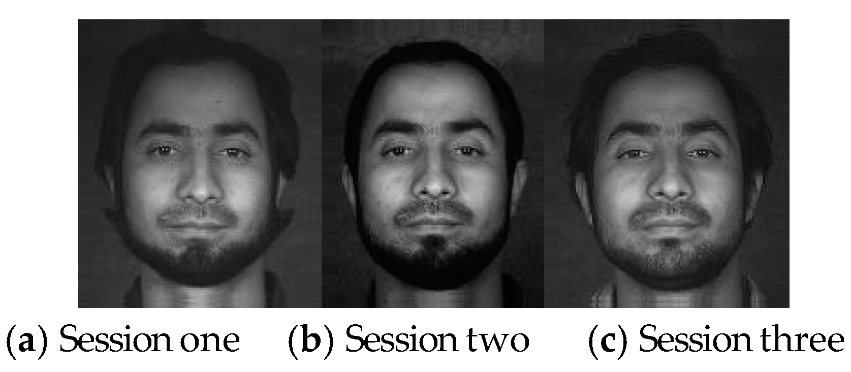
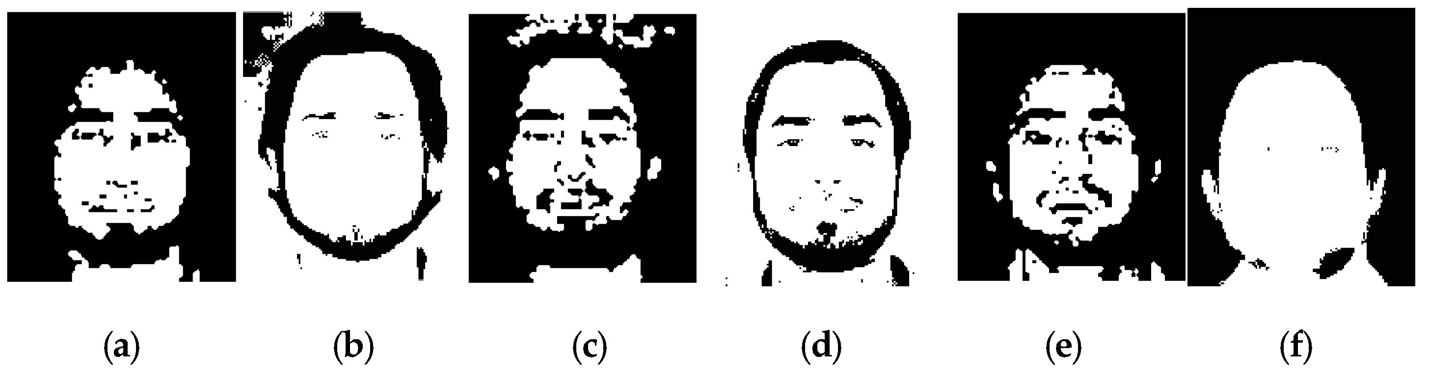
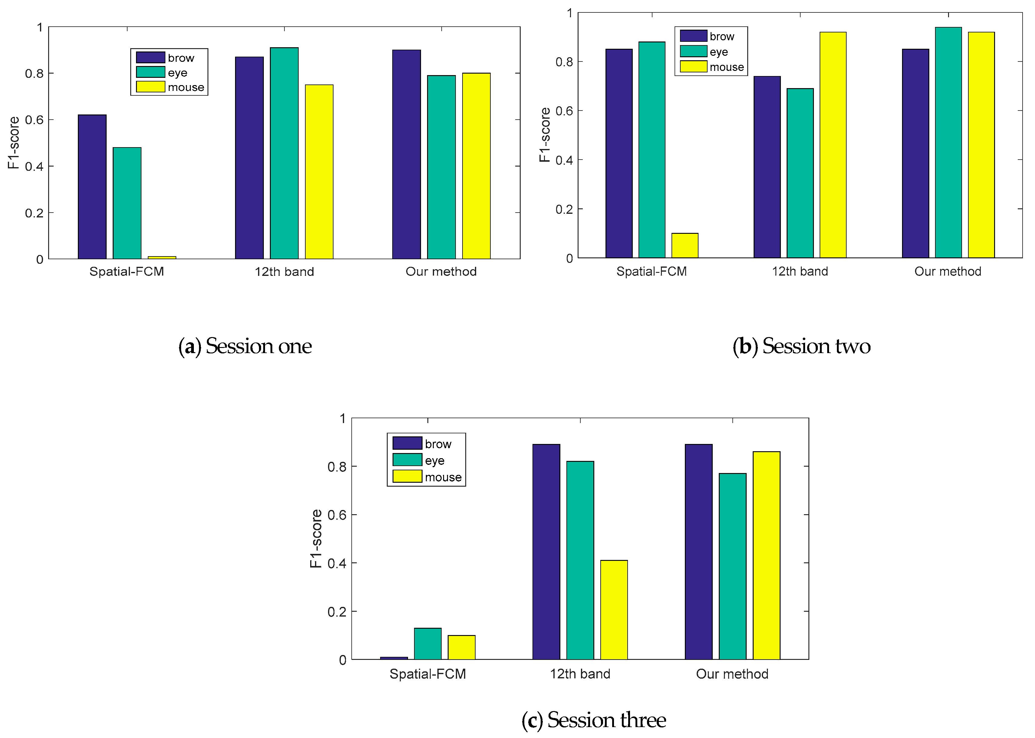
4.3. Skin Feature Segmentation of the UWA Hyper-Spectral Face Database

UWA-HSFD is acquired with the CRI’s VariSpec Liquid Crystal Tuneable Filter (LCTF) and integrated with a photon focus camera. UWA-HSFD consists of 79 data subjects in the frontal view taken over 1–4 sessions (see Figure 12 for one example) [32,33]. Each data cube of a hyper-spectral facial image contains 33 bands covering the visible spectral range from 400 to 720 nm with a 10 nm step. The SNR in this database is relatively lower because Uzair et al. [31] used a novel algorithm that automatically adjusted the camera exposure time based on the filter’s transmittance, illumination intensity and CCD sensitivity for each frequency band. Most subjects had slight head movements and eye blinking during image collection process, therefore, there was alignment errors between individual bands.

In our experiment, each subject in the databases was cropped to a different size according to his/her position from the background. We selected data cubes with little inter-misalignments in three sessions. Figure 13 illustrates basic clustering with three sessions of the same subject. Once again, this proves that local features are highlighted on distinct bands. We selected three local features for assessment: beard, eyes and brows, which highlight the biological characteristics of the beard. According to the band selection results, the bands highlighting different features with less noise are selected as the input of the clustering ensemble.

In addition, we can observe that the basic clustering of session one had a poor performance of nose characteristics. In session two, several bands in the middle have some noise in the front of the images. That may be due to imaging photographic light.

The performance for the proposed algorithm in Figure 15a,c,e is compared with spatial FCM in Figure 15b,d,f and the basic clustering, respectively. We can observe that the local features nose and mouth are not recognized for session one, as illustrated in Figure 15b and the recognition is not complete and clear for session two, as shown in Figure 15d. The most unsatisfactory result has little useful information for session three, as illustrated in Figure 15f. Relatively speaking, local features are clear and complete in the clustering ensemble.

Table 3. Average effect comparison of different model methods for UWA-HSFD of session one.

Method	Precision-Brow	Recall-Brow	Precision-Eye	Recall-Eye	Precision-Beard	Recall-Beard
spatial-FCM	1.00	0.45	1.00	0.32	0	0
12th band	0.77	1.00	0.95	0.87	0.94	0.62
Our-method	0.93	0.88	0.76	0.82	0.89	0.72

,

Table 4. Average effect comparison of different model methods for UWA-HSFD of session two.

Method	Precision-Brow	Recall-Brow	Precision-Eye	Recall-Eye	Precision-Beard	Recall-Beard
spatial-FCM	0.85	0.86	0.93	0.84	1.00	0.05
12th band	0.58	1	0. 64	0.75	1.00	0.84
Our-method	0.83	0.88	1.00	0.88	1.00	0.84

and

Table 5. Average effect comparison of different model methods for UWA-HSFD of session three.

Method	Precision-Brow	Recall-Brow	Precision-Eye	Recall-Eye	Precision-Beard	Recall-Beard
Spatial-FCM	0	0	1.00	0.07	0	0
12th band	0.83	0.96	1.00	0.70	0.83	0.27
Our-method	0.85	0.93	0.83	0.71	1.00	0.77

and Figure 16. illustrate the performance evaluations of three local features (brows, eye and beard) for three sessions. Compared with the better basic clustering of the 12th band, the F1-score rate improved by 0.03%, −0.12% and 0.05% for local features in session one; 0.11%, 0.25% and 0% for local features in session two; and 0%, −0.05% and 0.45% for local features in session three. Compared with the spatial FCM, the F1-score rate improved by 0.28%, 0.31% and 0.80% for local features in session one; 0%, 0.06% and 0.82% for local features in session two; and 0.89%, 0.64% and 0.86% for local features in session 3. Totally, the proposed algorithm is superior to other two algorithms.

However, as illustrated in Figure 15a, we notice that the nose feature is unsatisfactory in the clustering ensemble of session one, caused by basic clustering as illustrated in Figure 13a. There is noise interference in the front of clustering ensemble that can be found in Figure 15c. In this case, we use the location information for feature extraction to avoid being affected by noise interference in the front of facial image. Therefore, basic clustering plays an essential role in the ensemble process.

5. Conclusions

In this article, we present an effective skin feature-segmentation method for a hyper-spectral facial image. Instead of segmentation of an unlabeled point on a pixel-by-pixel basis, we make full use of spatial structure information on the neighborhood and spectral information for the MSF classification algorithm process. We evaluate the performance of the proposed method on two databases with uncontrolled conditions. Experimental results have proven that the proposed algorithm outperforms the other algorithms. Our algorithm can also perform better for skin segmentation of a facial image in complex environments and in classification for a remote sensing image.

As mentioned in our experiments, the ensemble results are significantly influenced by the performance of basic clustering. In a more complex background environment, other clustering methods should be considered to improve the local feature performance in basic clustering, just like the different color space in RGB images, in future works. Another phenomenon in the experiment is that a marker around a patch affects the clustering ensemble results. It is time-consuming to repeat the experiment to select the best performance markers. Hence, designing the selection of a reliable marker around the patch is a direction of our future work. It is worth mentioning that, sub-sampling image needed some operators to fill holes and remove small protrusion.

References

1. Ross, A.; Jain, A.K.; Qian, J.Z. Information Fusion in Biometrics. In Proceedings of the International Conference on Audio- and Video-Based Biometric Person Authentication, Halmstad, Sweden, 6–8 June 2001. [Google Scholar]
2. Al-Tairi, Z.H.; Rahmat, R.W.; Saripan, M.I.; Sulaiman, P.S. Skin segmentation using YUV and RGB color spaces. J. Inf. Process. Syst. 2014, 10, 283–299. [Google Scholar] [CrossRef]
3. Chelali, F.Z.; Cherabit, N.; Djeradi, A. Face recognition system using skin detection in RGB and YCbCr color space. In Proceedings of the Web Applications and Networking, Sousse, Tunisia, 21–23 March 2015. [Google Scholar]
4. Kawulok, M. Fast propagation-based skin regions segmentation in color images. In Proceedings of the IEEE International Conference and Workshops on Automatic Face and Gesture Recognition, Shanghai, China, 22–26 April 2013. [Google Scholar]
5. Chen, W.; Wang, K.; Jiang, H.; Li, M. Skin color modeling for face detection and segmentation: A review and a new approach. Multimed. Tools Appl. 2016, 75, 839–962. [Google Scholar] [CrossRef]
6. Tan, W.R.; Chan, C.S.; Yogarajah, P.; Condell, J. A Fusion Approach for Efficient Human Skin Detection. IEEE Trans. Ind. Inform. 2012, 8, 138–147. [Google Scholar] [CrossRef] [Green Version]
7. Xu, T.; Wang, Y.; Zhang, Z. Pixel-wise skin colour detection based on flexible neural tree. IET Image Process. 2013, 7, 751–761. [Google Scholar] [CrossRef]
8. Naji, S.A.; Zainuddin, R.; Jalab, H.A. Skin segmentation based on multi pixel color clustering models. Digit. Signal Process. 2012, 22, 933–940. [Google Scholar] [CrossRef]
9. Chai, D.; Ngan, K.N. Face segmentation using skin-color map in videophone applications. IEEE Trans. Circuits Syst. Video Technol. 1999, 9, 551–564. [Google Scholar] [CrossRef]
10. Marzec, M.; Koprowski, R.; Wróbel, Z. Methods of face localization in thermograms. Biocybern. Biomed. Eng. 2015, 35, 138–146. [Google Scholar] [CrossRef]
11. Filipe, S.; Alexandre, L.A. Thermal Infrared Face Segmentation: A New Pose Invariant Method; Springer: Berlin/Heidelberg, Germany, 2013; pp. 632–639. [Google Scholar]
12. Filipe, S.; Alexandre, L.A. Algorithms for invariant long-wave infrared face segmentation: Evaluation and comparison. Pattern Anal. Appl. 2014, 17, 823–837. [Google Scholar] [CrossRef]
13. Glowacz, A.; Glowacz, Z. Diagnosis of the three-phase induction motor using thermal imaging. Infrared Phys. Technol. 2016, 81, 7–16. [Google Scholar] [CrossRef]
14. Zonios, G.; Bykowski, J.; Kollias, N. Skin melanin, hemoglobin, and light scattering properties can be quantitatively assessed in vivo using diffuse reflectance spectroscopy. J. Investig. Dermatol. 2001, 117, 1452–1457. [Google Scholar] [CrossRef] [PubMed]
15. Di, W.; Zhang, L.; Zhang, D.; Pan, Q. Studies on Hyperspectral Face Recognition in Visible Spectrum with Feature Band Selection. IEEE Trans. Syst. Man Cybern. Part A Syst. Hum. 2010, 40, 1354–1361. [Google Scholar] [CrossRef]
16. Li, Y.; Xie, W.; Li, H. Hyperspectral image reconstruction by deep convolutional neural network for classification. Pattern Recognit. 2016, 63, 371–383. [Google Scholar] [CrossRef]
17. Huang, D.; Lai, J.; Wang, C.D. Ensemble clustering using factor graph. Pattern Recognit. 2016, 50, 131–142. [Google Scholar] [CrossRef]
18. Zhao, F.; Jiao, L.; Liu, H.; Gao, X.; Gong, M. Spectral clustering with eigenvector selection based on entropy ranking. Neurocomputing 2010, 73, 1704–1717. [Google Scholar] [CrossRef]
19. Bin, Z.; Chijie, Z.H.; Jun, H. Ensemble Clustering Algorithm Combined With Dimension Reduction Techniques for Power Load Profiles. Proc. CSEE 2015, 35, 3741–3749. [Google Scholar]
20. He, M.; Yang, Y.; Wang, S. NMF-Based Clustering Ensemble Algorithm. Comput. Sci. 2017, 44, 58–61. (In Chinese) [Google Scholar]
21. Yi, J.; Yang, T.; Jin, R.; Jain, A.K.; Mahdavi, M. Robust Ensemble Clustering by Matrix Completion. In Proceedings of the IEEE International Conference on Data Mining, Brussels, Belgium, 10–13 December 2012. [Google Scholar]
22. Fern, X.Z.; Brodley, C.E. Solving cluster ensemble problems by bipartite graph partitioning. In Proceedings of the International Conference on Machine Learning, Banff, AB, Canada, 4–8 July 2004. [Google Scholar]
23. Franek, L.; Jiang, X. Ensemble clustering by means of clustering embedding in vector spaces. Pattern Recognit. 2014, 47, 833–842. [Google Scholar] [CrossRef]
24. Tarabalka, Y.; Chanussot, J.; Benediktsson, J.A. Segmentation and classification of hyperspectral images using minimum spanning forest grown from automatically selected markers. IEEE Trans. Syst. Man Cybern. B Cybern. 2010, 40, 1267–1279. [Google Scholar] [CrossRef] [PubMed]
25. Bezdek, J.C.; Ehrlich, R.; Full, W. FCM: The fuzzy c-means clustering algorithm. Comput. Geosci. 1984, 10, 191–203. [Google Scholar] [CrossRef]
26. Shokouhi, S.B.; Fooladivanda, A.; Ahmadinejad, N. Computer-aided detection of breast lesions in DCE-MRI using region growing based on fuzzy C-means clustering and vesselness filter. EURASIP J. Adv. Signal Process. 2017, 2017, 39. [Google Scholar] [CrossRef] [Green Version]
27. Shi, A.; Gao, G.; Shen, S. Change detection of bitemporal multispectral images based on FCM and D-S theory. EURASIP J. Adv. Signal Process. 2016, 2016, 96. [Google Scholar] [CrossRef]
28. Chuang, K.S.; Tzeng, H.L.; Chen, S.; Wu, J.; Chen, T.J. Fuzzy c-means clustering with spatial information for image segmentation. In Proceedings of the International Conference on Electrical Engineering, Lahore, Pakistan, 9–11 April 2009. [Google Scholar]
29. Chang, C.I. An information-theoretic approach to spectral variability, similarity, and discrimination for hyperspectral image analysis. IEEE Trans. Inf. Theory 2000, 46, 1927–1932. [Google Scholar] [CrossRef]
30. Lei, T.; Jia, X.; Zhang, Y.; He, L.; Meng, H.; Nandi, A.K. Significantly Fast and Robust Fuzzy C-Means Clustering Algorithm Based on Morphological Reconstruction and Membership Filtering. IEEE Trans. Fuzzy Syst. 2018, 26, 3027–3041. [Google Scholar] [CrossRef]
31. Uzair, M.; Mahmood, A.; Shafait, F.; Nansen, C.; Mian, A. Is spectral reflectance of the face a reliable biometric? Opt. Express 2015, 23, 15160–15173. [Google Scholar] [CrossRef] [PubMed]
32. Uzair, M.; Mahmood, A.; Mian, A. Hyperspectral Face Recognition with Spatiospectral Information Fusion and PLS Regression. IEEE Trans. Image Process. 2015, 24, 1127–1137. [Google Scholar] [CrossRef] [PubMed]
33. Uzair, M.; Mahmood, A.; Mian, A. Hyperspectral Face Recognition using 3D-DCT and Partial Least Squares. BMVC 2013. [Google Scholar] [CrossRef]
Figure 1. Flow chart of the proposed algorithm.
Information 09 00261 g001
Figure 2. An example of a hyper-spectral facial image cube (a); and normalized spectrum of face local region (b).
Information 09 00261 g002
Figure 3. Examples of two different distributions of a patch with 4 × 4 pixels.
Information 09 00261 g003
Figure 4. An example of the construction of an MSF rooted on markers proposed by Tarabalka et al. [25]. (a) Original image graphs G. 1 and 2 represent the labeled patches (markers); unlabeled patches are denoted by “0”. (b) Addition vertices t 1 , t 2 to the graph G. (c) The MSF with two MSTs of graph G.
Information 09 00261 g004
Figure 5. An example of the process of a minimum spanning tree.
Information 09 00261 g005
Figure 6. Band selection metric of two databases.
Information 09 00261 g006
Figure 7. A hyper-spectral facial image from the PolyU-HSFD.
Information 09 00261 g007
Figure 8. Results of single band clustering with different views from the PolyU-HSFD.
Information 09 00261 g008
Figure 9. Ensemble clustering with different patch sizes.
Information 09 00261 g009
Figure 10. Ensemble clustering with different methods.
Information 09 00261 g010
Figure 11. Robust comparison of different model methods for PolyU-HSF.
Information 09 00261 g011
Figure 12. Hyperspectral facial image from the UWA-HSFD.
Information 09 00261 g012
Figure 13. Single band clustering of three different periods correspond to Figure 14 of UWA-HSFD.
Information 09 00261 g013aInformation 09 00261 g013b
Figure 14. The 16th band image of the same person in three different sessions from the UWA-HSFD.
Information 09 00261 g014
Figure 15. FPEC and spatial FCM clustering for three sessions (a,c,e) are FPEC clustering and (b,d,f) are the spatial FCM clustering, which corresponds to Figure 14.
Information 09 00261 g015
Figure 16. Robust comparison of different model methods for UWA-HSFD.
Information 09 00261 g016