Detecting Anomalous Trajectories Using the Dempster-Shafer Evidence Theory Considering Trajectory Features from Taxi GNSS Data

Abstract

In road networks, an ‘optimal’ trajectory is a geometrically optimal drive from the source point to the destination point. In reality, the driver’s driving experience or road traffic conditions will lead to differences between the ‘actual’ trajectory and the ‘optimal’ trajectory. When the differences are excessive, these trajectories are considered as anomalous trajectories. In addition, these differences can be observed in various trajectory features, such as velocity, distance, turns, and intersections. In this paper, our aim is to fuse these trajectory features and to quantitatively describe this difference to infer anomalous trajectories. The Dempster-Shafer (D-S) evidence theory is a theory and method that uses different features as evidence to infer uncertainty. The theory does not require prior knowledge or conditional probabilities. Therefore, we propose an automatic, anomalous trajectory inference method based on the D-S evidence theory that considers driving behavior and road network constraints. To achieve this objective, we first obtain all of the ‘actual’ trajectories of drivers for different source-destination pairs in taxi Global Navigation Satellite System (GNSS) trajectories. Second, we define and extract five trajectory features: route selection ($RS$), intersection rate ($IR$), heading change rate $\left(\mathrm{HCR}\right)$, slow point rate ($\mathrm{SPR}$), and velocity change rate $\left(\mathrm{VCR}\right)$. Then, different features of each trajectory are combined as evidence according to Dempster’s combinational rule. The precise probability interval of each trajectory is calculated based on the D-S evidence theory. Finally, we obtain the anomalous possibility of all real trajectories and infer anomalous trajectories whose trajectory features are significantly different from normal ones. The experimental results show that the proposed method can infer anomalous trajectories effectively and that it can be used to monitor driver behavior automatically and to discover adverse urban traffic events.

1. Introduction

1.1. Purpose and Significance

As a part of urban public transport, taxis are equipped with GNSS navigation equipment [1] and can be used as flow monitors of urban traffic to generate massive GNSS trajectory data over time. Such data can well reflect people’s daily travel behavior and urban traffic conditions [2]. Meanwhile, they are associated with irrational phenomenon such as traffic congestion, the refusal to take passengers, taxi fraud, and detours, etc. [3]. These phenomena can cause anomalous trajectories in the trajectory data. Therefore, it is necessary to discover such phenomena using anomalous trajectory detection research.

Anomalous detection has many important applications. In the field of fraudulent actions, human fraudulent behavior is detected automatically based on trajectories extracted from videos [4,5,6]. In the field of traffic safety, traffic events are detected by using video detection data in urban traffic automatically, and the relationship between events and conflict is analyzed [7,8,9]. For GNSS trajectory data, they have two areas of application: one is to discover anomalous traffic [10,11], and the other is to infer anomalous trajectories [12,13,14,15]. Our research focuses on the detection of anomalous trajectories. The research plays an important role in the monitoring of driver behavior and activity safety, the improvement of taxi service levels, and urban traffic conditions.

In recent years, anomalous trajectory detection has included the distance-based method [16,17], the clustering-based method [12,18,19], the classification-based method [20,21], and the grid-based method [13,14,15]. The distance-based method divides the whole trajectory into sub-trajectories that include certain trajectory points and calculates the Hausdorff distance between sub-trajectories. This method involves high computational intensity and difficulty in addressing GNSS trajectories with high sparsity [22]. The clustering-based method calculates the similarity of trajectories and selects an appropriate clustering method. The similarity of the trajectory is mostly described by considering the distance between the trajectory points or the trajectory segments. Commonly used distances include, for example, the Euclidean distance, dynamic time warping (DTW), and edit distance (ED) [12]. The trajectories are unevenly distributed, and it is difficult to exhibit aggregation. The research data are almost all trajectories from same source-destination pairs [12]. The classification-based method builds a classification model based on trajectory features and requires more sample data for learning and training. In practical applications, it is difficult for researchers to find training data covering all anomalous labels. The above studies use simulated data or video surveillance data [21]. The grid-based method expresses a trajectory in a dividing grid, which can reduce the computational requirements and accelerate the speed and accuracy of detection. The size of the grid determines the accuracy of the trajectory distance. Some scholars use the adaptive window size to solve this problem [14].

Overall, these studies consider the interaction between trajectories. Relevant methods are aimed at finding patterns based on the similarity of trajectories, including velocity similarity, distance similarity, and spatial-time similarity. Trajectories deviating from these patterns are defined as anomalies. However, when the amount of data becomes large, normal patterns can be covered by other trajectory data, and anomalous trajectories might form new patterns, which results in inaccurate results or limitations on processing data. Therefore, some researchers consider a single individual trajectory and assume that the trajectories do not affect each other. The related research is less and aims to judge whether the trajectory is anomalous by calculating the basic or high-level features of the trajectory. Some basic features of the single trajectory include speed, position, and time [20,23]. They also define some high-level features such as turns, detours, and route repetition [24]. The relevant methods mainly include the classification-method [20,23], and the uncertain reasoning methods, etc. [24,25,26]. The classification-based method uses the features of the sample trajectories to construct a classifier that classifies trajectories. This method requires the participation of a large number of samples, and the quality of the training samples affects the result. The uncertain reasoning method fuses these features of the trajectory to obtain the anomalous probability of the trajectory.

Our research focuses on the anomaly judgment of the individual trajectory. Due to privacy protection, data storage and other issues, many taxi trajectory data do not record driver’s personal information and passenger feedback information. The data lack a description of the trajectory anomaly. Some uncertain reasoning methods containing fuzzy inference or the Bayesian network method require a large amount of sample data with known result labels. For taxi trajectory data, a large amount of tagged training data is more difficult to obtain. The Dempster-Shafer (D-S) theory is a mathematical theory of evidence based on belief functions and plausible reasoning [27]. The definite advantage of the D-S evidence theory is that it does not require prior knowledge or conditional probabilities and is suitable for classifying data with unknown result labels. Furthermore, it can provide information concerning uncertainty about analyzed problems. The evidence in the D-S theory refers to the probability of support for all questions to be identified.

1.2. Anomalous Trajectory Definition

In order to achieve our purpose, we need to redefine the anomalous trajectory. ‘Anomalous trajectories’ can be very diversely defined in different applications [24]. For example, some studies focus on the behavior of driver fraud and define trajectories of detours or loops as anomalous trajectories [25,28]. Some researchers consider the similarity of trajectories to cluster trajectories, and those clusters with smaller numbers or isolated trajectories are defined as anomalous trajectories [12,13]. Some scholars define normal behavior as driving from the source point to the destination point through the optimal route, and anomalous trajectories are defined as those trajectories in which various anomalous behaviors can occur, such as taking a wrong turn, getting lost, and turn restrictions [24]. Previous studies are mostly concerned with one aspect of trajectory anomalies. If the purpose of the study is to find the maximum or minimum value of the trajectory distance, time, velocity, etc., it can be achieved using simple statistics. Our work is not limited to this and is to detect trajectories with obvious anomalous behavior. In fact, anomalous trajectories are generated for various reasons, which include the subjective behavior of drivers or passengers, and the complex traffic conditions of the road network. We need to analyze the causes of the anomalous trajectory as much as possible and define appropriate trajectory features that reflect anomalous behaviors.

Therefore, to infer the anomalous trajectory, we introduce the ‘optimal’ trajectory as the normality of the trajectory. An ‘optimal’ trajectory is defined as a geometrically optimal driving of road networks from the source point to the destination point without knowing the driver’s driving experience or the road traffic conditions. As shown in Figure 1a, the black dotted line is an ‘optimal’ trajectory. For the ‘optimal’ trajectory, the velocity of each sampling point is the same, and the trajectory does not have frequent turns, detours, or route repetitions. In contrast to the ‘optimal’ trajectory, the driver will choose different road sections according to their driving experience or passenger requirements. Various special traffic situations can occur on the road networks, such as traffic congestion, traffic accidents, and traffic restrictions. This will lead to a difference between the ‘actual’ trajectory and the ‘optimal’ trajectory. As shown in Figure 1b, the black solid line is the ‘actual’ trajectory, the velocity of each sample point is different, and the distance between the sample points is different. When the difference is excessive, these trajectories are defined as anomalous trajectories.

The difference between the ‘actual’ trajectory and the ‘optimal’ trajectory needs to be quantified as a criterion for judging whether a trajectory is anomalous. The trajectory features can be used for the observations of the ‘actual’ trajectory, as caused by the corresponding driving experience and special events. For D-S evidence theory, the question is whether the trajectory is anomalous or normal, and the probability that each feature supports the problem constitutes evidence. We view the trajectory features as different evidence of the anomalous trajectory observation and use the D-S theory to fuse the evidence. The optimal trajectory, usually in urban areas, is computed with reference to so-called generalized costs [29]. When the cost of consideration is different, such as time, distance, or price, the optimal route is not the same. Due to the lack of attributes and semantic information about the road network, meanwhile, the income of the taxi driver is related to the trajectory distance. In our study, we only consider the distance cost and use the shortest route from the source point to the destination point as the optimal trajectory on the road network.

In this paper, an automatic detection method to discover anomalous trajectories based on Dempster-Shafer theory by considering trajectory features is proposed. To analyze the difference between the actual trajectory and the optimal trajectory, some trajectory features are proposed and used as evidence to infer the anomalous uncertainty values of a trajectory. As part of the city’s urban public transport, a taxi is a good source of GNSS trajectories. Taxi GNSS trajectories cannot fully describe traffic flow and route selection behavior. However, they can reflect the behavior of taxi drivers and certain traffic conditions. Therefore, in this paper, experimental data include the recorded trajectory data of nearly 20,000 taxis collected from a local institution in Wuhan city. The experimental results show that the proposed method can infer anomalous trajectories effectively and automatically. It does not require prior knowledge and can address the trajectories of drivers between different source-destination pairs. Anomalous trajectories can be used to automatically monitor driver behavior and discover adverse urban traffic events.

The article is organized as follows: we review related work concerning anomalous inference and the D-S evidence theory using trajectory data in Section 2. Then, Section 3 describes the proposed method for detecting anomalous trajectories. Section 4 presents a series of experiments to acquire anomalous trajectories from the Wuhan datasets. We discuss the research results in Section 5, and conclude in Section 6.

2. Related Works

To consider the uncertainty of anomalies, many studies have applied an uncertainty reasoning method to GNSS trajectory data [30,31,32,33]. The method includes, for example, fuzzy inference, logical reasoning, evidence theory, and Bayesian networks. Das et al. [30] developed a hybrid knowledge-driven framework by integrating fuzzy logic and a neural network to detect transport modalities from GNSS trajectories. Sadilek et al. [31] used the Markov logic model to identify the group or individual activity patterns of players based on real player GNSS trajectory data. Xiao et al. [33] identified travel modes with a Bayesian network based on a K2 algorithm and maximum likelihood methods. This method was also applied to anomaly inference. Pang et al. [34] adapted a likelihood-ratio test statistic to identify traffic patterns and infer anomalous behavior from taxi trajectories. Essa et al. [35] used Gaussian process regression to identify stable classes of motions and recognize the motions and activities of anomalous events from video sequences. Huang [24] proposed a recursive Bayesian filter to infer an optimal probability distribution of anomalous driving behaviors over time. However, the above studies are mostly used for human trajectories and do not apply to taxi trajectories with uneven distribution and low sampling rates. Moreover, the above methods require sample data with known result labels.

The D-S evidence theory is considered as an inexact derivation of probability theory and Bayesian reasoning [36]. The core of the D-S evidence theory is Dempster’s combinational rule, which was initially proposed by Dempster in the study of statistical problems. Shafer then extended it to more general situations. Because the a priori data needed in evidence theory are more intuitive and easier to obtain than for the theory of probabilistic reasoning, and Dempster’s combinational rule can synthesize the knowledge or data from different experts or data sources, the D-S evidence theory is widely used in the fields of expert decision systems [37], information fusion [36], and target tracking [38], for example. The main characteristics of the D-S evidence theory are that it represents uncertainty using evidence and addresses uncertainty using a fusion algorithm. However, when different evidence is highly contradictory, the D-S theory will obtain counterintuitive results [36].

The D-S evidence theory has been proven useful on GNSS trajectory data [32,39,40,41,42]. For example, Zhao et al. [32] improved a map-matching algorithm of GNSS trajectories based on the D-S evidence theory for the high-density road network. Talavera et al. [39] proposed a method to quantify the uncertainty inherent in ship trajectories based on the D-S evidence theory from Automatic Identification System (AIS) data. Kong et al. [40] added an estimating process to dynamic reliability and thus proposed an improved evidence theory to provide real-time traffic state estimation with data from loop detector and GNSS probe vehicles. Zhang et al. [41] also used evidence theory for fusing multi-source data to estimate real-time traffic state. Baloian et al. [42] used the D-S evidence theory to support a transportation network decision-making process based on existing crowdsourcing data. The above studies show that the current evidence theory is mostly used in data fusion and map matching in GNSS trajectories.

There are two aspects to be considered in applying evidence theory to anomalous inference [39,43]. One aspect is the selection of evidence. It is necessary to define appropriate trajectory features to reflect the anomalous situation of a trajectory and then fuse these trajectory features as evidence. The other aspect is how to solve the conflicting evidence problem, which occurs when collecting mass evidence from different information sources. When the evidence is completely the opposite or has a value of 0, the combination of varying evidence with the D-S theory will cause the result to be not calculable or 0. Ge et al. [25,28] developed a taxi-driving fraud detection system and found two types of evidence: travel route evidence and driving distance evidence. The study combined the two types based on the D-S evidence theory. Finally, it created the taxi-driving fraud detection system with a large-scale real-world dataset of taxi GNSS logs. However, this study divided the trajectory into grids, without considering the time and speed-related features of the trajectories. Zhou et al. [26] presented an approach using behavior constraints based on evidence theory. They calculated three features: the ratio of travel length between GNSS traces and the shortest distance path; the cost index of road selection based on the driver’s experience; and travel start times. They then combined these three features in an evidence-theory framework to determine the anomalous degree of each trajectory. However, this study combined only two trajectory features, without considering velocity-related features or the conflicting evidence problem.

In summary, existing studies focus less on information concerning the uncertainty of anomalous trajectory anomalies. In the study of uncertainty, the methods used require large training databases and prior knowledge. In addition, the definition of trajectory features related to anomalies is not sufficient. The current study develops an automatic inference method based on the Dempster-Shafer theory and applies it to taxi trajectory data to explore anomalous trajectories.

3. Anomalous Trajectory Detection Method

The anomalous trajectory detection method in this paper uses the D-S evidence theory method to calculate the anomaly possibility of a single trajectory. We use the trajectory feature to describe the difference between the ‘actual’ trajectory and the ‘optimal’ trajectory. A process for our method is introduced in Figure 2, and includes four steps. (1) Raw trajectory data must be preprocessed and the trajectories extracted. Each trajectory can be divided into several source-destination pairs of sub-trajectories based on the pick-up point and corresponding drop-off point, as detailed in Section 4.1; (2) Trajectory features are used to quantify the difference between the ‘actual’ trajectory and the ‘optimal’ trajectory, including velocity, distance, turns, and intersections. A detailed description of trajectory features can be found in Section 3.1; (3) We have introduced some key definitions of the theory and defined anomalous decision rules. The trajectory features are used as different evidence of trajectory anomalies and combined using evidence consolidation rules, as detailed in Section 3.2; (4) In order to apply the D-S evidence theory to anomalous trajectory detection, we need to propose a reasonable anomaly trajectory hypothesis in the evidence theory framework. The probability interval of each trajectory is calculated based on the D-S evidence theory, and anomalous trajectories are detected according to the anomalous decision rules, as detailed in Section 3.3.

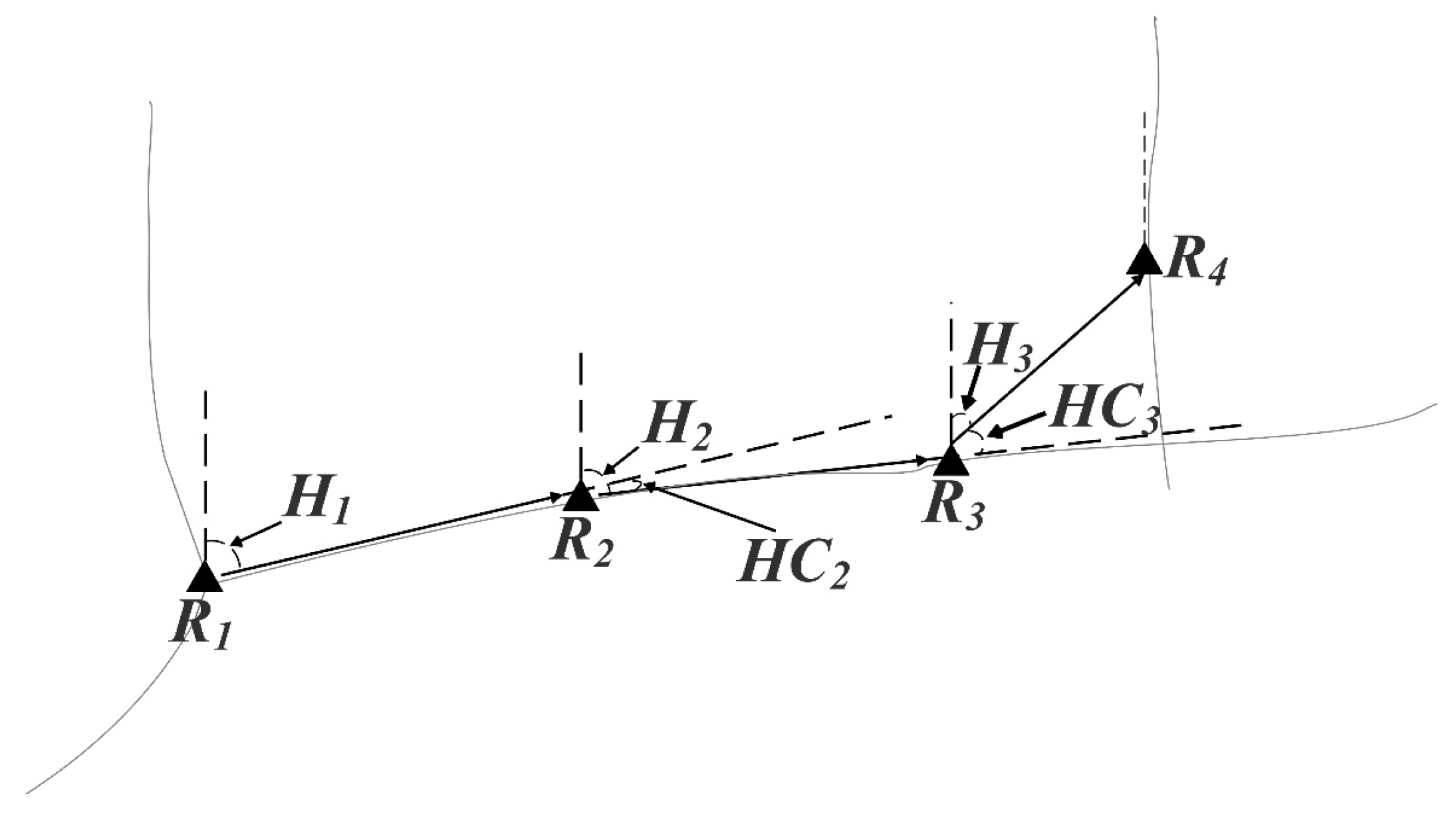
3.1. Trajectory Features Definition

The ‘actual’ trajectory is subject to the driver’s driving experience and road traffic conditions. Based on the definition of the anomalous trajectory (Section 1.2), we must consider the differences between the ‘actual’ trajectory and the ‘optimal’ trajectory, including velocity, distance, turns, and intersections. The ‘optimal’ trajectory in our work is the shortest route between the same source-destination pair. There are significant differences between the actual trajectory and the shortest route in terms of distance and intersection. We can define two trajectory features to quantify these differences: the route selection ($RS$) feature and the intersection rate ($IR$) feature. Due to the lack of sample point information for the shortest route, we are unable to obtain the velocity of the sample point and the turn differences between the sample points. In addition, studies have found that a trajectory of excessive turning or frequent velocity changes is anomalous [24,28]. Therefore, we define three trajectory features to quantify the difference between the velocity-related and turn measures: the heading change rate ($\mathrm{HCR}$) feature, the slow point rate ($\mathrm{SPR}$) feature, and the velocity change rate ($\mathrm{VCR}$) feature.

We suppose that a trajectory $R$ is composed of a series of $n$ points in a time series, which can be expressed as $R=\left\{R_1,R_2,\dots ,R_n\right\}=\left\{\left(x_1,y_1,t_1\right),\left(x_2,y_2,t_2\right),\dots ,\left(x_n,y_n,t_n\right)\right\}$. For the trajectory data, we can obtain N different trajectories, most of which have different source and destination points. The values of five trajectory features are directly represented by $RS$, $IR$, $\mathrm{HCR}$, $\mathrm{SPR}$, and $\mathrm{VCR}$.

Definition 1.

Route selection ($RS$).

Due to considerations such as distance and cost, the driver has multiple choices of trajectory routes based on the same source and destination. Considering that the driver’s income is related to distance, the shortest route could be the driver’s optimal choice. The route selection feature ($RS$) is used to qualitatively determine the difference between the actual route ($L_{ar}$) and the shortest route ($L_{sr}$), as shown in Figure 3a. $L_{ar}$ is the actual length of the trajectory, and $L_{sr}$ is the length of shortest distance route from the same source point to the destination point. In urban areas, the shortest route is computed with reference to so-called generalized costs [29]. In our work, we consider the length of the trajectory as the cost and obtain the shortest distance route. The method uses the Dijkstra algorithm [44].

$$RS=\frac{\left|L_{ar}-L_{sr}\right|}{L_{ar}}$$

(1)

The range of $RS$ is 0 to 1. If the difference between the actual route and the shortest route is greater, then $RS$ is close to 1, thus showing that the actual route selection might be a detour behavior compared with the shortest route. Otherwise, $RS$ is close to 0.

Definition 2.

Intersection rate feature ($IR$).

The intersection is a basic component of road networks and usually has complex traffic conditions such as traffic lights and traffic congestion. When the long-term trajectory passes through a large number of intersections, it is possible to encounter these traffic conditions. Therefore, we use the intersection ratio feature to quantify the difference between the intersection number of the actual route ($N_{ar}$) and the intersection number of the shortest route ($N_{sr}$), as shown in Figure 3a.

$$IR=\{\begin{array}{ll}\frac{\left|N_{ar}-N_{sr}\right|}{N_{ar}+ N_{sr}},& N_{ar}\ne 0\\ 0,& N_{ar}=0 and N_{sr}=0\\ 1,& N_{ar}=0 and N_{sr}\ne 0\end{array}$$

(2)

Normally, the value of $IR$ is between 0 and 1. If the difference between the actual route and the shortest route is greater, $IR$ is close to 1; otherwise, $IR$ is close to 0. However, there are two special cases for the feature, as shown in Figure 3b. When $N_{ar}$ is 0 and $N_{sr}$ is 0, the actual route is exactly the same as the shortest route. When $N_{ar}$ is 0 and $N_{sr}$ is not 0, the actual route is on a ring road or the shortest route has road restrictions, which means that the actual route has a high probability of including a detour. According to the meaning of $IR$, we set $N_{ar}$ to 0 and 1 respectively.

Definition 3.

Heading change rate feature ($\mathrm{HCR}$).

A turn is one of the most basic movements. A trajectory has many turns that can represent an anomalous trajectory, such as forming a detour, a loop, or intensive turns. In the GNSS trajectory data, we use the north direction as the reference direction; the angle between two consecutive sample points and the north direction is calculated as the heading direction of the trajectory segment. The heading change is defined as the heading direction difference between two continuous trajectory segments and can be used to express the turn behavior of the trajectory.

Suppose there is a trajectory $R$ of $n$ points $R=\{R_1,R_2,\dots ,R_n$}, $R_i, i=\left(1,2,\dots ,n\right),$ including the source-destination pair and sample points. The heading directions of $R_i$ are $H_i,i=\left(2,3,\dots ,n\right)$, as shown in Figure 4. The threshold of the heading change is $H_t$, and the heading change of $R_i$ is $H{C}_i=\left|H{C}_i-H{C}_{i-1}\right|, i=\left(2,3,\dots ,n-2\right)$. The heading change rate $\mathrm{HCR}$ is defined as follows:

$$f_{\mathrm{HCR}}\left(H{C}_i\right)=\{\begin{array}{cc}1,& H{C}_i\ge H_t\\ 0,& H{C}_i<H_t\end{array},with$$

$$\mathrm{HCR}=\frac{{{\displaystyle \sum }}_{i=2}^{n-2}{f}_{\mathrm{HCR}}\left(H{C}_i\right)}{n-2}$$

(3)

The range of $\mathrm{HCR}$ is 0 to 1. If the actual route has more turns, then the heading changes frequently and $\mathrm{HCR}$ is close to 1, thus showing that the actual route might be a detour or loop behavior. Otherwise, $\mathrm{HCR}$ is close to 0.

Definition 4.

Slow point rate feature ($\mathrm{SPR}$).

The slow points of the trajectory are those sample points for which the velocity is below a certain threshold. If the number of slow points is not high, traffic accidents or congestion may occur. When unexpected events happen, the slow points increase. Therefore, these continuous slow points reflect the area of unexpected events, as shown in Figure 5a.

Because the trajectory consists of a series of sample points, the instantaneous velocity of the sample point cannot reflect the actual movement of the trajectory. Therefore, we use the average velocity of the trajectory segment as the velocity of the current sample point ($V_i, i=\left(2,3,\dots ,n\right)$). The threshold of slow points is $S_t$. The slow point rate $\mathrm{SPR}$ is defined as follows:

$$f_{\mathrm{SPR}}\left(V_i\right)=\{\begin{array}{cc}1,& V_i\ge S_t\\ 0,& V_i>S_t\end{array},with$$

$$\mathrm{SPR}=\frac{{{\displaystyle \sum }}_{i=2}^n{f}_{\mathrm{SPR}}\left(V_i\right)}{n-1}$$

(4)

The range of $\mathrm{SPR}$ is 0 to 1. If traffic congestion or traffic accidents occur for a long time, the slow points of the trajectory will become greater and $\mathrm{SPR}$ is close to 1. Otherwise, $\mathrm{SPR}$ is close to 0.

Definition 5.

Velocity change rate feature ($\mathrm{VCR}$).

Velocity is one of the most basic features in the trajectory data. The velocity change feature records the number of unexpected events that occur during the movement of the trajectory. When the trajectory enters or stays away from the unexpected event area (see Definition 4 and Figure 5a), the velocity of two adjacent trajectory segments changes significantly, as shown in Figure 5b. The velocity of the current sample point is $V_i$. The threshold of velocity change is $V_t$, and the velocity change of $R_i$ is $V{C}_i=\left|V_i-V_{i-1}\right|, i=\left(2,3,\dots ,n-2\right)$. The velocity change rate $R_{vcr}$ is defined as follows:

$$f_{\mathrm{VCR}}\left(V{C}_i\right)=\{\begin{array}{cc}1,& V{C}_i\ge V_t\\ 0,& V{C}_i<V_t\end{array},with$$

$$CR=\frac{{{\displaystyle \sum }}_{i=2}^{n-2}{f}_{\mathrm{VCR}}\left(V{C}_i\right)}{n-2}$$

(5)

The range of $\mathrm{VCR}$ is 0 to 1. If traffic congestion or traffic accidents occur frequently, the velocity of the trajectory will change frequently and $\mathrm{VCR}$ is close to 1. Otherwise, $\mathrm{VCR}$ is close to 0.

3.2. Dempster-Shafer Evidence Theory

To combine the different trajectory features, we require the Dempster-Shafer (D-S) theory. The main purpose of this theory is to transform the uncertainty of a proposition into the uncertainty of a set, and evidence can be understood as a piece of information to support this proposition [45]. In our work, these trajectory features can be used as belief degrees from different sources to support trajectory anomalies and are finally combined to obtain the possible anomalies of all the actual trajectories.

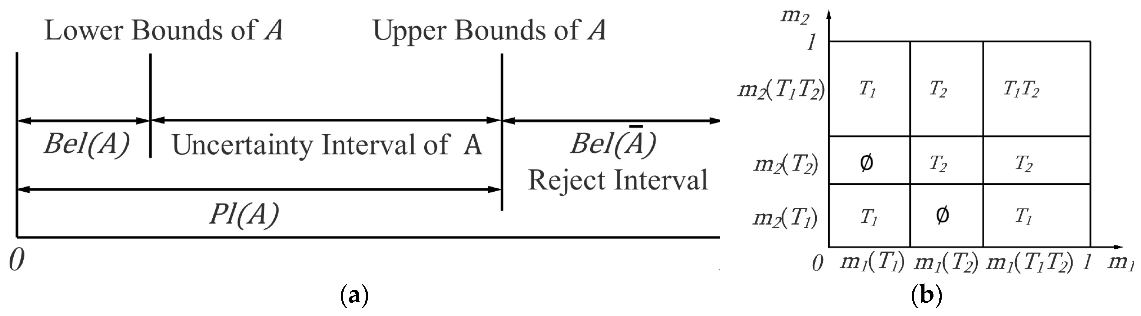
3.2.1. Theory Description

The Dempster-Shafer theory was proposed by Dempster in 1967 and further extended by Shafer [46]. The advantage of the theory includes two aspects: one is to directly express the uncertainly by assigning probability to the subset of a set; the other is to combine the bodies of evidence to derive new evidence. The basic definition and description are introduced below.

Definition 6.

Frame of discernment.

The frame of discernment $\mathsf{\Theta }$ is established to build a finite and non-empty set of mutually exclusive and exhaustive events.

$$\mathsf{\Theta }=\left\{T_1,T_2,\dots ,T_M\right\}$$

The power set is $2^{\mathsf{\Theta }}$ and contains all the possible subsets of $\mathsf{\Theta };$ $\varnothing$ is an empty set, where

$$2^{\mathsf{\Theta }}=\left\{\varnothing ,\left\{T_1\right\},\left\{T_2\right\},\dots ,\left\{T_M\right\},\left\{T_1,T_2\right\},\dots ,\left\{T_1,T_M\right\},\dots ,\left\{T_1,T_2,\dots ,T_j\right\},\dots ,\mathsf{\Theta }\right\}$$

Definition 7.

Hypothesis.

When $A$ is an element of the power set of $\mathsf{\Theta }$ and $A\in 2^{\mathsf{\Theta }}$, $A$ is defined as a hypothesis or proposition. For example, $A=\left\{T_1,T_2\right\}$ or $A=\left\{T_1,T_2,\dots ,T_j\right\}$.

Definition 8.

Mass function or basic probability assignment (BPA).

The mass function ($m:2^{\mathsf{\Theta }}$), also called a basic probability assignment (BPA) or basic belief, is defined to satisfy Equation (6), and $m\left(A\right)$ describes the support degree for hypothesis $A$. $\varphi$ is the empty set, and m is evidence to support hypothesis $A$. Usually, the BPA can be achieved by testing data or expert experiences.

$$m:2^{\mathsf{\Theta }}\to \left[0,1\right]\{\begin{array}{c}{\displaystyle {\displaystyle \sum }_{A\in 2^{\mathsf{\Theta }}}}m\left(A\right)=1\\ m\left(\varphi \right)=0\end{array}$$

(6)

When $m\left(A\right)=0$, hypothesis $A$ lacks any believability. A value of $m\left(A\right)$ between [0,1] indicates partial belief, and $A$ is called a focal element of $\mathsf{\Theta }$. The focal element and its BPA constitute the binary body ($A,m\left(A\right)$) as the evidence body, and the evidence is composed of several evidence bodies.

Definition 9.

Belief function ($Bel$) and plausibility function ($Pl$).

$$Bel\left(A\right)={\displaystyle {\displaystyle \sum }_{B\subseteq A}}m\left(B\right),with$$

$$\mathrm{Pl}\left(A\right)=1-\mathrm{Bel}\left(\overline{A}\right)={\displaystyle {\displaystyle \sum }_{B\cap A\ne \varphi }}m\left(B\right)$$

(7)

Finally, the belief function ($Bel$) and plausibility function ($Pl$) are defined in Equation (7) to describe the uncertainty of hypothesis $A$, where $\overline{A}$ is the complement set of $A$ such that $\overline{A}=\mathsf{\Theta }-A$. As shown in Figure 6, $Bel\left(A\right)$ is a measure of the total amount of true beliefs in evidence m for hypothesis $A$, and $Pl\left(A\right)$ describes the unsuspicious possibility to support hypothesis $A$. The interval $\left[Bel\left(A\right),Pl\left(A\right)\right]$ can be interpreted as the lower and upper bounds of the probability.

3.2.2. Dempster’s Combinational Rule

Definition 10.

Two-evidence combination.

In fact, there is a lot of evidence supporting Hypothesis T. Dempster’s combinational rule is provided to combine the mass values of evidence. Suppose there are two evidences, $E_1$ and $E_2$, which belong to the same frame of discernment $\mathsf{\Theta }$, and their corresponding basic probability assignments (BPAs) are denoted by $m_1$ and $m_2$. $B$ and $C$ are the corresponding hypothesis sets of $2^{\mathsf{\Theta }}$. The evidences $E_1$ and $E_2$ are composed of hypothesis sets $B$ and $C$ and their corresponding BPAs. Dempster’s combinational rule is represented as follows:

$$m_{1\oplus 2}\left(A\right)=\{\begin{array}{cc}\frac{1}{1-k}{\displaystyle {\displaystyle \sum }_{B\cap C=A}}m1\left(B\right)m2\left(C\right),& A\ne \varnothing \\ 0,& A=\varnothing \end{array},with$$

$$k={\displaystyle {\displaystyle \sum }_{B\cap C=\varnothing }}m1\left(B\right)m2\left(C\right)$$

(8)

In the above equations, $1/\left(1-k\right)$ is the normalized factor. $k$ reflects the degree of conflict among evidence. When $k=0$, the two evidences are fully compatible with each other. In contrast, when $k=1$, the two evidences are in conflict with each other. $\oplus$ is called the direct sum of operation.

To illustrate the synthesis of $m_1$ and $m_2$, we suppose that $\mathsf{\Theta }=\left\{T_1,T_2\right\}$; then, $B,C$ include three focal elements, $\left\{T_1\right\},\left\{T_2\right\},\left\{T_1,T_2\right\}$, and their BPAs are $m_1\left(T_1\right)$, $m_1\left(T_1\right)$, $m_1\left(T_1{T}_2\right)$, $m_2\left(T_1\right)$, $m_2\left(T_2\right)$, and $m_2\left(T_1{T}_2\right)$. As shown in Figure 6b, the largest rectangle represents the total reliability. The BPAs of $m_1$ and $m_2$ in their respective corresponding focal elements are represented by horizontal and vertical lines, respectively. The measure of the small rectangle is then generated by the intersection of the vertical line and the horizontal line, $m_1\left(T_i\right)m_2\left(T_j\right),i,j=\left(1,2,3\right)$, which indicates the reliability assigned to both $T_i$ and $T_j$. Suppose $A=\left\{T_1\right\}$. If we want to calculate the value of $m_{1\oplus 2}\left(A\right)$, we must only select the rectangles containing only $T_1$ in Figure 6b. The values of these rectangles are multiplied by two BPAs containing local element $T_1$. Then, we add them together and normalize them. Apparently, Dempster’s combinational rule is commutative and assigns the mass of the empty set to each set through the use of normalization.

Definition 11.

N evidence combination.

We suppose N is independent, the reliable pieces of evidence are $E_1,E_2,\dots ,E_N$, their BPAs are $m_1,m_2,\dots ,m_N$ separately obtained, and their local elements are $A_i$. The order and grouping of the combinations need not be considered because Dempster’s combinational rule is commutative and associative. The rule can be defined as follows:

$$m\left(A\right)=\{\begin{array}{cc}{m}_1\oplus m_2\oplus \dots m_N=\frac{1}{1-k}{\displaystyle {\displaystyle \sum }_{\cap A_i=A}}{\displaystyle {\displaystyle \prod }_{1\le i\le N}}{m}_i\left(A_i\right),& A\ne \varnothing \\ 0,& A=\varnothing \end{array},$$

$$with k={\displaystyle {\displaystyle \sum }_{\cap T_i=\varnothing }}{\displaystyle {\displaystyle \prod }_{1\le i\le N}}{m}_i\left(A_i\right)$$

(9)

There will be conflicts between the evidence due to the deviation of observation and subjective judgment. Therefore, there are many new evidence combination rules, such as Yager’s rule [47] and Murphy’s rule [48]. However, none has thus far been accepted as a standard method.

3.3. Trajectory Anomaly Hypothesis

Our study considers the two-class problem of whether an extracted trajectory $R$ is normal or anomalous. Thus, the frame of discernment is formed and contains two possibilities because $\mathsf{\Theta }=\left\{N,A\right\}$, where $\left\{N\right\}$ means trajectory $R$ is normal, and $\left\{A\right\}$ means $R$ is anomalous. The power set of $\mathsf{\Theta }$ has three hypotheses, $\left\{N\right\}$, $\left\{A\right\}$, and {$N,A$}, where $\left\{N,A\right\}$ means that it is impossible to determine whether $R$ is normal or anomalous.

After we have identified the frame of discernment and the three hypotheses, we need experts or statistics to determine the basic probability assignment (BPA) of the different hypotheses based on the requirements of the D-S evidence theory. In this paper, for a trajectory, we have acquired its five trajectory features, which are considered as observations of whether the trajectory is anomalous. Therefore, we treat the five trajectory features as experts and then give their respective BPAs for the three hypotheses. The evidence for the trajectory is defined as follows.

Definition 12.

The evidence for the trajectory.

Suppose $F_i,i=(1,2,3,4,5)$ is value of five trajectory features, where $F_i\in (RS,IR,\mathrm{HCR},\mathrm{SPR},\mathrm{VCR})$. According to the definition in Section 3.2, when $F_i$ is larger, there is a greater possibility that the trajectory is anomalous. For the three hypotheses $\left\{N\right\}$, $\left\{A\right\}$, {$N,A$}, when $F_i\ne 0$, we set $m_i\left(A\right)=F_i$ and $m_i\left(N\right)=1-F_i$. When $F_i=0$, trajectory $R$ is normal, then $m_i\left(N\right)=F_i$. The three hypotheses and their BPAs constitute the evidence for the trajectory. Five trajectory features correspond to their BPAs, represented by the symbols $m_i,i=\left(1,2,3,4,5\right)$. Each feature assumes the corresponding $m_i\left(A\right)$, $m_i\left(N\right)$ and $m_i\left(A,N\right)$ for the three trajectory anomalies. It constitutes evidence of the trajectory. Our goal is to combine these five evidences to get new BPAs based on Equations (8) and (9), that is $m_1\oplus m_2\oplus m_3\oplus m_4\oplus m_5$.

The sum of the BPAs of the evidence should be equal to 1, such that $m\left(A\right)+m\left(N\right)+m\left(A,N\right)=1$. The BPA structure of evidence for the trajectory is set as shown in

Table 1. The BPA structure of evidences for a trajectory.

	${\mathit{m}}_{\mathit{i}}\left(\mathit{N}\right)$	${\mathit{m}}_{\mathit{i}}\left(\mathit{A}\right)$	${\mathit{m}}_{\mathit{i}}\left(\mathit{N},\mathit{A}\right)$
$F_i\ne 0$	$1-F_i-0.05$	$F_i$	0.005
$F_i=0$	$1-F_i-0.01$	0.005	0.005

. When the BPA of the evidence has a value of 0, the result of the combination according to Dempster’s combinational rule is 0, which results in a failure to correctly judge the anomalous result of the trajectory. Therefore, we set $m\left(N,A\right)=0.005$ and $m\left(A\right)=0.005$ to help avoid judgement errors caused by conflicts of evidence.

After combining different evidence based on Dempster’s combinational rule, we can acquire the uncertainty internal $\left[Bel\left(A\right),Pl\left(A\right)\right]$ for each trajectory. Because $Bel\left(A\right)$ and $Pl\left(A\right)$ indicate the lower and upper bounds of probability that the trajectory is anomalous, we can define the anomalous decision rules as follows.

Definition 13.

Anomalous decision rules.

When $Bel\left(A\right)\ge 0.5$, the trajectory can be defined as anomalous. For other uncertain cases, we can combine the time information to make an auxiliary judgment. For example, if the $Bel\left(A\right)$ of the trajectory is in the range of 0.4 to 0.5 and the time is midnight, the trajectory can be judged to be anomalous.

4. Experiment of the Proposed Approach

4.1. Data Pre-Processing and Trajectory Extraction

In this paper, taxi trajectories are used. They include nearly 20,000 taxis and come from a local institution in Wuhan City, China, on 1 May 2014. The dataset is recorded as a series of points over 24 h at least once every 60 s and includes some spatial and attribute information, such as location, speed, direction, passenger state, and engine state.

Table 2. Sample records from taxi trajectory data.

Vehicle ID	Time	Longitude	Latitude	Direction	ACC	State
0001	00:10:05	114 ****	30 ****	122	On	empty
0002	00:10:05	114 ****	30 ****	NULL	On	heave
0003	00:10:05	114 ****	30 ****	NULL	Off	empty
…	…	…	…	…	…	…
0001	00:11:05	114 ****	30 ****	NULL	On	heave
0002	00:11:05	114 ****	30 ****	55	On	empty
0003	00:10:05	114 ****	30 ****	10	On	heave

provides a sample record. Longitudes and latitudes are shown as ‘****’ to protect privacy. Each trajectory point includes location and time information, as well as some attribute information, such as ‘Direction’, ‘ACC’, and ‘State’. The ‘Direction’ represents the direction of the taxi. This value is more a default and cannot be used. ‘Acc’ represents the state of the engine. The ‘On’ value means that the engine is working, and the ‘OFF’ value means that the engine is in flameout. The ‘State’ represents whether there are passengers in the taxi. The ‘heave’ value means that the taxi has passengers, and the ‘empty’ value means that there are no passengers in the taxi.

Because of the drift of GNSS devices or their incorrect use by taxi drivers, the raw data contain wrong points that must be removed by data filtering through experience. For example, the distances of some points are far beyond the distance that a taxi could drive in one minute. Some error points can be removed through experience, for example, when the value of ‘State’ is ‘heave’, the value of ‘Acc’ must be ‘On’. Those records for which the value of ‘ACC’ is ‘Off’ are errors.

In order to extract the trajectory, we need to sort the Vehicle IDs to obtain the trajectory point sequence of each vehicle in 24 h. Based on the ‘ACC’ and ‘State’ information, the trajectory can be divided into three types of sub-trajectories: no-service trajectory, passenger trajectory, and passenger-seeking trajectory. The no-service trajectory is composed of points with an ‘Off’ value of ‘ACC’, which represents the position of the driver’s rest and is not applicable to the study in this paper. The passenger-seeking trajectory is generated by the driver looking for passengers. Most of these trajectories contain only one or two points, which does not meet the requirements of this experiment. Therefore, the experimental trajectory used in this paper is the passenger trajectory.

A passenger trajectory consists of the successive pick-up point and drop-off point and the sample points between them. The pick-up point is the point where the ‘ACC’ value is ‘On’ and the ‘State’ value has ‘empty’ to ‘heave’. In Table 2, the point on the fourth line is the pick-up point of vehicle 0001. The drop-off point is the point where the ‘ACC’ value is ‘On’ and the ‘State’ value has ‘heave’ to ‘empty’. In Table 2, the point on the fifth line is the pick-up point of vehicle 0002. Otherwise, the GPS drift problem will lead to an inaccurate positioning of the taxi trajectory data. Thus, matching taxi trajectory data to the current road network is necessary. In our study, the map-matching method is based on the nearest principle. First, we need to determine the search radius, obtain the buffer area and candidate road segments of the point to be matched, and then we calculate the distance between the point to be matched and each candidate road segment. Finally, we select the first three candidate road segments with the shortest distance. The matching road section is determined according to the road number of the previous matching point.

The dataset contains 36,955 passenger trajectories. These trajectories are overlaid with a Wuhan city road map, as shown in Figure 7a. Due to the low sampling rate of the trajectory data, we cannot obtain the actual route between the two sample points. In this study, we use the shortest route between the two sample points to establish the actual route for the calculation of the following trajectory features, as shown in Figure 7b. After processing, the trajectory is completely displayed along the road, which is shown in a small box in Figure 7.

4.2. Parameter Selection and Combination Analysis

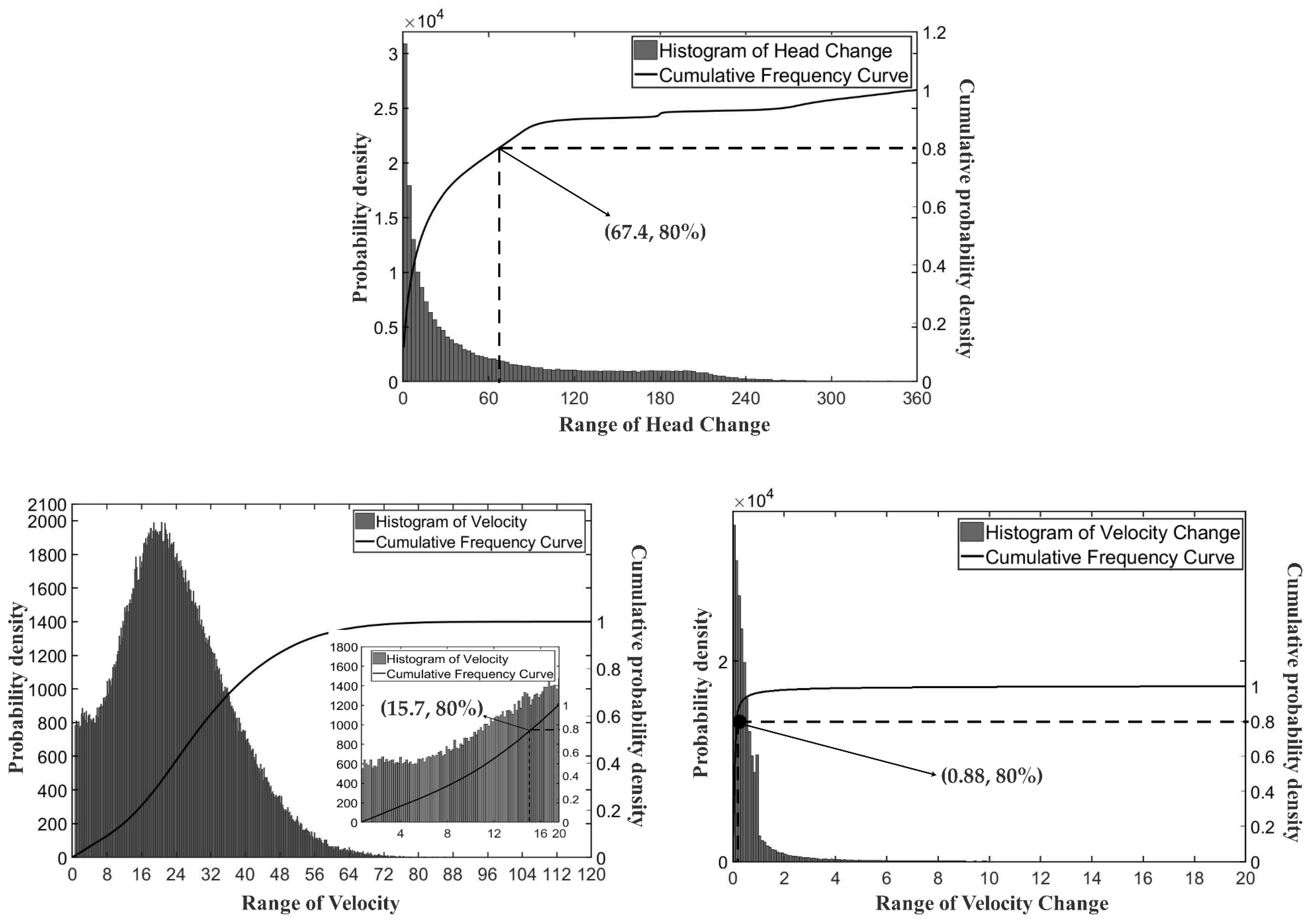
4.2.1. Parameter Selection for $\mathrm{HCR}$, $\mathrm{SPR}$ and $\mathrm{VCR}$

There are two approaches for the selection of parameters: First, when there are training data, by calculating the results in a certain parameter interval and comparing with the real result, the parameters that correspond to the best results are selected. Zheng et al. [49] defined accuracy by segment and accuracy by distance to validate the effectiveness of each feature. Second, when there are no training data, most parameters are given fixed values based on expert experience. Huang et al. [24] defined the features in relation to the combination of turns and the need for a threshold to remove trivial turns. He directly assigned the threshold to 30 degrees based on experience.

In this study, the three parameters $H_t$, $S_t$ and $V_t$ correspond to the three trajectory features $\mathrm{HCR}$, $\mathrm{SPR}$ and $\mathrm{VCR}$. These parameters are certain values that should be given based on expert experience. For example, if the velocity of the point is less than 10m/s, we consider it as a slow point. However, because the road network structure and related speed limit information are inconsistent, the trajectory data from different regions are different. We must determine the parameters of the trajectory features based on the trajectory data.

The histogram and cumulative frequency curve of $\mathrm{HCR}$, $\mathrm{SPR}$ and $\mathrm{VCR}$ are shown in Figure 8. The x-axis is in intervals according to the feature values, the left y-axis is the trajectory number in the interval, and the right y-axis is the cumulative percentage of the trajectory numbers. $\mathrm{HCR}$ and $\mathrm{VCR}$ are consistent with the long-tailed distribution, and $\mathrm{SPR}$ is a Gaussian distribution that can also be viewed as a combination of long-tailed distributions. Using an 80/20 rule of thumb, for such a long-tailed distribution, the majority of the occurrences are accounted for by the first 20% of items in the distribution. In other words, when the feature values are sorted from small to large, the first 20% of values occupy 80% of the trajectory numbers. The value of the x-axis corresponding to the right y-axis value of 0.8 is the threshold we want to determine. For $\mathrm{HCR}$ and $\mathrm{VCR}$, the values of $H_t$ and $V_t$ are 67.4 degrees and 0.88 m/s, respectively. For $\mathrm{SPR}$, we focus on the lesser value; thus, we choose the left half of its distribution as the long-tailed distribution to choose the threshold. The value of $S_t$ is 15.7 km/h.

4.2.2. Combination Analysis of Trajectory Feature

For the D-S evidence theory, each trajectory feature is equivalent to an observation of the discernment frame $\mathsf{\Theta }=\left\{\left\{N\right\},\left\{A\right\},\left\{N, A\right\}\right\}$. Different combinations of features or which features are selected will affect the recognition results. To verify the effect of these combinations or selections on the results, we denote the five trajectory features $IR,RS,\mathrm{HCR},\mathrm{SPR},\mathrm{VCR}$ and then select 2, 3, 4, and 5 features and infer anomalous trajectories according to Dempster’s combinational rule and anomalous decision rules. The different combinations of features are shown in

Table 3. The different combinations of trajectory features.

Index	2 Features	Index	3 Features	Index	4 Features	Index	5 Features
1	($IR,RS$)	11	($IR,RS,\mathrm{HCR}$)	21	($IR,RS,\mathrm{HCR},\mathrm{SPR}$)	26	($IR,RS,\mathrm{HCR},\mathrm{SPR},\mathrm{VCR}$)
2	($IR,\mathrm{HCR}$)	12	($IR,RS,\mathrm{SPR}$)	22	($IR,RS,\mathrm{HCR},\mathrm{VCR}$)
3	($IR,\mathrm{SPR}$)	13	($IR,RS,\mathrm{VCR}$)	23	($IR,RS,\mathrm{SPR},\mathrm{VCR}$)
4	($IR,\mathrm{VCR}$)	14	($IR,\mathrm{HCR},\mathrm{SPR}$)	24	($IR,\mathrm{HCR},\mathrm{SPR},\mathrm{VCR}$)
5	($RS,\mathrm{HCR}$)	15	($IR,\mathrm{HCR},\mathrm{VCR}$)	25	($RS,\mathrm{HCR},\mathrm{SPR},\mathrm{VCR}$)
6	($RS,\mathrm{SPR}$)	16	($IR,\mathrm{SPR},\mathrm{VCR}$)
7	($RS,\mathrm{VCR}$)	17	($RS,\mathrm{HCR},\mathrm{SPR}$)
8	($\mathrm{HC}R,\mathrm{SPR}$)	18	($RS,\mathrm{HCR},\mathrm{VCR}$)
9	($\mathrm{HCR},\mathrm{VCR}$)	19	($RS,\mathrm{SPR},\mathrm{VCR}$)
10	($\mathrm{SPR},\mathrm{VCR}$)	20	($\mathrm{HCR},\mathrm{SPR},\mathrm{VCR}$)

. The combination analysis of trajectory features will help to verify the rationality of our proposed five trajectory features.

To verify the combination of trajectory features, we must mark some anomalous trajectories based on the trajectory data. We obtained 272 trajectories that select the same source and destination points in our experimental trajectories, and manually marked 6 anomalous trajectories according to the definition of the anomalous trajectory. According to the 26 combinations of trajectory features provided in Table 3, we obtained the $Bel\left(A\right)$ value of each trajectory according to Equation (7), and finally obtained anomalous trajectories according to the anomalous decision rule. To validate the effectiveness of the results, we focused on accuracy with $Recall$, $Precision$, and $F1\text{-}Score$.

$$Recall=\frac{m}{N}$$

(10)

$$recision=\frac{m}{M}$$

(11)

$$F1\text{-}Score=2\times Recall\times \frac{Precision}{Recall+Precison}$$

(12)

where $M$ denotes the total number of anomalous trajectories being predicted, $N$ stands for the total number of anomalous trajectories being classified, and m denotes the number of anomalous trajectories being correctly predicted. In fact, $Recall$ and $Precision$ are contradictory in some cases. Therefore, the $F1\text{-}Score$ is the weighted average of $Recall$, and $Precision$ and is used to determine the results.

Overall, inference accuracy changes across the different combinations of trajectory features, as shown in Figure 9. When $Precision$ is high, $Recall$ is correspondingly lower, that is, the changes in $Recall$ and $Precision$ generally tend to be mostly opposite. As shown by the red box in Figure 9 when only two features are combined, the maximum value of $F1\text{-}Score$ is 0.667. When three features are combined, the maximum value of $F1\text{-}Score$ is 0.75. When four features are combined, the maximum value of $F1\text{-}Score$ is 0.8. When five features are combined, the maximum value of $F1\text{-}Score$ is 0.923. As the participation features increase, the accuracy of the result increases. Therefore, the judgment of our anomalous trajectories requires the combination of five trajectory features.

4.3. Anomalous Trajectory Results and Analysis

After calculating these trajectory features, we obtained the $Bel\left(A\right)$ of the trajectory according to Equation (7). We sorted the values of $Bel\left(A\right)$ and inferred that trajectories with $Bel\left(A\right)\ge 0.5$ are anomalous. Because $Bel\left(A\right)$ is in the range of 0.4 to 0.5, we can infer that trajectories are anomalous if these trajectories occur between 10 pm and 7 am the following morning.

4.3.1. Comparison with Clustering Method

We used 272 trajectories that selected the same source and destination points in our experimental trajectories. The geographic distribution of these trajectories is shown in Figure 10a. We inferred 7 anomalous trajectories according to the proposed D-S evidence theory. In addition, many of the trajectories were similar; as shown in Figure 10a, there were four cluster centers and four normal trajectory clusters could be acquired. To compare with the results of our method, we also detected 9 anomalous trajectories according to the trajectory clustering method proposed by Wang et al. [12]. The two anomalous trajectories are the color lines in Figure 10b,c, respectively. The trajectory clustering method considers the similarity between trajectories and clusters trajectories with large similarities; those trajectories that deviate from these clusters are defined as anomalous trajectories. As shown in Figure 10d, the results of the two methods show that there are 6 identical anomalous trajectories and that there are 1 and 3 different anomalous trajectories. The dashed lines are the different trajectories obtained by the trajectory clustering, and the solid line is the different trajectory obtained using our method.

The five features of the four trajectories (1, 2, 3 and 4) are shown in Figure 10d. Trajectory 1 is recognized as a normal trajectory according to the trajectory clustering method because it is highly similar to the blue trajectory (Figure 10a). The $\mathrm{VCR}$ and $\mathrm{SPR}$ of trajectory 1 are large, indicating that the velocity changes significantly and there are many slow points. According to our method, trajectory 1 can be identified as an anomalous trajectory. In addition, trajectories 2, 3, and 4 are recognized as anomalous trajectories using the trajectory clustering method. The $\mathrm{VCR}$ and $\mathrm{SPR}$ of these trajectories are small, indicating that the velocity is stable. According to our method, these trajectories are not anomalous trajectories. The generation of the trajectory is definitely affected by other trajectories and road conditions. The anomalous trajectory obtained using the trajectory clustering method considers the interaction between the trajectories. When the anomalous trajectory is treated as an independent individual, and the optimal route from the source point to the destination point may itself be congested or detoured, this will cause some trajectories to be misjudged. In addition, the clustering method is limited to the data set from the same source-destination pair. Conversely, our method can determine whether such a trajectory is anomalous and is not limited to a single source-destination pair.

4.3.2. Statistical Analysis of the Anomalous Trajectory

We used all 36,955 trajectories from our experimental data. Some statistical information is shown in

Table 4. The statistical information of anomalous trajectories and all real trajectories.

	Trajectory Numbers	Average Time (min)	Average Lengths (km)	Average $\mathit{R}\mathit{S}$	Average $\mathit{I}\mathit{R}$	Average $\mathrm{HCR}$	Average $\mathrm{SPR}$	Average $\mathrm{VCR}$
Anomalous Trajectories	408	5.731	2.005	0.551	0.564	0.605	0.502	0.546
Normal Trajectories	36,547	6.882	3.549	0.068	0.111	0.208	0.207	0.196
All Trajectories	36,955	6.869	3.532	0.073	0.067	0.131	0.034	0.278

, in which the number of anomalous trajectories is 408, which is 1.1% of all the trajectories. Thus, these trajectories are on the low side. The average time and length of anomalous trajectories are smaller than the average time and length of all trajectories, which indicates that anomalous trajectories are not trajectories with a larger time or length. This also shows that anomalous trajectories cannot be detected using simple time and length statistics. In contrast, the five average features of the anomalous trajectories exceed 0.5 and are much larger than the average features of normal trajectories and all trajectories, which is consistent with the principles of our method.

The anomalous trajectories in Table 4 are clearly distinguished from all trajectories in length, time, and five features. However, the average can only indicate the amount of trend in the dataset. To further illustrate the differences between anomalous trajectories and normal trajectories, we used box plots to show them. To show the effect, we normalized the lengths and time of the trajectory, as shown in Figure 11. The anomalous trajectories and the normal trajectories are similar in length and time distribution and are clearly different in the five features. In other words, an anomalous trajectory and a normal trajectory cannot be distinguished only by their length and time statistics. In addition, the five features of the trajectory can clearly distinguish between the anomalous trajectory and the normal trajectory. However, the judgement of the anomaly cannot be inferred using simple statistics, because there are also smaller features in the anomalous trajectories. Similarly, there are also larger features in the normal trajectories. For this case, a specific example of an anomalous trajectory is described below.

4.4. Anomalous Trajectory Interpretation

The geographic distributions of anomalous trajectories are represented in Figure 12. Here, changes in the blue color depth indicate the times of the trajectories: light-colored trajectories are relatively short, and dark-colored trajectories are relatively long. The lengths of these trajectories are tagged on the map. Some trajectories are located outside the urban area of Wuhan and are displayed in the small box in the upper-left corner of Figure 12.

There are four examples to explain our results and show the plausibility of values. Each example includes a pair of anomalous trajectories and normal trajectories that are similar in some trajectory features, as shown in Figure 13, in which the black solid line is the anomalous trajectory or a normal trajectory. The black dotted line is the shortest route. The five features of the trajectory are also shown in the figure. To clearly show the movement of the trajectory, we moved the overlapping trajectories to each side of the road.

In the first example, the source and destination points are on the same road and are not far from each other, which is manifested in the large $RS$ and $IR$ features (shown in Figure 13a). Due to the closeness of the source and destination points, such trajectories are primarily likely to be requested by passengers to go to a certain place and return to the source point. However, it should be noted that all loop routes are considered as anomalous trajectories; their difference lies in the $\mathrm{SPR}$ and $\mathrm{VCR}$ features. These two features are large, indicating that special events occur on the road. Therefore, in Figure 13a, the left trajectory is inferred to be an anomalous trajectory, and the right trajectory is considered as normal.

The second example is the obvious detour behavior of the driver, which is manifested in the large $RS$, $IR$ and $\mathrm{HCR}$ features (shown in Figure 13b). The source and destination points of the trajectory are not on the same road. A passenger whose destination is unfamiliar will most likely not discover that the driver is making a detour. Of course, it is also possible that the shortest route is temporary inaccessible. At this time, $\mathrm{SPR}$ and $\mathrm{VCR}$ are very important. If these two features of the ‘actual’ trajectory are large and $Bel\left(A\right)$ exceeds 0.5 after the combination of evidence, the trajectory is inferred to be an anomalous trajectory; otherwise, it is considered as normal.

The third example is a trajectory caused by traffic conditions on the road network, such as traffic accidents and traffic congestion, which are manifested in the large $\mathrm{SPR}$, $\mathrm{VCR}$ and $\mathrm{HCR}$ features (shown in Figure 13c). The difference between the left trajectory and right trajectory is that the $IR$ features are different, indicating that the left trajectory passes more intersections than its corresponding shortest route. Therefore, for a driver who encounters traffic situations, if the driving has more intersections, the left trajectory is inferred to be an anomalous trajectory, and the right trajectory is normal.

The fourth example is the trajectory with little difference between the ‘actual’ trajectory and the shortest route, that is, the $RS$ of the trajectory is small. There are two types of such trajectories; one is when the actual trajectory is on the same road as the shortest route, and the other is the trajectory shown in Figure 13d. The $\mathrm{SPR}$, $\mathrm{VCR}$ and $\mathrm{HCR}$ of the left trajectory and the right trajectory are similar, but the $IR$ features are different. This results in the left trajectory being inferred to be anomalous, whereas the right trajectory is considered as normal. Similar trajectories are also judged to be anomalous, but their problems might be caused by other features.

5. Discussion

In this paper, we define the characteristics of the ‘optimal’ trajectory from the source point to the destination point. The difference between the ‘actual’ trajectory and the ‘optimal trajectory’ can be observed using the trajectory feature. These trajectory features describe anomalies in the trajectory. As seen in Figure 11, the five features of each trajectory actually have different trends. In fact, each feature is an observation of one aspect of the anomalous trajectory. For example, the $RS$ feature can identify the trajectories of detours, and the $\mathrm{VCR}$ feature can acquire trajectories in which some special events occur. The trajectory inferred from a single feature might be inaccurate and redundant. For example, long-sequence trajectories remain at high speeds and are not necessarily anomalous. Therefore, we fuse these trajectory features to obtain the anomaly probability of each trajectory to infer the anomalous trajectory more accurately.

Lacking the attribute information and semantic information of the road, we use the shortest route from the source point to the destination point as the geometrically ‘optimal’ trajectory in the road network. Due to the low sampling rate of our trajectory data, the shortest route we obtained cannot acquire the sampling points of the intermediate process. This limitation leads us to consider only the variation of the ‘actual’ trajectory when defining the trajectory velocity and direction-related features; thus, the three related features $\mathrm{HCR}$, $\mathrm{SPR}$ and $\mathrm{VCR}$ are defined. If the trajectory data-sampling rate is high, such as one point per second, then the feasible method is to divide the geographic space into grids and convert the ‘actual’ trajectory and the ‘optimal’ trajectory into grid sequences. Based on this method, different related features of the trajectory can be further defined. Overall, the five trajectory features are defined based on the characteristics of our trajectory data, which are suitable for trajectory data with a low sampling rate. The low data-sampling rate results in some methods that are not suitable for our data.

The D-S evidence theory provides a method to fuse evidence. There are many methods for data fusion, including Bayesian estimation, neural networks, and expert systems. These methods require a large number of samples to be trained to meet the accuracy requirements. However, there is no such anomalous attribute information in the taxi trajectory data, and the number of trajectories is large; thus, it is difficult to judge manually. The D-S evidence theory does not require prior knowledge. The most important problem to consider in the use of the evidence theory is the evidence in conflict, including two aspects. One is the conflict of the evidence itself. In our study, each feature change is different, which will inevitably lead to conflicts and a decrease in the possibility of anomalies. When that possibility falls below 0.5, we define these trajectories as being in an acceptable range. We can thus filter out trajectories that are not very clear and obtain more accurate anomalous trajectories. The second is the conflict of evidence 0. According to Table 1, we change these 0 features to reduce judgement errors caused by this conflict.

We consider the five features of a trajectory as different evidence to observe the anomaly of the trajectory and combine such evidence based on Dempster’s combinational rule. In this paper, we consider that each type of evidence has the same influence on the final anomalous results; that is, the weight of different evidence is the same when it is combined. However, in practice, different evidence has different effects on the results. The $\mathrm{HCR}$ feature should have the greatest effect as evidence when it is necessary to monitor driver fraud behavior. The purpose of this paper is to comprehensively consider these five evidences to infer the anomalous trajectories strictly. Certainly, we can consider assigning different weights to the evidence according to different application requirements.

The time complexity of a trajectory feature calculation depends upon the number of sampling points of a trajectory. The time sampling rate of the trajectory is one minute, so the number of sampling points in most trajectories is approximately ten, and it takes approximately five seconds to calculate all the features of a trajectory. In addition, the time complexity of our method depends upon the number of trajectories. When the amount of data is large, we consider dividing the trajectories into multiple groups and calculating these features in parallel.

The aim of this paper is to recognize anomalous trajectories based on the D-S evidence theory by considering driving behavior and road network constraints. In traditional methods, the density and similarity of population trajectories are used to define normal and anomalous objects. In this paper, the multi-feature fusion of a single trajectory is used as the criterion for judging anomalies. Each trajectory is independent of any other. The inference of an anomalous trajectory focuses on real-time performance. The research object of this study is a single trajectory. As long as a trajectory is formed, we can make a judgment as to whether it is anomalous. Therefore, our method applies not only to historical trajectories but also to online inference.

We have given four examples of a comparison of anomalous trajectories with normal trajectories. These examples contain some special trajectories that are similar in some features. As in Example 2, some studies can find driver fraud behavior [25] but cannot distinguish between the two trajectories in Figure 13b. Similarly, for the loop trajectories in Example 1, we can filter them more carefully through other features. Our method cannot only infer the anomalous trajectories of various examples but also has a more refined ability to detect and a higher probability of detecting anomalous trajectories. Of course, due to the lack of contextual information, our method requires a greater number of relevant features for further inferring anomalous trajectories.

6. Conclusions and Future Research

In this paper, we proposed an automatic inference method for the new selection of anomalous trajectories based on the D-S evidence theory by considering driving behavior and road network constraints. We used five trajectory features that reflect trajectory shape and attribution information: $RS$, $IR$, $\mathrm{HCR}$, $\mathrm{SPR}$, and $\mathrm{VCR}$. Dempster’s combinational rule from the D-S evidence theory was used to fuse the trajectory features. We defined the BPA of the features and the rule of judging the anomalous trajectories. The experimental results show that these anomalous trajectories are not the long-distance and high-time trajectories, which is different from people’s intuitive impression. This result was largely determined by the definition of the anomalous trajectory in this paper. We have listed four examples to illustrate the plausibility of the results. The main contribution of this paper is to consider the trajectories of different S-D pairs when more accurately discovering anomalous trajectories; the method can effectively perform automatic mode inference using taxi GNSS trajectories. Moreover, our method is for a single trajectory and does not limit the influence of other trajectories. It is suitable for the real-time monitoring of anomalous trajectories and can effectively monitor driving behavior.

Future research suggested by our paper includes the following aspects: (1) in the current study, the weight of each feature is the same when the trajectory features are fused as evidence. However, the purpose of inferring anomalous trajectories is occasionally different, such as specifically targeting driver fraud behavior. Therefore, in future research, the weight of the features can be modified according to different application scenarios to meet the requirements for anomalous trajectory refinement; (2) This study employed historical taxi trajectory data. However, anomaly judgment of trajectories requires not only effectiveness but also real-time operation. In future research, we will infer anomalous trajectories based on real-time GNSS trajectory data and perform the inference and analysis of anomalies online; (3) The experimental data did not include prior expert knowledge of anomalies; moreover, we did not consider other data for calculating the features, such as basic geographic information, traffic status data, or driver income information. This information could improve the accuracy of anomalous trajectory judgments and should be more conducive to explaining the cause of the anomalous trajectory. This point is a key consideration for our follow-up research.

References

1. Liu, X.; Ban, Y. Uncovering Spatio-Temporal Cluster Patterns Using Massive Floating Car Data. ISPRS Int. J. Geo-Inf. 2013, 2, 371–384. [Google Scholar] [CrossRef] [Green Version]
2. Veloso, M.; Phithakkitnukoon, S.; Bento, C. Urban mobility study using taxi traces. In Proceedings of the 2011 International Workshop on Trajectory Data Mining and Analysis, Beijing, China, 18 September 2011; pp. 23–30. [Google Scholar]
3. Matsubara, Y.; Li, L.; Papalexakis, E.; Lo, D.; Sakurai, Y.; Faloutsos, C. F-Trail: Finding Patterns in Taxi Trajectories. In Proceedings of the Pacific-Asia Conference on Knowledge Discovery and Data Mining, Gold Coast, Australia, 14–17 April 2013; pp. 86–98. [Google Scholar]
4. Owens, J.; Hunter, A. Application of the self-organising map to trajectory classification. In Proceedings of the Third IEEE International Workshop on Visual Surveillance, Dublin, Ireland, 1 July 2000. [Google Scholar]
5. Foresti, G.L.; Mahonen, P.; Regazzoni, C.S. Multimedia Video-Based Surveillance Systems: Requirements, Issues, and Solutions; Springer US: New York, NY, USA, 2000. [Google Scholar]
6. Marcenaro, L.; Oberti, F.; Foresti, G.L.; Regazzoni, C.S. Distributed architectures and logical-task decomposition in multimedia surveillance systems. Proc. IEEE 2001, 89, 1419–1440. [Google Scholar] [CrossRef]
7. Saul, H.; Junghans, M.; Leich, A. Identifying Hazardous Locations at Intersections by Automatic Traffic Surveillance. Available online: https://uknowledge.uky.edu/cgi/viewcontent.cgi?referer=https://www.google.com/&httpsredir=1&article=2069&context=ktc_researchreports (accessed on 20 September 2018).
8. Detzer, S.; Junghans, M.; Kozempel, K.; Saul, H. Analysis of traffic safety for cyclists: The automatic detection of critical traffic situations for cyclists. In Proceedings of the 20th International Conference on Urban Transport and the Environment, Faro Algarve, Portugal, 28–30 May 2004; pp. 491–503. [Google Scholar]
9. Junghans, M.; Kozempel, K.; Saul, H. Chances for the evaluation of the traffic safety risk at intersections by novel methods. J. Sci. Pract. Econ. 2015, 1. Available online: https://elib.dlr.de/95641/1/2015_Chances%20for%20the%20evaluation%20of%20the%20traffic%20safey%20risk%20at%20intersections%20by%20novel%20methods%20(Journal%20Transport%20Rossiskoi%20Federazii).pdf (accessed on 20 September 2018).
10. Li, Z.; Filev, D.P.; Kolmanovsky, I.; Atkins, E.; Lu, J. A new clustering algorithm for processing GPS-based road anomaly reports with a mahalanobis distance. IEEE Trans. Intell. Transp. Syst. 2017, 18, 1980–1988. [Google Scholar] [CrossRef]
11. Chen, Q.; Qiu, Q.; Li, H.; Wu, Q. A neuromorphic architecture for anomaly detection in autonomous large-area traffic monitoring. In Proceedings of the International Conference on Computer-Aided Design, San Jose, CA, USA, 18–21 November 2013; pp. 202–205. [Google Scholar]
12. Wang, Y.; Qin, K.; Chen, Y.; Zhao, P.X. Detecting Anomalous Trajectories and Behavior Patterns Using Hierarchical Clustering from Taxi GPS Data. ISPRS Int. J. Geo-Inf. 2018, 7, 25. [Google Scholar] [CrossRef]
13. Zhang, D.; Li, N.; Zhou, Z.; Chen, C.; Sun, L.; Li, S. iBAT: detecting anomalous taxi trajectories from GPS traces. In Proceedings of the 13th International Conference on Ubiquitous Computing, Beijing, China, 17–21 September 2011; pp. 99–108. [Google Scholar]
14. Chen, C.; Zhang, D.; Castro, P.S.; Li, N.; Sun, L.; Li, S.; Wang, Z. iBOAT: Isolation-Based Online Anomalous Trajectory Detection. IEEE Trans. Intell. Transp. Syst. 2013, 14, 806–818. [Google Scholar] [CrossRef]
15. Zhou, Z.; Dou, W.; Jia, G.; Hu, C.; Xu, X.; Wu, X.; Pan, J. A method for real-time trajectory monitoring to improve taxi service using GPS big data. Inf. Manag. 2016, 53, 964–977. [Google Scholar] [CrossRef]
16. Lee, J.G.; Han, J.; Li, X. Trajectory Outlier Detection: A Partition-and-Detect Framework. In Proceedings of the 2008 IEEE 24th International Conference on Data Engineering, Cancun, Mexico, 7–12 April 2008; pp. 140–149. [Google Scholar]
17. Liu, L.; Qiao, S.; Zhang, Y.; Hu, J. An efficient outlying trajectories mining approach based on relative distance. Int. J. Geogr. Inf. Sci. 2012, 26, 1789–1810. [Google Scholar] [CrossRef]
18. Lei, P.R. A framework for anomaly detection in maritime trajectory behavior. Knowl. Inf. Syst. 2016, 47, 189–214. [Google Scholar] [CrossRef]
19. Zhu, J.; Jiang, W.; Liu, A.; Liu, G.; Zhao, L. Effective and efficient trajectory outlier detection based on time-dependent popular route. World Wide Web 2016, 20, 111–134. [Google Scholar] [CrossRef]
20. Li, X.; Han, J.; Kim, S. Motion-Alert: Automatic Anomaly Detection in Massive Moving Objects. In Proceedings of the International Conference on Intelligence and Security Informatics, San Diego, CA, USA, 23–24 May 2006; pp. 166–177. [Google Scholar]
21. Yang, W.; Gao, Y.; Cao, L. TRASMIL: A local anomaly detection framework based on trajectory segmentation and multi-instance learning. Comput. Vis. Image Underst. 2013, 117, 1273–1286. [Google Scholar] [CrossRef] [Green Version]
22. Liu, L.X.; Qiao, S.J.; Liu, B.; Le, J.J.; Tang, C.J. Efficient trajectory outlier detection algorithm based on R-Tree. J. Softw. 2009, 20, 2426–2435. [Google Scholar]
23. Han, B.; Wang, Z.; Jin, B. An anomaly detection algorithm for taxis based on trajectory data mining and online real-time monitoring. J. Univ. Sci. Technol. China 2016, 46, 247–252. (In Chinese) [Google Scholar]
24. Huang, H. Anomalous behavior detection in single-trajectory data. Int. J. Geogr. Inf. Sci. 2015, 29, 2075–2094. [Google Scholar] [CrossRef]
25. Ge, Y.; Xiong, H.; Liu, C.; Zhou, Z.H. A Taxi Driving Fraud Detection System. In Proceedings of the 2011 IEEE 11th International Conference on Data Mining, Vancouver, BC, Canada, 11–14 December 2012; pp. 181–190. [Google Scholar]
26. Zhou, Y.; Fang, Z.X.; Li, Q.Q.; Guo, S. Anomalous Taxi Trajectory Detection Based on Experiential Constraint Rules and Evidence Theory. Geomat. Inf. Sci. Wuhan Univ. 2016, 41, 797–802. Available online: http://ch.whu.edu.cn/CN/abstract/abstract5466.shtml (accessed on 20 September 2018). (In Chinese).
27. Chen, Q.; Whitbrook, A.; Aickelin, U.; Roadknight, C. Data classification using the Dempster-Shafer method. J. Exp. Theor. Artif. Intell. 2014, 26, 493–517. [Google Scholar] [CrossRef]
28. Ge, Y.; Liu, C.; Xiong, H.; Chen, J. A taxi business intelligence system. In Proceedings of the 17th ACM SIGKDD International Conference on Knowledge Discovery and Data Mining, San Diego, CA, USA, 21–24 August 2011; pp. 735–738. [Google Scholar]
29. Hanssen, T.E.S.; Mathisen, T.A.; Jørgensen, F. Generalized Transport Costs in Intermodal Freight Transport. Procedia-Soc. Behav. Sci. 2012, 54, 189–200. [Google Scholar] [CrossRef] [Green Version]
30. Das, R.; Winter, S. Detecting Urban Transport Modes Using a Hybrid Knowledge Driven Framework from GPS Trajectory. ISPRS Int. J. Geo-Inf. 2016, 5, 207. [Google Scholar] [CrossRef]
31. Sadilek, A.; Kautz, H. Recognizing multi-agent activities from GPS data. In Proceedings of the Twenty-Fourth AAAI Conference on Artificial Intelligence, Atlanta, GA, USA, 11–15 July 2010; pp. 1134–1139. [Google Scholar]
32. Zhao, X.; Cheng, X.; Zhou, J.; Xu, Z.; Dey, N.; Ashour, A.S.; Satapathy, S.C. Advanced Topological Map Matching Algorithm Based on D-S Theory. Arab. J. Sci. Eng. 2017, 43, 3863–3874. [Google Scholar] [CrossRef]
33. Xiao, G.; Juan, Z.; Zhang, C. Travel mode detection based on GPS track data and Bayesian networks. Comput. Environ. Urban Syst. 2015, 54, 14–22. [Google Scholar] [CrossRef]
34. Pang, L.X.; Chawla, S.; Liu, W.; Zheng, Y. On detection of emerging anomalous traffic patterns using GPS data. Data Knowl. Eng. 2013, 87, 357–373. [Google Scholar] [CrossRef] [Green Version]
35. Essa, I. Gaussian process regression flow for analysis of motion trajectories. In Proceedings of the IEEE International Conference on Computer Vision, Barcelona, Spain, 6–13 November 2011; pp. 1164–1171. [Google Scholar]
36. Ye, F.; Chen, J.; Li, Y.B. Improvement of DS Evidence Theory for Multi-Sensor Conflicting Information. Symmetry 2017, 9, 69. [Google Scholar] [Green Version]
37. Dymova, L.; Sevastjanov, L. An interpretation of intuitionistic fuzzy sets in terms of evidence theory: Decision making aspect. Knowl. Based Syst. 2010, 23, 772–782. [Google Scholar] [CrossRef]
38. Dong, G.; Kuang, G. Target Recognition via Information Aggregation Through Dempster-Shafer’s Evidence Theory. IEEE Geosci. Remote Sens. Lett. 2015, 12, 1247–1251. [Google Scholar] [CrossRef]
39. Talavera, A.; Aguasca, R.; Galván, B.; Cacereño, A. Application of Dempster-Shafer theory for the quantification and propagation of the uncertainty caused by the use of AIS data. Reliab. Eng. Syst. Saf. 2013, 111, 95–105. [Google Scholar] [CrossRef]
40. Kong, Q.; Chen, Y.; Liu, Y. An improved evidential fusion approach for real-time urban link speed estimation. In Proceedings of the Intelligent Transportation Systems Conference, Seattle, WA, USA, 30 September–3 October 2007; pp. 562–567. [Google Scholar]
41. Zhang, N.; Xu, J.; Lin, P.Q.; Zhang, M. An approach for real-time urban traffic state estimation by fusing multisource traffic data. In Proceedings of the 10th World Congress on Intelligent Control and Automation, Beijing, China, 6–8 July 2012; pp. 4077–4081. [Google Scholar]
42. Baloian, N.; Frez, J.; Pino, J.A.; Zurita, G. Efficient Planning of Urban Public Transportation Networks. In Proceedings of the International Conference on Ubiquitous Computing and Ambient Intelligence, Puerto Varas, Chile, 1–4 December 2015; pp. 439–448. [Google Scholar]
43. De Souza, R.P.; Carmo, L.F.R.C.; Pirmez, L. An enhanced bootstrap method to detect possible fraudulent behavior in testing facilities. Accredit. Qual. Assur. 2017, 22, 21–27. [Google Scholar] [CrossRef]
44. Johnson, D.B. A Note on Dijkstra’s Shortest Path Algorithm. J. ACM 1973, 20, 385–388. [Google Scholar] [CrossRef]
45. Zhou, D.; Wei, T.; Zhang, H.; Ma, S.; Wei, F. An Information Fusion Model Based on Dempster-Shafer Evidence Theory for Equipment Diagnosis. ASCE-ASME J. Risk Uncertain. Eng. Syst. 2018, 4. [Google Scholar] [CrossRef]
46. Shafer, G. A Mathematical Theory of Evidence; Princeton University Press: Princeton, NJ, USA, 1976. [Google Scholar]
47. Yager, R.R.; Liu, L. Classic Works of the Dempster-Shafer Theory of Belief Functions; Springer: Berlin, Germany, 2010. [Google Scholar]
48. Murphy, C.K. Combining belief functions when evidence conflicts. Decis. Support Syst. 2000, 29, 1–9. [Google Scholar] [CrossRef]
49. Zheng, Y.; Li, Q.; Chen, Y.; Xie, X.; Ma, W.Y. Understanding mobility based on GPS data. In Proceedings of the International Conference on Ubiquitous Computing, Seoul, Korea, 21–24 September 2008; pp. 312–321. [Google Scholar]
Figure 1. The ‘optimal’ trajectory (a) and ‘actual’ trajectory (b) from the source point to the destination point.
Information 09 00258 g001
Figure 2. A process for the anomalous trajectory inference method.
Information 09 00258 g002
Figure 3. (a) Diagram of the route selection feature and the intersection rate feature. (b) Two special cases for the intersection rate feature.
Information 09 00258 g003
Figure 4. Calculation of the heading change rate feature based on GNSS trajectories.
Information 09 00258 g004
Figure 5. (a) Diagram of the slow points rate. (b) Diagram of the velocity change rate.
Information 09 00258 g005
Figure 6. (a) The relationship of the belief function and the plausibility function. (b) The synthesis of m 1 and m 2 based on Dempster’s combinational rule.
Information 09 00258 g006
Figure 7. (a) The geographic distribution of trajectories used in the experiment. (b) The geographic distribution of the processed trajectories used in the experiment.
Information 09 00258 g007
Figure 8. The histogram and cumulative frequency curve of HCR , SPR , and VCR .
Information 09 00258 g008
Figure 9. The inference is performed based on different combinations of features.
Information 09 00258 g009
Figure 10. (a) The geographic distribution of trajectories. (b) The anomalous trajectories based on our method. (c) The anomalous trajectories based on the trajectory clustering method. (d) The comparison of anomalous trajectories between two methods.
Information 09 00258 g010aInformation 09 00258 g010b
Figure 11. Box plot concerning trajectory distance, time, and five features. (a) The anomalous trajectories. (b) The normal trajectories.
Information 09 00258 g011
Figure 12. The geographic distributions of anomalous trajectories based on our method.
Information 09 00258 g012
Figure 13. The four examples of comparison between anomalous trajectory and normal trajectory.
Information 09 00258 g013