Article

Sensor Alignment for Ballistic Trajectory Estimation via Sparse Regularization

Unit 94, PLA 91550, Dalian 116023, China
*
Author to whom correspondence should be addressed.
Information 2018, 9(10), 255; https://doi.org/10.3390/info9100255
Submission received: 7 September 2018 / Revised: 11 October 2018 / Accepted: 16 October 2018 / Published: 18 October 2018
(This article belongs to the Section Information Processes)

Abstract

:
Sensor alignment plays a key role in the accurate estimation of the ballistic trajectory. A sparse regularization-based sensor alignment method coupled with the selection of a regularization parameter is proposed in this paper. The sparse regularization model is established by combining the traditional model of trajectory estimation with the sparse constraint of systematic errors. The trajectory and the systematic errors are estimated simultaneously by using the Newton algorithm. The regularization parameter in the model is crucial to the accuracy of trajectory estimation. Stein’s unbiased risk estimator (SURE) and general cross-validation (GCV) under the nonlinear measurement model are constructed for determining the suitable regularization parameter. The computation methods of SURE and GCV are also investigated. Simulation results show that both SURE and GCV can provide regularization parameter choices of high quality for minimizing the errors of trajectory estimation, and that our method can improve the accuracy of trajectory estimation over the traditional non-regularization method. The estimates of systematic errors are close to the true value.

1. Introduction

In the field of aerospace, an accurate trajectory is required for testing the performance of a new type of ballistic vehicle. Many sensors such as radars and telescopes are deployed to track the vehicle and collect the measurements of the trajectory. Then, these multi-sensor measurements are fused to acquire the optimal trajectory estimation [1,2,3,4]. Two types of errors exist in the measurements, affecting the accuracy of the trajectory estimation. The first are the random errors generated by the environmental noise. These errors fluctuate around zero randomly and cannot be removed. The second are the systematic errors that primarily originate from the misalignments of the sensor axes, the range offset errors, and the timing errors. Systematic errors lead the measurements to deviate from the true value with a constant or slowly varying amount, and thus can be removed. Sensor alignment aims at estimating and correcting the systematic errors by using the multi-sensor measurements. If these errors are not removed, a significant bias between the estimated trajectory and the true value can be caused, and consequently, the performance of trajectory estimation is degraded. Therefore, the sensor alignment is very important for improving the accuracy of ballistic trajectory estimation.
In the literature, there are typically two batch methods to address the sensor alignment for ballistic trajectory estimation: the error model best estimation of trajectory (EMBET) method [4] and the reduced parameter model (RPM) method [2,3,4,5]. The EMBET method estimates the trajectory and the systematic errors simultaneously using the least squares estimation. The drawback of this method is that the number of trajectory parameters to be estimated is very large, leading to low accuracy of trajectory estimation. The RPM method can be seen as an improvement of the EMBET method. In order to reduce the number of parameters to be estimated, the RPM method represents the trajectory by B-spline function. This paper is devoted to investigating the RPM method.
As the number of systematic errors to be estimated increases, the accuracy of the trajectory estimation of the RPM method can drop dramatically. Thus, this number should be decreased as much as possible by diagnosing which measurements have systematic errors. However, the diagnosis process needs the complicated man-machine conversation. In the area of signal processing, the sparse regularization is widely used for the reconstruction of sparse signals [6,7,8,9,10]. By appending the prior information of sparsity into the estimation model via a constraint term, the sparse regularization can overcome the ill-posedness of the model, and thus improves the performance of signal recovery. According to the historic data, only a few measurements contain systematic errors. Considering this property, Liu proposed a sensor alignment method based on the sparse regularization [11]. He modified the RPM method by adding a sparse constraint term on the systematic errors into the objective function. Then, the manual judgment on which measurements have systematic errors is omitted. However, to promote the performance of trajectory estimation, this regularization method requires the selection of a suitable regularization parameter, which is not studied in his paper. That is what we focus on. There are several methods for the selection of regularization parameters, e.g., L-curve method [12,13,14], Stein’s unbiased risk estimator (SURE) method [14,15,16,17], and general cross-validation (GCV) method [14,16,18,19,20]. The L-curve method considers the corner of an L-shaped curve (regularization term versus data misfit term) as the good parameter choice balancing the data misfit and the regularization errors. This method is non-convergent in a certain statistical sense and may choose a smaller parameter than the optimal one [14,21,22]. The SURE method chooses the regularization parameter by minimizing the SURE which is constructed as an unbiased estimator of predictive mean square error (MSE). For Gaussian noise, the SURE method can unbiasedly minimize the predictive MSE. However, this method requires the knowledge of noise variance. GCV is defined based on the principle that if one arbitrary data point is left out, the missing data can be predicted well by the solution from the residual data. The minimizer of GCV is determined as a suitable parameter choice. The advantage of the GCV method is that the noise variance is not required. However, this method does not have the unbiased property as does the SURE method. The GCV method can only asymptotically minimize the predictive MSE for specific regularization problems such as spline smoothing [18]. The SURE and GCV methods are developed for linear measurement models [14,15,16,17,18,19,20]. For the nonlinear model of trajectory estimation, the construction and computation of SURE and GCV are more complicated.
In this paper, we propose a sparse regularization based sensor alignment method involving the selection of a regularization parameter for ballistic trajectory estimation. The sparse regularization model is established by adding the sparse constraint of systematic errors into the traditional model of trajectory estimation. By solving this regularization model, the trajectory and the systematic errors are estimated simultaneously. SURE and GCV methods are used to choose an appropriate regularization parameter for optimizing the performance of trajectory estimation. The construction and computation of SURE and GCV under the nonlinear measurement model are investigated. The performance of our method is evaluated through a simulation experiment.

2. Estimates of Trajectory and Systematic Errors via Sparse Regularization

For a ballistic target, the trajectory x ( t ) = ( x ( t ) , y ( t ) , z ( t ) , x ˙ ( t ) , y ˙ ( t ) , z ˙ ( t ) ) T at time t includes the Cartesian components of the position (x(t),y(t),z(t)) and the velocity ( x ˙ ( t ) , y ˙ ( t ) , z ˙ ( t ) ) in the Earth-centered fixed coordinate system (ECF-CS). The measurement type of sensors involves azimuth, elevation, range, and range rate of target in the sensor’s East-North-Up coordinate system (ENU-CS). The detailed description of the ECF-CS and ENU-CS is given in [23]. The true azimuth A(t), elevation E(t), range R(t), and range-rate R ˙ ( t ) at time t can be computed by
{ A ( t ) = arctan ( y s ( t ) / x s ( t ) ) E ( t ) = arctan ( z s ( t ) / x s 2 ( t ) + y s 2 ( t ) ) R ( t ) = x s 2 ( t ) + y s 2 ( t ) + z s 2 ( t ) R ˙ ( t ) = x s ( t ) x ˙ s ( t ) + y s ( t ) y ˙ s ( t ) + z s ( t ) z ˙ s ( t ) x s 2 ( t ) + y s 2 ( t ) + z s 2 ( t )  
where (xs(t),ys(t),zs(t)) and ( x ˙ s ( t ) , y ˙ s ( t ) , z ˙ s ( t ) ) are the position and velocity of the target in the ENU-CS, which can be acquired by the ECF-to-ENU coordinate transformation of the trajectory x(t). Thus, the true measurements are nonlinear functions of the trajectory. Given the whole sampling moments t 1 , t 2 , , t M , let X = ( x ( t 1 ) T , x ( t 2 ) T , , x ( t M ) T ) T denote the vector of entire trajectory to be estimated and Y = ( y 1 , y 2 , , y n ) T denote a batch of n measurements of all sensors. Then, the nonlinear measurement model for trajectory estimation can be expressed as
Y = F ( X ) + E ( α ) + ε
where F ( X ) = ( f 1 ( X ) , f 2 ( X ) , , f n ( X ) ) T is the vector of true measurements as a nonlinear function of trajectory X, E ( α ) = ( e 1 ( α ) , e 2 ( α ) , , e n ( α ) ) T is the vector of systematic errors as a function of l systematic error coefficients α = ( α 1 , α 2 , , α l ) T , and ε = ( ε 1 , ε 2 , , ε n ) T is the vector of measurement noise. We assume that ε is an i.i.d zero-mean Gaussian random vector with the covariance matrix σ2I, i.e., εN(0,σ2I). In the ballistic target tracking system, the systematic errors of sensors are usually constant or drift very slowly. Consequently, E ( α ) is often a linear function of α .
The trajectory X can be represented by a B-spline function as follows [2]:
X
where B is a q by q matrix constructed by the B-spline bases, and θ = ( θ 1 , θ 2 , , θ q ) T is the vector of B-spline coefficients. Then, the measurement model (1) becomes
Y = F ( B θ ) + E ( α ) + T ( θ ) + ε
where T(θ) is the vector of errors caused by the fitting errors of B-spline function. The formula of T(θ) is unknown, but its value is very tiny. In the following paper, F ( B θ ) = ( f 1 ( B θ ) , f 2 ( B θ ) , , f n ( B θ ) ) T is abbreviated by F ( θ ) = ( f 1 ( θ ) , f 2 ( θ ) , , f n ( θ ) ) T . According to the RPM method, the estimation θ ^ and α ^ for θ and α can be obtained simultaneously by solving the following optimization problem:
( θ ^ T , α ^ T ) T = arg min θ , α | | Y F ( θ ) E ( α ) | | 2 2  
Then, the estimates of trajectory and systematic errors are given by X ^ = B θ ^ and E ^ = E ( α ^ ) .
If we know which measurements have systematic errors, the optimization problem (2) becomes
( θ ^ , α ^ I ) T = arg min θ , α I | | Y F ( θ ) E ( α I ) | | 2 2  
where αI is a subset of α indicating that the corresponding measurements contain systematic errors. Solving the optimization problem (3) instead of (2) can improve the accuracy of the trajectory estimation since the number of parameters to be estimated is reduced. However, we hardly know which measurements contain systematic errors beforehand in practice.
By analyzing the historical data, it is found that there are only a few measurements having the systematic errors, which means the systematic errors are sparse. The performance of trajectory estimation can be promoted by adding this prior information of sparsity as a constraint term into the optimization problem (2), i.e., constructing the following sparse regularization model:
( θ ^ λ T , α ^ λ T ) T = arg min θ , α | | Y F ( θ ) E ( α ) | | 2 2 + λ | | C α | | p p  
The first term in the right side of (4) is the data misfit term measuring the misfit between the model and the measurements. The second term is the regularization term or the constraint term measuring the sparsity of systematic errors. The lp-norm in (4) is defined as | | C α | | p p = ( i = 1 l | c i α i | p ) 1 / p where C is a l by l diagonal weighting matrix with positive diagonal elements ( c 1 , c 2 , , c l ) , and the constant p should satisfy 0 < p ≤ 1 for guaranteeing the sparsity of systematic errors. The diagonal weighting matrix C is used to lessen the gap in dimension between different measurement types. The large diagonal element in C should be chosen for the small dimension quantity of the corresponding measurement and vice versa. The regularization parameter λ is a positive constant which balances the misfit and the sparsity.
In the optimization problem (4), the lp-norm is non-differentiable around the origin when p ≤ 1. In order to apply the derivative based optimization method for finding the solution, we take the following smooth approximation for the lp-norm [14]:
| | C α | | p p i = 1 l ( ( c i α i ) 2 + δ ) p / 2
where δ is a small positive constant. Denoting β = ( θ T , α T ) T and β ^ λ = ( θ ^ λ T , α ^ λ T ) T , the optimization problem (4) is transformed into
β ^ λ = arg min β S ( β ) = arg min β | | Y F ( θ ) E ( α ) | | 2 2 + λ i = 1 l ( ( c i α i ) 2 + δ ) p / 2
Then, the above problem can be solved by the Newton algorithm [24] which has the following iteration formula:
β ^ λ ( i + 1 ) = β ^ λ ( i ) μ ^ H ( β ^ λ ( i ) ) 1 Γ ( β ^ λ ( i ) )  
where β ^ λ ( i ) is the solution obtained in the ith iteration, H(β) is the Hessian matrix H ( β ) = 2 S ( β ) / β 2 , Γ(β) is the gradient vector Γ ( β ) = S ( β ) / β , and μ ^ is given by
μ ^ = arg min μ S ( β ^ λ ( i ) μ H ( β ^ λ ( i ) ) 1 Γ ( β ^ λ ( i ) ) )
The iteration is terminated until the l2-norm of Γ(β) is close to zero. It can be seen that the smaller δ is, the closer β ^ λ is to the solution of the model (4). However, if δ is set to be too small, the number of iterations can be very large. We empirically choose δ = 1e-6 for a compromise between the accuracy of solution and the computational amount.
According to (5), we can get
Γ ( β ) = 2 ( M ( θ ) T ( Y F ( θ ) E ( α ) ) Q ( α ) T ( Y F ( θ ) E ( α ) ) 0.5 λ p C T W ( α ) C α )  
H ( β ) = 2 ( M ( θ ) T M ( θ ) M ( θ ) T Q ( α ) Q ( α ) T M ( θ ) Q ( α ) T Q ( α ) + 0.5 λ p C T D ( α ) C ) 2 ( k = 1 n ( y k f k ( θ ) e k ( α ) ) H k f ( θ ) 0 0 k = 1 n ( y k f k ( θ ) e k ( α ) ) H k u ( α ) )
where M ( θ ) = F ( θ ) / θ , Q ( α ) = E ( α ) / α , W ( α ) = diag ( w ( α 1 ) , w ( α 2 ) , , w ( α l ) ) , w ( α i ) = ( ( c i α i ) 2 + δ ) p / 2 1 , D ( α ) = diag ( d ( α 1 ) , d ( α 2 ) , , d ( α l ) ) , d ( α i ) = ( ( c i α i ) 2 + δ ) p / 2 2 ( ( p 1 ) ( c i α i ) 2 + δ ) , H k f ( θ ) = 2 f k ( θ ) / θ 2 , and H k u ( α ) = 2 e k ( α ) / α 2 . The second term in the right side of (7) can be omitted for reducing the computational complexity.

3. Regularization Parameter Selection
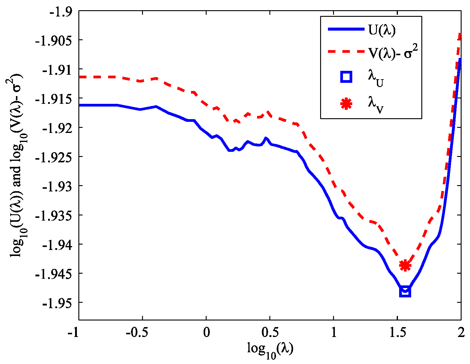
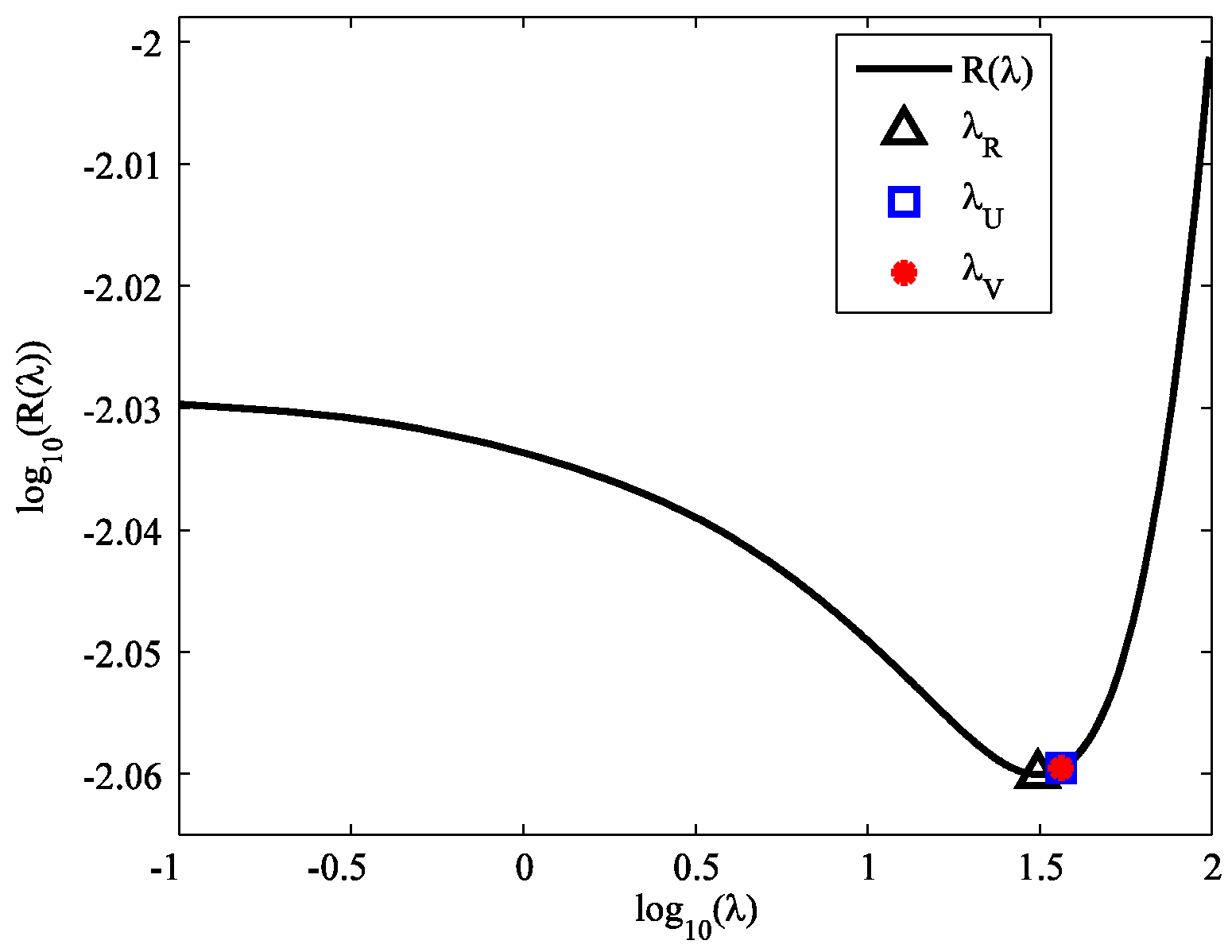
The solution of the regularization model depends on the regularization parameter λ. The small λ emphasizes the fitness between the model and the measurements, while the large λ emphasizes the prior information of systematic error sparsity. An appropriate λ should be chosen to balance the fitness and the sparsity. Two methods, SURE and GCV, are presented for selecting a regularization parameter in this section.

3.1. SURE Method

The SURE method attempts to find the optimal regularization parameter by minimizing the predictive MSE. Denoting g ( β ) = F ( θ ) + E ( α ) and g i ( β ) = f i ( θ ) + e i ( α ) , i = 1 , 2 , , n , the predictive MSE for the estimation β ^ λ is defined by
R ( λ ) = 1 n | | g ( β ^ λ ) F ( X ) E ( α ) | | 2 2
One may choose the parameter λ that minimizes R(λ). However, this strategy is infeasible since the true trajectory X and the true coefficients of systematic error α in (8) are unknown. Instead of directly minimizing R(λ), the SURE method determines the parameter λ by minimizing an unbiased estimator of R(λ). This estimator can be constructed by using the following theorem which is proposed by Stein [25].
Theorem 1.
Let Z = ( z 1 , z 2 , , z n ) T be an i.i.d Gaussian random vector with the mean ξ and the covariance matrix σ2I, i.e., Z~N(ξ2I), and P ( Z ) = ( p 1 ( Z ) , p 2 ( Z ) , , p n ( Z ) ) T be an almost differentiable function of Z for which
E i = 1 n | p i ( Z ) z i | <
Considering the estimate Z + P(Z) for ξ, we have
E | | Z + P ( Z ) ξ | | 2 2 = n σ 2 + E | | P ( Z ) | | 2 2 + 2 σ 2 i = 1 n E p i ( Z ) z i  
The unbiased estimator of the predictive MSE R(λ) is given by the following proposition:
Proposition 2.
Regard the estimate β ^ λ as an implicit function of the measurements Y = ( y 1 , y 2 , , y n ) T , and suppose that g ( β ^ λ ) = ( g 1 ( β ^ λ ) , g 2 ( β ^ λ ) , , g n ( β ^ λ ) ) T is almost differentiable for Y and satisfies E i = 1 n | g i ( β ^ λ ) / y i | < . Then, the random variable
U ( λ ) = σ 2 + 1 n | | Y g ( β ^ λ ) | | 2 2 + 2 σ 2 n tr ( g ( β ^ λ ) Y )  
is an unbiased estimator of R(λ).
Proof of Proposition 2.
According to (1), Y ~ N ( F ( X ) + E ( α ) , σ 2 I ) . From the assumptions in the proposition, we can conclude that g ( β ^ λ ) Y is also almost differentiable for Y and satisfies E i = 1 n | ( g i ( β ^ λ ) y i ) / y i | < . By using Theorem 1, we have
E R ( λ ) = 1 n E | | Y + g ( β ^ λ ) Y F ( X ) E ( α ) | | 2 2 = σ 2 + 1 n E | | Y g ( β ^ λ ) | | 2 2 + 2 σ 2 n i = 1 n E ( g i ( β ^ λ ) y i ) y i = σ 2 + 1 n E | | Y g ( β ^ λ ) | | 2 2 + 2 σ 2 n E tr ( g ( β ^ λ ) Y ) = E U ( λ )
Therefore, U(λ) is an unbiased estimator of R(λ). □
We call the estimator U(λ) SURE. The suitable regularization parameter λU can be found by minimizing the SURE, i.e., λ U = arg min λ U ( λ ) . We employ the golden section search to acquire λU. According to (9), we can see that the SURE method requires the knowledge of noise variance σ2.
Because g ( β ^ λ ) is an implicit function of Y, we cannot calculate g ( β ^ λ ) / Y directly. Since β ^ λ is the minimizer of S(β), we have
S ( β ) β | β = β ^ λ = 0  
By using the chain rule of derivation, we get
2 S ( β ) 2 β | β = β ^ λ β ^ λ Y + 2 S ( β ) β Y | β = β ^ λ = 0  
Thus,
β ^ λ Y = H ( β ^ λ ) 1 2 S ( β ) β Y | β = β ^ λ  
where H(β) is given by (7). According to (6), 2 S ( β ) / β Y in (10) has the following formula
2 S ( β ) β Y = 2 ( M ( θ ) Q ( α ) ) T  
By using the chain rule again, we have
g ( β ^ λ ) Y = g ( β ) β | β ^ λ β ^ λ Y  
where
g ( β ) β = ( M ( θ ) Q ( α ) )  
Finally, we obtain g ( β ^ λ ) / Y by submitting (10) into (11).

3.2. GCV Method

The GCV method is another popular strategy to determine the regularization parameter, which does not require the knowledge of noise variance. This method chooses the regularization parameter by minimizing the GCV, which is derived as a rotational invariant version of the ordinary cross-validation (OCV) [18]. The original GCV is designed for linear measurement models. We should construct the GCV adapting to the nonlinear measurement model of trajectory estimation.
The basic idea of OCV is that the estimation obtained by using the measurements with an arbitrary one left out will predict the missing one. Let Sk(β) be the objective function of (5) with the kth measurement yk omitted for k = 1 , 2 , , n , i.e.,
S k ( β ) = i k ( y i g i ( β ) ) 2 + λ i = 1 l ( ( c i α i ) 2 + δ ) p 2  
and β ^ λ k be the minimizer of Sk(β), i.e.,
β ^ λ k = arg min β S k ( β )  
Then, the OCV is defined as
V 0 ( λ ) = 1 n k = 1 n ( g k ( β ^ λ k ) y k ) 2  
Denote Y ˜ λ k = ( y 1 , y 2 , , y k 1 , g k ( β ^ λ k ) , y k + 1 , , y n ) T , and
S ˜ k ( β ) = | | Y ˜ λ k g ( β ) | | 2 2 + λ i = 1 l ( ( c i α i ) 2 + δ ) p 2 = i k ( y i g i ( β ) ) 2 + ( g k ( β ^ λ k ) g k ( β ) ) 2 + λ i = 1 l ( ( c i α i ) 2 + δ ) p 2
Let
β ˜ λ k = arg min β S ˜ k ( β )  
According to (12) and (13), we can infer that S ˜ k ( β ) S k ( β ) S k ( β ^ λ k ) = S ˜ k ( β ^ λ k ) . Thus,
β ^ λ k = arg min β S ˜ k ( β ) = β ˜ λ k
Then, we have g k ( β ^ λ k ) = g k ( β ˜ λ k ) for k = 1 , 2 , , n . By using the Taylor expansion, we can get the linearized approximation formula for g k ( β ^ λ k ) as follows:
g k ( β ^ λ k ) = g k ( β ˜ λ k ) g k ( β ^ λ ) + g k ( β ^ λ ) Y ( Y ˜ λ k Y ) = g k ( β ^ λ ) + g k ( β ^ λ ) y k ( g k ( β ^ λ k ) y k )
Then, we have
g k ( β ^ λ k ) y k g k ( β ^ λ ) y k 1 g k ( β ^ λ ) / y k  
Thus,
V 0 ( λ ) 1 n k = 1 n ( y k g k ( β ^ λ ) ) 2 ( 1 g k ( β ^ λ ) / y k ) 2  
Replacing g k ( β ^ λ ) / y k in the denominator of (14) by tr ( g ( β ^ λ ) / Y ) / n for the rotational invariant consideration as in [18], the GCV is defined as
V ( λ ) = 1 n | | Y g ( β ^ λ ) | | 2 2 ( 1 1 n tr ( g ( β ^ λ ) Y ) ) 2  
The computation method for g ( β ^ λ ) / Y is the same as SURE. Then, the regularization parameter determined by GCV is given by λ V = arg min λ V ( λ ) , which also can be solved through the golden section search.
The detailed construction and computation of SURE and GCV for the linear measurement model is given in [14]. Here, our SURE and GCV are able to manage the nonlinear measurement model of trajectory estimation, and the computation of SURE and GCV is more complicated than [14].

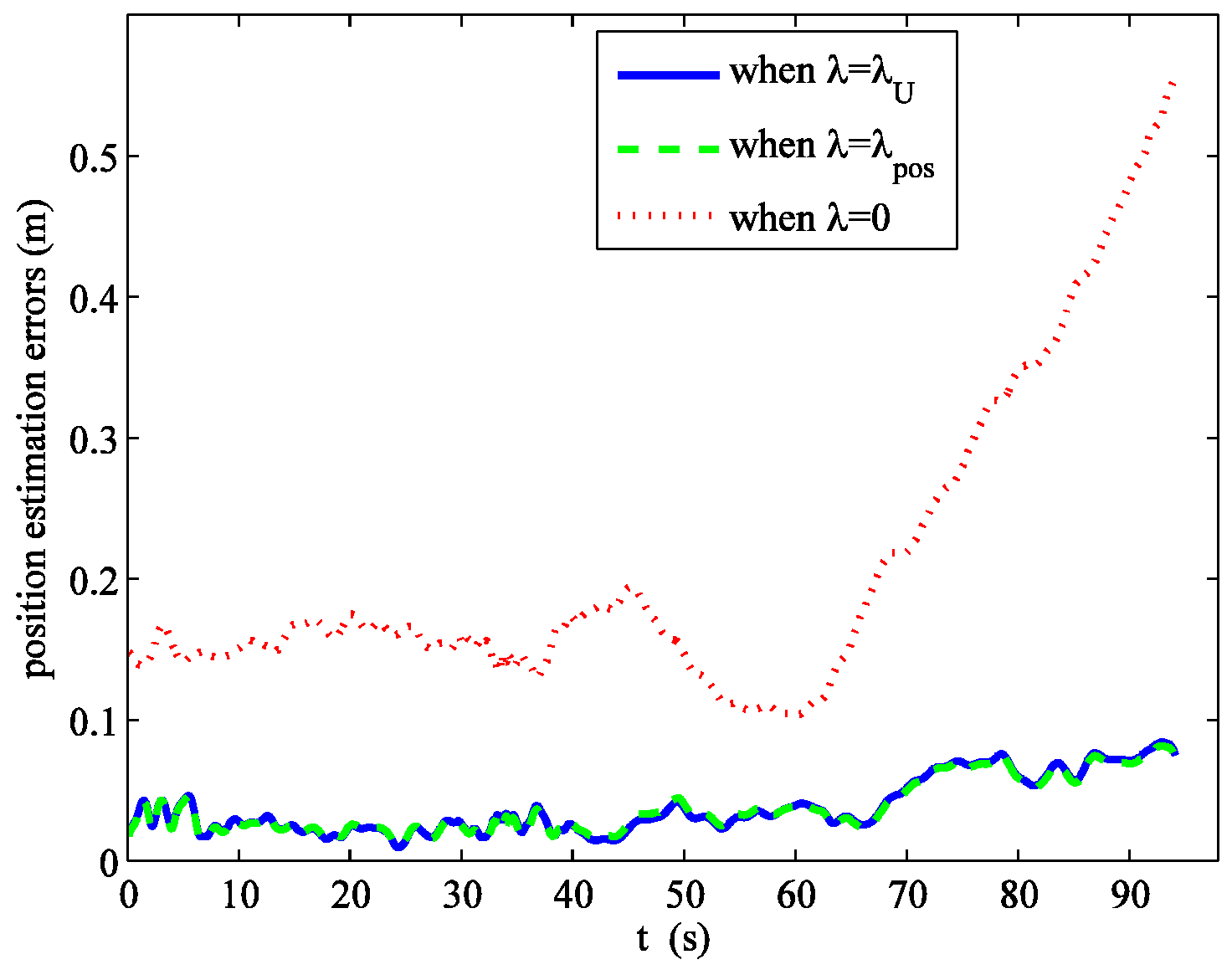
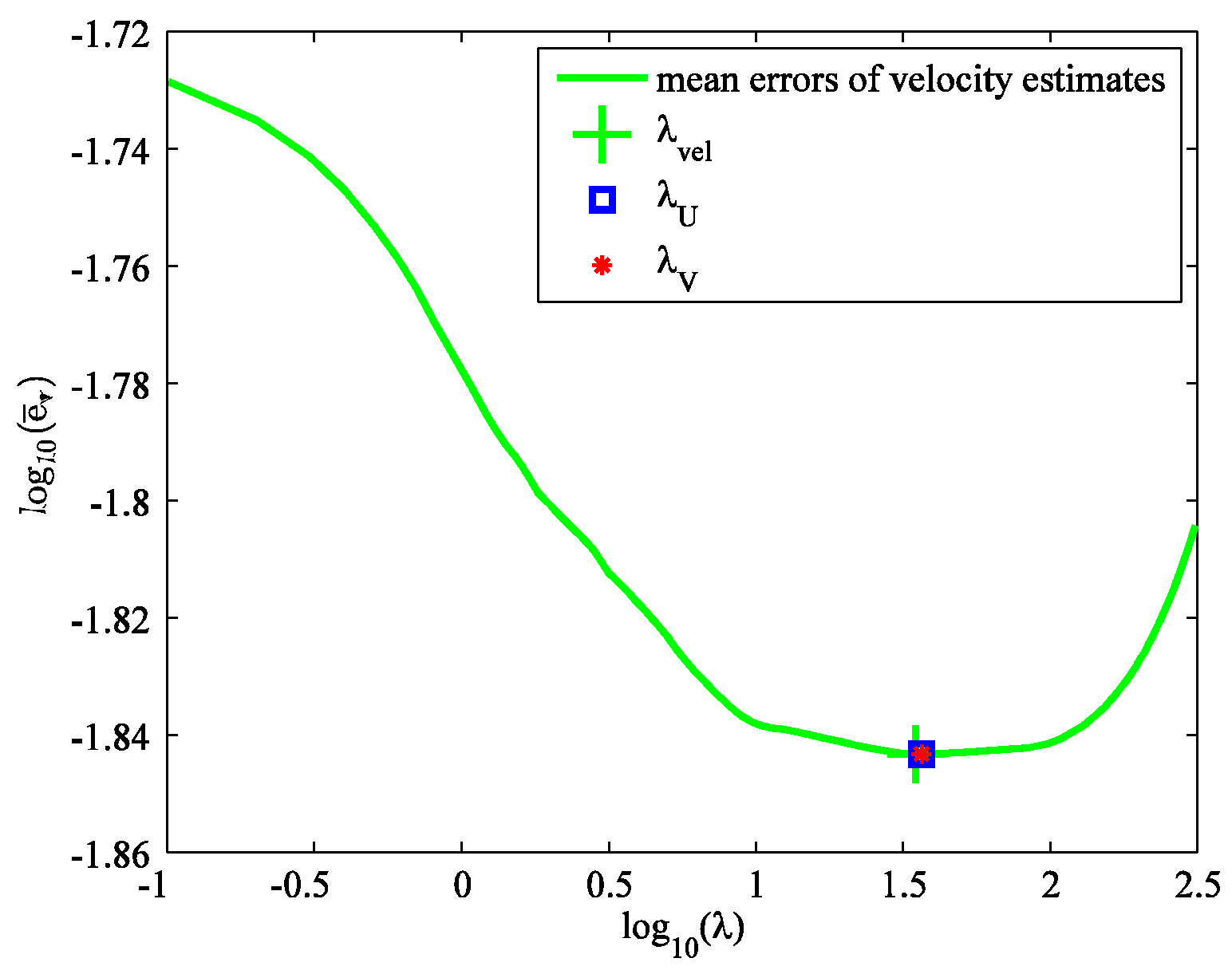
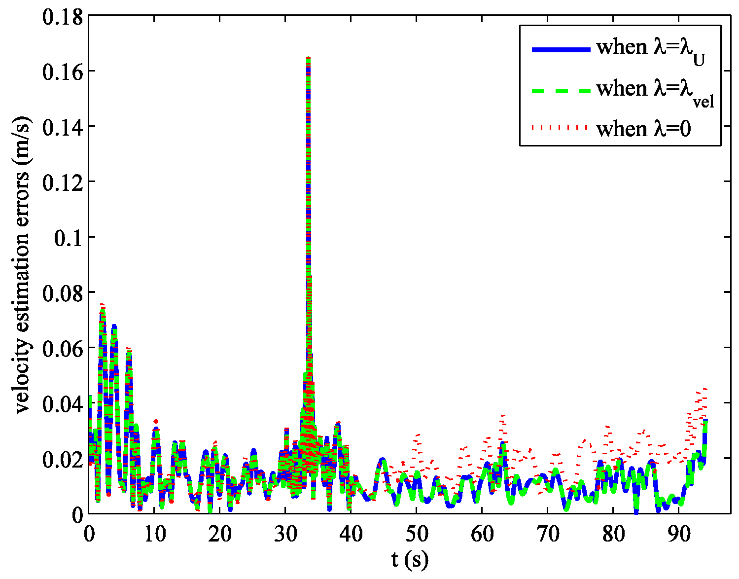
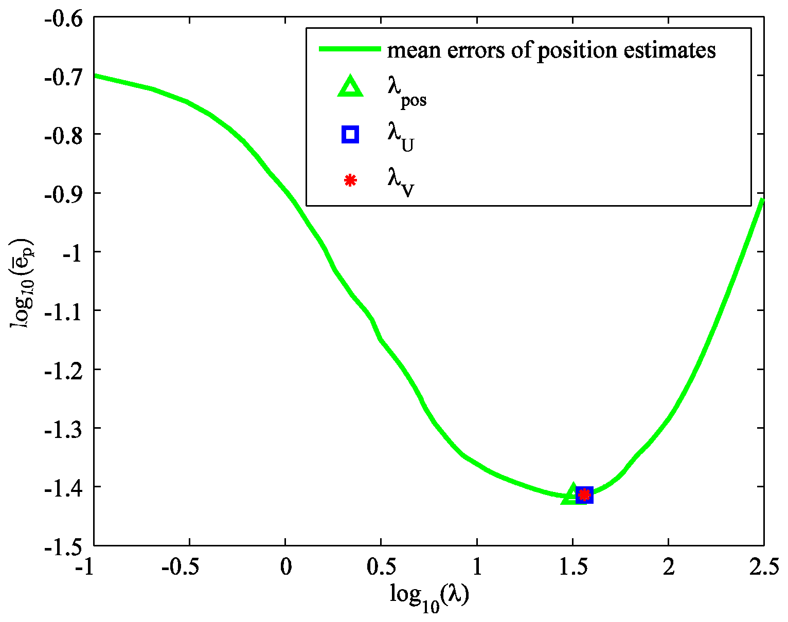
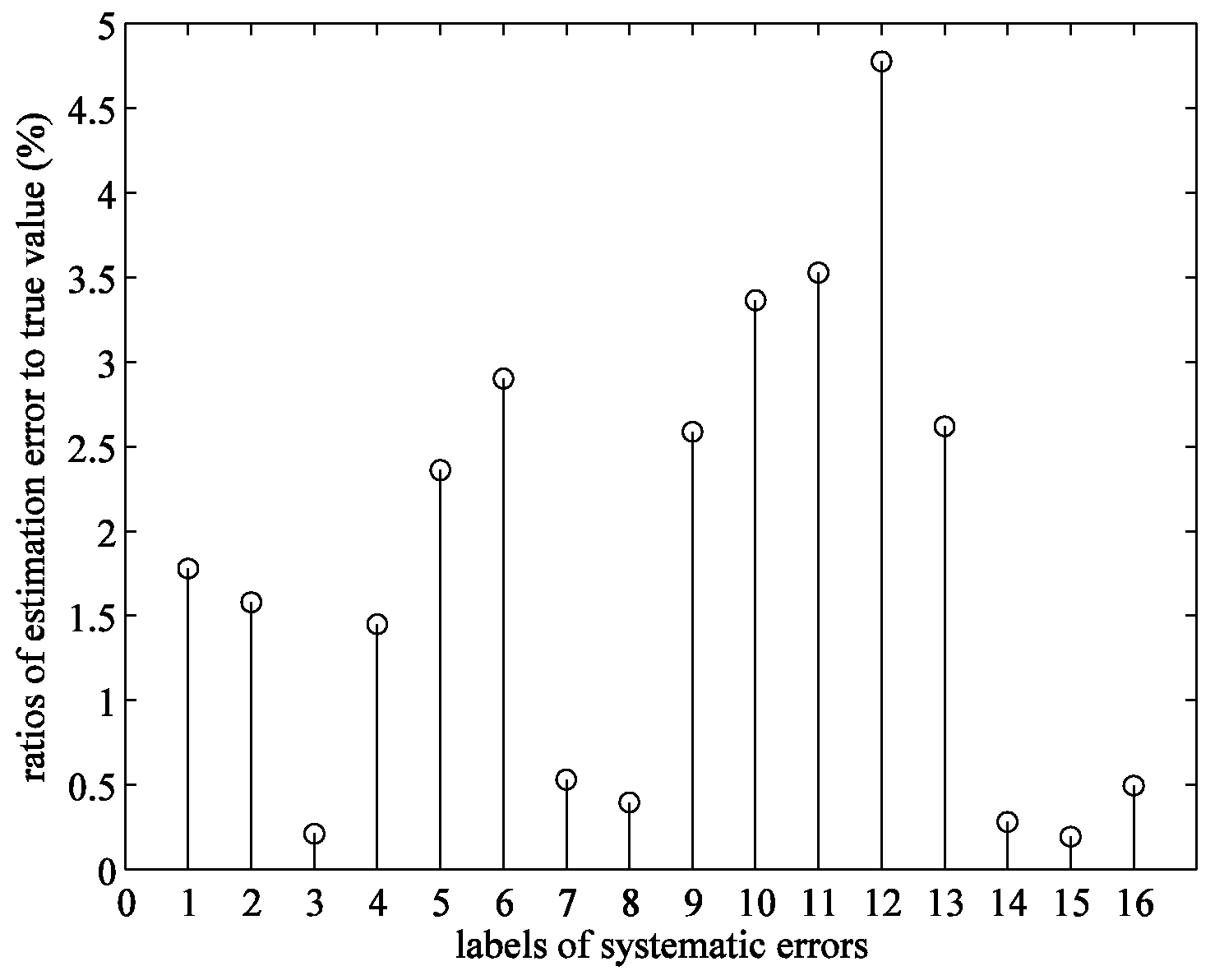
4. Simulation Example

This section presents a tracking scenario of a boost phase ballistic target to demonstrate the performance of our method. The true trajectory with a period of 94 s is generated by the integral of the dynamics equations from [26]. The target has a staging event at about 33.4 s. There are twenty-seven radars and twelve telescope relays tracking the target. At any time, nine radars and four telescopes measure the trajectory simultaneously. The types of radar measurement are range and range-rate, and for optical sensors are azimuth and elevation. The standard deviations for the noise of range and range-rate are 8.3 m and 0.05 m/s, respectively, and the azimuth and elevation noise has the same standard deviation 5″. The systematic errors of measurements are all constant. Three radars have the systematic errors 20 m and 0.2 m/s for the range and range-rate, respectively, three radars have the systematic errors −15 m and −0.1 m/s, and one radar has systematic errors 25 m and 0.3 m/s. One telescope has the systematic errors −30″ and 30″ for the azimuth and elevation, respectively. The left measurements have no systematic errors. Thus, the number of systematic errors to be estimated is sixteen. We use the B-spline of order four to represent the trajectory. This spline can fit the ballistic trajectory very well and is widely used in the literature [2,3,4,5]. The spline knots are selected by using the knots insertion approach in [11], and the number of the B-spline coefficients θ is 344 which is determined by the number of the selected knots. Here, we consider the sparse regularization with p = 1.
Figure 1 shows the SURE U(λ) and the GCV minus σ2 (denoted by V(λ) − σ2) versus the regularization parameter λ in the logarithmic scale. It can be seen that the U(λ) and V(λ) curves have quite similar shapes. The minimizers of U(λ) and V(λ) are λU = 36.1620 and λV = 36.1581, respectively. They are quite close. Figure 2 shows the predictive MSE R(λ) versus λ in the logarithmic scale. We can see that the curve trend is consistent with SURE and GCV. The minimizer is λR = 31.0215, and it is close to λU and λV, indicating that both SURE and GCV methods can give good parameter choices for minimizing the predictive error.
However, we aim at choosing the suitable parameter to minimize the errors of trajectory estimation not the predictive error of measurements. The performance of the trajectory estimation obtained by SURE and GCV approaches should be examined. Given the true trajectory ( x ( t ) , y ( t ) , z ( t ) , x ˙ ( t ) , y ˙ ( t ) , z ˙ ( t ) ) and the estimated trajectory ( x ^ ( t ) , y ^ ( t ) , z ^ ( t ) , x ˙ ^ ( t ) , y ˙ ^ ( t ) , z ˙ ^ ( t ) ) at time t, the errors of position and velocity estimates are defined as
e p ( t ) = ( x ^ ( t ) x ( t ) ) 2 + ( y ^ ( t ) y ( t ) ) 2 + ( z ^ ( t ) z ( t ) ) 2  
e v ( t ) = ( x ˙ ^ ( t ) x ˙ ( t ) ) 2 + ( y ˙ ^ ( t ) y ˙ ( t ) ) 2 + ( z ˙ ^ ( t ) z ˙ ( t ) ) 2  
The mean errors of position and velocity estimates for the entire sampling moments t 1 , t 2 , , t M are defined as e ¯ p = i = 1 M e p ( t i ) / M and e ¯ v = i = 1 M e v ( t i ) / M .
Figure 3 shows the mean errors of position estimates versus λ in the logarithmic scale. The minimizer is λpos = 31.6718. It is close to the minimizers of SURE and GCV. Figure 4 shows the errors of position estimates versus time when λ is set to λU, λpos, and 0. Λ = 0 means that all the potential systematic errors are estimated without sparse regularization. It can be seen that the errors of position estimates for λ = λU and λ = λpos are very close, and much smaller than that of λ = 0. λU and λV are so close that the error curves corresponding to λU and λV are coincident. Thus, we did not plot the curve for λ = λV in Figure 4. The mean errors of position estimates are 0.0387 m, 0.0387 m, 0.0384 m, and 0.2102 m for λ = λU, λV, λpos, and 0, respectively.
For the errors of velocity estimates, we have similar results as with position. The mean errors of velocity estimates versus λ in the logarithmic scale are shown in Figure 5. The unique minimizer of this curve is at λvel = 34.7334. It is also close to the minimizers of SURE and GCV. The errors of velocity estimates versus time when λ = λU, λvel, and 0 are shown in Figure 6. The errors of velocity estimates for λ = λU and λ = λvel are very close, and smaller than that of λ = 0. The mean errors of velocity estimates are 0.01435 m/s, 0.01435 m/s, 0.01435 m/s, and 0.01898 m/s for λ = λU, λV, λvel, and 0, respectively.
The above results suggest that both SURE and GCV methods can provide good parameter choices for minimizing the errors of trajectory estimation, and that our method can improve the precision of trajectory estimation over the traditional RPM method without regularization.
The ratio of estimation error to true value for each item of the systematic errors is defined by | δ ^ δ | / | δ | , where δ ^ and δ are the true value and the estimate for systematic error. Figure 7 shows the ratios of all the systematic errors when λ is set to λU. The maximum ratio is 4.78%, suggesting that our method can achieve the accurate estimates of systematic errors.

5. Conclusions

The key contribution of this paper is a sparse regularization based sensor alignment method involving the selection of a regularization parameter for ballistic trajectory estimation. The sparse regularization model, which combines the traditional model of trajectory estimation with the sparse constraint of the systematic errors, is established. By using the Newton algorithm, the regularization model is solved to obtain the estimates of the trajectory and the systematic errors simultaneously. The SURE and GCV are constructed to select the suitable regularization parameter for optimizing the estimation performance. The computation method for SURE and GCV are also studied. The major improvement for SURE and GCV is that they can manage the nonlinearity of the measurement model. Simulation results show that both SURE and GCV methods can provide the regularization parameter nearly minimizing the error of the trajectory estimates, and that our method outperforms the traditional non-regularization method in terms of the estimation accuracy. The accurate estimates of systematic errors are achieved.

Author Contributions

Conceptualization, D.L.; investigation, D.L.; methodology, D.L. and L.G.; software, L.G.; validation, D.L.; formal analysis, D.L.; visualization, L.G.; writing—original draft preparation, D.L.; writing—review and editing, L.G.; funding acquisition, L.G.

Funding

This research was funded by the National Natural Science Foundation of China (No. 61703408 and 61801482).

Conflicts of Interest

The authors declare no conflict of interest.

References

  1. Wu, Y.; Zhu, J. A fusion method for estimate of trajectory. J. Sci. China Ser. E-Technol. Sci. 1999, 42, 150–156. [Google Scholar] [CrossRef]
  2. Wang, Z.; Zhu, J. Reduced parameter model on trajectory tracking data with applications. J. Sci. China Ser. E-Technol. Sci. 1999, 42, 190–199. [Google Scholar] [CrossRef]
  3. Zhu, J. Data fusion techniques for incomplete measurement of trajectory. Chin. Sci. Bull. 2001, 46, 627–629. [Google Scholar] [CrossRef]
  4. Wang, Z.; Yi, D.; Duan, X.; Yao, J.; Gu, D. Measurement Data Modeling and Parameter Estimation; CRC Press: Boca Raton, FL, USA, 2011; ISBN 978-1-4398-5378-8. [Google Scholar]
  5. Guo, J.; Zhao, H. Accurate algorithm for trajectory determination of launch vehicle in ascent phase. J. Astronautics 2015, 36, 1018–1023. [Google Scholar] [CrossRef]
  6. Zhang, Y.; Ye, W.Z.; Zhang, J.J. Sparse signal recovery by accelerated lq (0 <q <1) thresholding algorithm. Int. J. Comput. Math. 2017, 94, 2481–2491. [Google Scholar] [CrossRef]
  7. Shah, J.; Qureshi, I.; Deng, Y.; Kadir, K. Reconstruction of sparse signals and compressively sampled images based on smooth l1-norm approximation. J. Signal Process. Syst. 2017, 88, 333–344. [Google Scholar] [CrossRef]
  8. Bevacqua, M.T.; Isernia, T. Shape reconstruction via equivalence principle, constrained inverse source problems and sparsity promotion. Prog. Electromagn. Res. 2017, 158, 37–48. [Google Scholar] [CrossRef]
  9. Sun, S.; Kooij, B.J.; Yarovoy, A.G. Linearized 3-D electromagnetic contrast source inversion and its applications to half-space configurations. IEEE Trans. Geosci. Remote Sens. 2017, 55, 3475–3487. [Google Scholar] [CrossRef]
  10. Bevacqua, M.T.; Isernia, T. A boundary indicator for aspect limited sensing of hidden dielectric objects. IEEE Geosci. Remote Sens. Lett. 2018, 15, 838–842. [Google Scholar] [CrossRef]
  11. Liu, J.; Zhu, J.; Xie, M. Trajectory estimation with multi-range-rate system based on sparse representation and spline model optimization. Chin. J. Aeronaut. 2010, 23, 84–90. [Google Scholar] [CrossRef]
  12. Hansen, P.C. Analysis of discrete ill-posed problems by means of the L-curve. SIAM Rev. 1992, 34, 561–580. [Google Scholar] [CrossRef]
  13. Reginska, T. A regularization parameter in discrete ill-posed problem. SIAM J. Sci. Comput. 1996, 17, 740–749. [Google Scholar] [CrossRef]
  14. Batu, O.; Cetin, M. Parameter selection in sparsity-driven SAR imaging. IEEE Trans. Aerosp. Electr. Syst. 2011, 47, 3040–3050. [Google Scholar] [CrossRef]
  15. Ramani, S.; Blu, T.; Unser, M. Monte-carlo sure: A black-box optimization of regularization parameters for general denoising algorithms. IEEE Trans. Image Proc. 2008, 17, 1540–1554. [Google Scholar] [CrossRef] [PubMed]
  16. Ramani, S.; Liu, Z.; Rosen, J.; Nielsen, J.-F.; Fessler, J.A. Regularization parameter selection for nonlinear iterative image restoration and MRI reconstruction using GCV and SURE based methods. IEEE Trans. Image Proc. 2012, 21, 3659–3672. [Google Scholar] [CrossRef] [PubMed]
  17. Xue, F.; Yagola, A.G.; Liu, J.; Meng, G. Recursive SURE for iterative reweighted least square algorithms. Inverse Probl. Sci. Eng. 2016, 24, 625–646. [Google Scholar] [CrossRef]
  18. Craven, P.; Wahba, G. Smoothing noisy data with spline functions. Numer. Math. 1979, 31, 377–403. [Google Scholar] [CrossRef]
  19. Jansen, M. Generalized cross validation in variable selection with and without shrinkage. J. Stat. Plan. Inf. 2015, 159, 90–104. [Google Scholar] [CrossRef]
  20. Fenu, C.; Reichel, L.; Rodriguez, G. GCV for Tikhonov regularization via global Golub-Kahan decomposition. Numer. Linear Algebra Appl. 2016, 23, 467–484. [Google Scholar] [CrossRef]
  21. Hanke, M. Limitations of the L-curve method in ill-posed problem. BIT Numer. Math. 1996, 36, 287–301. [Google Scholar] [CrossRef]
  22. Vogel, C.R. Computational Methods for Inverse Problems; SIAM: Philadelphia, PA, USA, 2002; ISBN 0-89871-507-5. [Google Scholar]
  23. Li, X.R.; Jilkov, V.P. Survey of maneuvering target tracking. PartII: Motion models of ballistic and space targets. IEEE Trans. Aerosp. Elec. Sys. 2010, 46, 96–119. [Google Scholar] [CrossRef]
  24. Kelley, C.T. Iterative Methods for Optimization; SIAM: Philadelphia, PA, USA, 1995. [Google Scholar]
  25. Stein, C.M. Estimation of the mean of a multivariate normal distribution. Ann. Stat. 1981, 9, 1135–1151. [Google Scholar] [CrossRef]
  26. Hough, M.E. Nonlinear recursive filter for boost trajectories. J. Guid. Control Dyn. 2001, 24, 991–997. [Google Scholar] [CrossRef]
Figure 1. Stein’s unbiased risk estimator (SURE) and general cross-validation (GCV)-σ2 versus λ in logarithmic scale.
Information 09 00255 g001
Figure 2. Predictive mean square error (MSE) versus λ in logarithmic scale.
Information 09 00255 g002
Figure 3. Mean errors of position estimates versus λ in logarithmic scale.
Information 09 00255 g003
Figure 4. Errors of position estimates versus time when λ = λU, λpos, and 0.
Information 09 00255 g004
Figure 5. Mean errors of velocity estimates versus λ in logarithmic scale.
Information 09 00255 g005
Figure 6. Errors of velocity estimates versus time when λ = λU, λvel, and 0.
Information 09 00255 g006
Figure 7. Ratios of estimation error to true value for systematic errors when λ=λU.
Information 09 00255 g007

