Article

Decentralized State-Observer-Based Traffic Density Estimation of Large-Scale Urban Freeway Network by Dynamic Model

1
College of Metropolitan Transportation, Beijing University of Technology, Beijing 100124, China
2
Beijing Key Laboratory of Transportation Engineering, Beijing 100124, China
3
Beijing Collaborative Innovation Center for Metropolitan Transportation, Beijing 100124, China
*
Author to whom correspondence should be addressed.
Information 2017, 8(3), 95; https://doi.org/10.3390/info8030095
Submission received: 27 June 2017 / Revised: 24 July 2017 / Accepted: 31 July 2017 / Published: 3 August 2017

Abstract

:
In order to estimate traffic densities in a large-scale urban freeway network in an accurate and timely fashion when traffic sensors do not cover the freeway network completely and thus only local measurement data can be utilized, this paper proposes a decentralized state observer approach based on a macroscopic traffic flow model. Firstly, by using the well-known cell transmission model (CTM), the urban freeway network is modeled in the way of distributed systems. Secondly, based on the model, a decentralized observer is designed. With the help of the Lyapunov function and S-procedure theory, the observer gains are computed by using linear matrix inequality (LMI) technique. So, the traffic densities of the whole road network can be estimated by the designed observer. Finally, this method is applied to the outer ring of the Beijing’s second ring road and experimental results demonstrate the effectiveness and applicability of the proposed approach.

1. Introduction

As one of the most important parameters of traffic flow and a key index to identify traffic state, traffic density estimation remains one of the major concerns in urban traffic networks. In recent years, various strategies have been proposed for tackling related problems in traffic density estimation. Most of these methods are based on the use of a macroscopic traffic flow model, since Daganzo proposed the well-known cell transmission model (CTM) [1,2]. Muñoz and Sun et al. presented the switching mode model (SMM) based on the CTM which is well suited for model-based traffic density estimation [3], and they further applied a semi-automated method to the California Freeway [4]. Nevertheless, this approach has two major drawbacks. Firstly, it requires an accurate road network model and a precise initial state; if the two key points cannot be met, it will result in an unacceptable estimated error. Secondly, the model itself is not robust, so once the traffic network is disturbed by noise, the estimated results are still inaccurate. Therefore, other approaches were studied based on the dynamic model, as the efficient practical tools, based-model state observer and Kalman filter were utilized in traffic state estimation. Alvarez-Icaza et al. [5] adopted the adaptive observer to estimate vehicle densities. Canudas-de-Wit et al. [6] proposed the graph constrained-CTM observer and applied it to reconstruct the densities of the Grenoble south ring, and in [7] they further introduced a robust mode selector for the uncertain graph constrained switching mode model and applied it to highway traffic densities estimation via a switched state observer. Chen and Guo et al. [8,9] deduced a piecewise affine linear system (PWALS) by combining the cell transmission model (CTM) with the dynamic graph hybrid automata (DGHA), and then based on the model designed switched state observer to estimate traffic densities. In addition, Wang and Papageorgiou [10] proposed a general stochastic macroscopic traffic flow model of freeway stretches, and based on this model the extended Kalman filter was designed to estimate traffic state in freeway stretches. Juan and Alexandre [11] presented a new algorithm to integrate GPS data in flow models, and compared it to an application of Kalman filtering for the specific problem of interest.
However, the high computational complexity and intolerable delay limit those centralized observers mentioned above cannot be effectively applied to large-scale road networks. Consequently, we must consider another estimated strategy. To the best of our knowledge, decentralized estimation algorithm is a practical tool to solve the estimation problem of the large-scale system, and a larger amount of literature is available on decentralized observer for state estimation. In reference [12,13], a decentralized state observer was presented to solve the state estimation problem for a class of norm-bounded nonlinear systems. In reference [14,15,16], decentralized observers were applied to large-scale continuous interconnected systems. Unfortunately, although such methods were widely adopted in different large-scale systems, they cannot be applied directly in our urban freeway network because they were based on a continuous system.
In this paper, our goal is to design a decentralized state observer based on the dynamic model to estimate traffic densities for a large-scale urban freeway network. By introducing the S-procedure and the Lyapunov function approach for the estimation error system, the corresponding observer gain matrices can be computed. This is also one of the most significant contributions of this paper.
On the other hand, it is important to note that the observability problem on the traffic network setting is the pre-step of the estimation problem. Unless establishing that the road network system is observable, estimation problem should not be approached. This problem is closely related to the traffic sensors placement in the road network. Contreras et al. [17] proposed a solution to the observability problem in a dynamical setting on a straight road segment. Agarwal et al. [18] extended the methodology to complex traffic networks using the complex modeling framework proposed in reference [19]. Contreras et al. [20] further explored the quality of traffic observability and state estimation on Highways in a Lagrangian setting.
The rest of the paper is organized as follows. In Section 2, we provide some relevant background material and state the problem. In Section 3, the decentralized state observer is designed based on the urban freeway network model. In Section 4, we illustrate the obtained results by applying them to the outer ring of Beijing’s second ring road. The paper is concluded in Section 5.

2. Preliminaries and Problem Formula

The macroscopic traffic flow model of an urban freeway network has been proposed by combining the dynamic graph hybrid automata (DGHA) with the cell transmission model (CTM), and as a result, the traffic flow network can be deduced a centralized piecewise affine linear system (PWALS) in our previous work [9]. The detailed modeling process can be seen in reference [9].
x t + 1 = A σ t x t + B σ ( t ) u ( t ) + F σ t y t = C x t
where x = [ ρ 1 , , ρ n ] T R n denotes the traffic density vector of the road network, the input vector u R m is added to the traffic demand of the road network, y ( t ) R p is the measured output vector of the traffic sensors, A σ and B σ are the system matrix and input matrix, respectively. C is the output matrix depending on the type number and location of the sensors. F σ is a vector consisting of the parameters in the fundamental diagrams of all the road segments. σ : [ 0 , + ) { 1 , 2 , , k } is the switching function that maps the index time stage into an index set { 1 , 2 , , k } , and each of the indices corresponds to a different mode of the system.
In the model, the triangular fundamental diagram (Figure 1) is used to approximately describe the relationship between traffic flow and density of road segment (cell), where ρ i is the traffic density (vpkm), q i is the traffic flow (vph), C i is the traffic capacity (vph), V i is the free flow speed (kmph), W i is the traffic wave speed (kmph), ρ i 0 is the critical density (vpkm), and ρ i m is the maximum/jam density (vpkm).
In reference [9], based on model (1), the following centralized state observer was designed to estimate the traffic densities:
x ^ t + 1 = A σ t x ^ t + B σ t u t + F σ t + K σ t y t C x ^ t y ^ t = C x ^ t
where x ^ t R n denotes the estimated density vector, y ^ t R p is the output vector of the observer, and K σ is the gain matrix of the observer.
The estimation error dynamic system can be obtained by combining Equation (1) with Equation (2):
e t + 1 = A σ t K σ t C e t
For the system (1), if the pair ( A σ , C ) is observable or detectable, then the matrix K σ can be designed so that the matrix A σ t K σ t C is Hurwitz and the e ( t ) is convergent with time.
However, the state observer (2) is inherently centralized, and it cannot be applied effectively in a large-scale freeway network for the following reasons:
(i) The estimated state x ^ ( t ) is of high dimension, causing complicated computational effort and intolerable delay; (ii) Local problems will cause paralysis of the entire dynamic network system because of its centralized structure; (iii) The requirement of global information communication; (iv) Real-time continuous communication of all measurements to a central processor is required.
Consequently, this paper proposes a decentralized observer design strategy to solve the estimated problem of a large-scale urban freeway network.

3. Decentralized State Observer Design

To the best of our knowledge, the decentralized state observer is an effective practical tool and can fill in the gap of density estimation for large-scale freeway networks. In this paper, we only consider the situation of fixed mode (without switching case). We assume that an urban freeway can be divided into N sections, that each one can be seen a subsystem, and the dynamics of the i-th one is described as follows:
x i t + 1 = A i x i t + B i u i t + j N i A i j x j t + F i y i t = C i x i t , i = 1 , , N
where x i R n i is the traffic density vector of the subsystem i, x j R n j is the density vector of all the neighbors of subsystem i, the input vector u i R m i is added to represent the traffic demand of the subsystem i, y i R p i is the measured output vector of the sensors in subsystem i, and A i , B i , and C i are the system matrix, the input matrix, and the output matrix with appropriate dimension, respectively. F i is the affine item. N i = N i in + N i out , N i in = j 1 , , N \ i : A i j σ t 0 denotes the in-neighbors of subsystem i, and N i out = j 1 , , N \ i : A j i σ t 0 denotes the out-neighbors of subsystem i.
Here we denote h i t , x = j N i A i j x j t .
So, Equation (4) can be written as follows:
x i t + 1 = A i x i t + B i u i t + F i + h i t , x y i t = C i x i t
where the h i t , x denotes the interconnected terms illustrating the nonlinearity of the i-th subsystem.
The compact form of the overall system can then be written as follows:
x t + 1 = A x t + B u t + F + h t , x y t = C x t
where x = [ ρ 1 T , , ρ N T ] T , u = [ u 1 T , , u N T ] T and y = [ y 1 T , , y N T ] T are the state vector, the input vector and the measured output vector of the global system, respectively. h t , x = h = h 1 T , h 2 T , h N T is the interconnected term between the adjacent subsystem. A = d i a g A i , B = d i a g B i , C = d i a g C i , F = d i a g F i .
The interconnected term h t , x satisfies the following quadratic inequality
h T t , x h t , x λ 2 x T H T H x
where λ is positive constant and H is a constant matrix.
The state observer of subsystem i is as follows:
x ^ i t + 1 = A i x ^ i t + B i u i t + F i + K i y i t y ^ i t y ^ i t = C i x ^ i t , i = 1 , , N
where K i is the local observer gain matrix to be designed in the following.
The observer of the global system can be designed in the following form:
x ^ t + 1 = A x ^ t + B u t + F + K y t y ^ t y ^ t = C x ^ t
where x ^ T = x ^ 1 T , , x ^ N T is the estimated traffic density vector, y ^ is the observer output vector, and K = blkdig K 1 , , K N is the observer gain matrix to be computed in the following.
The error dynamics between the real state and the estimated one, e = x x ^ , can be described by the following difference equation
e t + 1 = A K C e t + h t , x
As we all know, in order to reconstruct the actual traffic densities of a road network by using the designed state observer, the error dynamic system e ( t + 1 ) must be convergent. On the other hand, if the pair ( A , C ) is observable or detectable, we can find a gain matrix K such that the matrix A K C is Hurwitz. However, the stability of the error system (10) cannot be guaranteed, due to the existence of the interconnected item h ( t , x ) . We can solve the problem for the large-scale interconnected systems by employing the S-procedure approach [21], and thus the decentralized observer design is transformed into the feasible solution of the linear matrix inequality (LMI). Eventually, the observer gain can be computed by using the LMI technique [22].
First of all, for (10) to be asymptotically stable, a Lyapunov function V ( e ) = e T P e should exist such that Δ V ( e ) < 0 . So, the following Inequality (11) is satisfied:
Δ V ( e ) = V e ( t + 1 ) V e ( t ) = [ ( A K C ) e + h ] T P [ ( A K C ) e + h ] e T P e = e T A K C T P A K C P e + e T A K C T P h + h T P A K C e + h T P h < 0
where P is a symmetric positive definite matrix.
Furthermore, we can obtain a constraint from Inequality (7):
λ 2 x H T H x h T t , x h t , x 0
Next, by introducing S-procedure and combining (11) with (12), there must exist a nonnegative constant μ so that the Inequality (13) is satisfied:
e T A K C T P A K C P e + e T A K C T P h + h T P A K C e + h T P h + μ λ 2 x H T H x h T t , x h t , x < 0
Therefore, Equation (13) can be written as follows:
x T e T h T μ λ 2 H T H 0 0 0 W A K C T P 0 P A K C P μ I x e h < 0
Namely:
μ λ 2 H T H 0 0 0 W A K C T P 0 P A K C P μ I < 0
where W = A K C T P A K C P .
Notice that the Inequality (15) is not a linear matrix inequality because it contains the bilinearities, but can be made so by employing the change of variable, where G = P K , Q = K G . The transformed problem is now of LMI variety. Eventually, the observer gain matrix can be calculated by K = P 1 G .
Remark 1.
The stability of the error system (10) can be transformed into the feasible solution of the linear matrix inequality (LMI) (15); thus, if a feasible solution of (15) exists, then the stability of the error system (10) is guaranteed.

4. Experimental Results and Analysis

4.1. Data Collection and Parameter Settings

In this section, we will take the outer ring of Beijing’s second ring road (Figure 2) as an application to verify the performance of the proposed approach. The outer ring is approximately 33 km long and includes 37 on-ramps and 53 off-ramps. According to the homogeneous rule of cell division [8], the outer ring freeway can be divided into 100 cells, and the whole road network was partitioned into 4 sections. Each one can be seen as one subsystem which contains 25 cells, and the cell lengths are listed in Appendix A.
The first step for preparing the experiment was the development of a microscopic model for the outer ring road using the traffic simulator VISSIM. After achieving the correct freeway architecture, we proceeded with the identification of the macroscopic characteristics (e.g., split ratio and demand flows) necessary to tune the whole microscopic simulator. Additionally, we obtained the real traffic state of the outer ring (on 10 December 2016) from the Beijing Collaborative Innovation Center for Metropolitan Transportation. Therefore, by using the road network model of the outer ring road built by VISSIM, we further mimicked the traffic flow evolution from about 22:00 p.m. to 04:00 a.m.
Moreover, according to the difference of turning radius, we classed the roads (cells) into the various curves which are marked in blue boxes in Figure 2, and further fitted the flow-density relationship of road segments with an off-line identification process by using a least square approximation approach with the help of the VISSIM simulator and obtained the fundamental parameters; the results are listed in Table 1.
The corresponding matrices A s = [ a i , j ] and B s = [ b i , j ] , s = 1 , 2 , 3 , 4 , are listed in Appendix B. Here the sample time period T = 5 s such that the condition V i T L i , i = 1 , 2 100 , is satisfied.

4.2. Traffic Sensor Placement

As the pre-step of estimation problem, the observability problem is closely related with the study of the traffic sensor placement problem. The observability problem of a given network determines how many, where, and what types of sensors would be required to completely estimate all the states of the given road network system. Hence, it is extremely essential to analyze the observability problem in traffic networks.
The measurement output matrix C in Equation (6) is used to identify different sensor placements. We will use this to analyze the observability problem on the outer ring of Beijing’s second ring freeway. To the best of our knowledge, different types of sensor technologies can be applied widely to collect traffic data, including floating vehicle, loop detector, microwave, video, etc. Different source data can provide different measurement outputs, and thus one gets different types of matrix C in the measurement output equation. One can even utilize the fused data or multi-dimensional data of several types of sensors at the same time.
In this paper, to ensure that each subsystem is observable, the virtual loop detectors in VISSIM installed in cells 1, 3, 5, 7, 11, 13, 15, 20, 23, and 25 were used to collect traffic densities. Hence, corresponding to these detectors, c s i , j , s = 1 , 2 , 3 , 4 is a 10 × 25 matrix with entries c s 1 , 1 = c s 2 , 3 = c s 3 , 5 = c s 4 , 7 = c s 5 , 11 = c s 6 , 13 = c s 7 , 15 = c s 8 , 20 = c s 9 , 23 = c s 10 , 25 = 1 and c s i , j = 0 for the other i , j . Moreover, one can verify that the pair ( A s , C s ) is observable for all s = 1 , 2 , 3 , 4 by calculating the observability matrix.
Meanwhile, we collect traffic densities by using loop detectors which are set in each cell (validation purposes) of Beijing’s second ring freeway built by VISSIM mentioned above, and we call these densities the simulated ones.

4.3. Analysis of Results

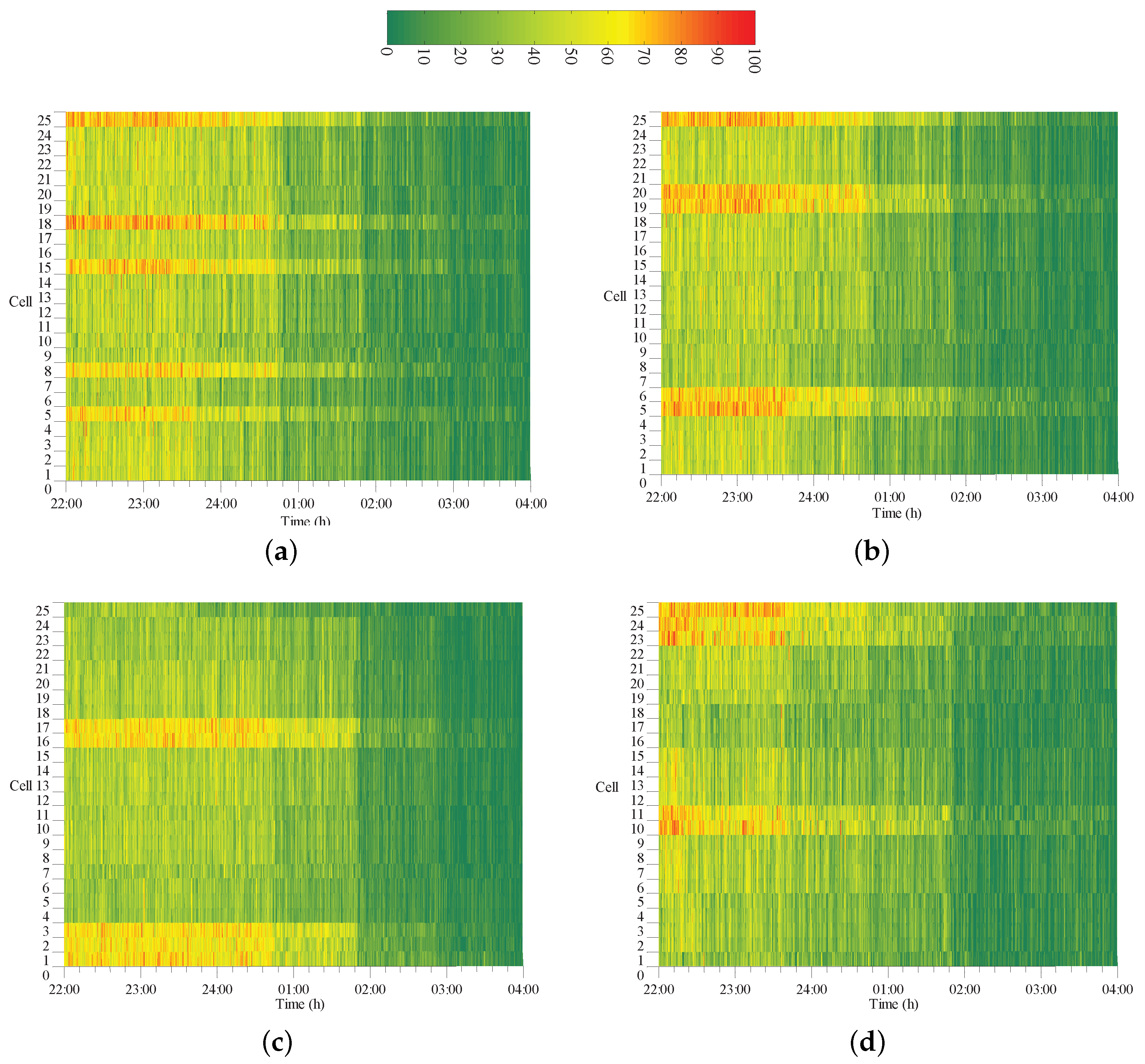
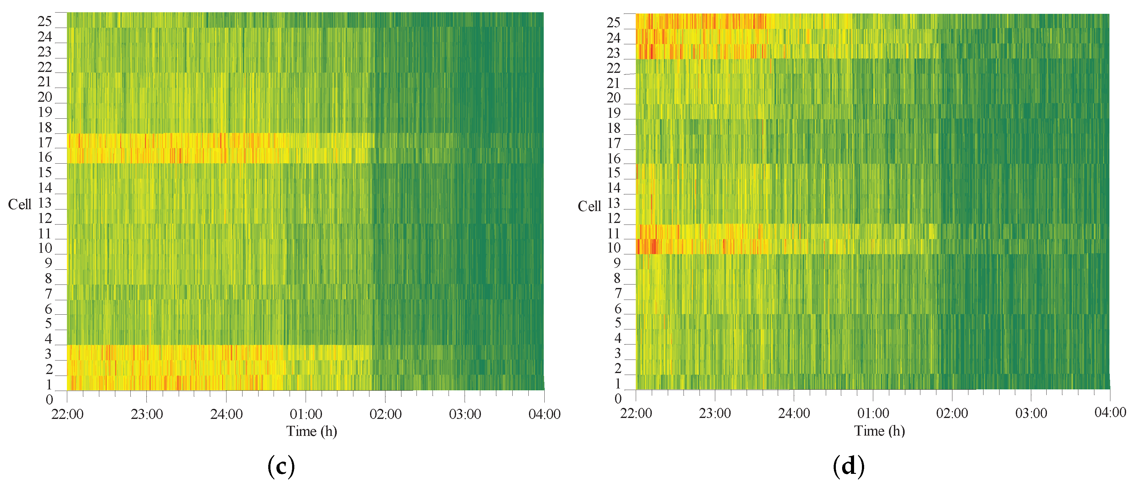
The experimental results for the outer ring freeway are shown in Figure 3 and Figure 4 in the form of time-space diagrams, where Figure 3 is the simulated densities from 22:00 p.m. to 04:00 a.m. and Figure 4 presents the estimated densities obtained by the designed observer. It is clear that the densities of all road segments are smaller than the critical ones after about 22:00, and the traffic flows gradually decreased with time. Especially, there are almost no vehicles on the road after about 24:00.
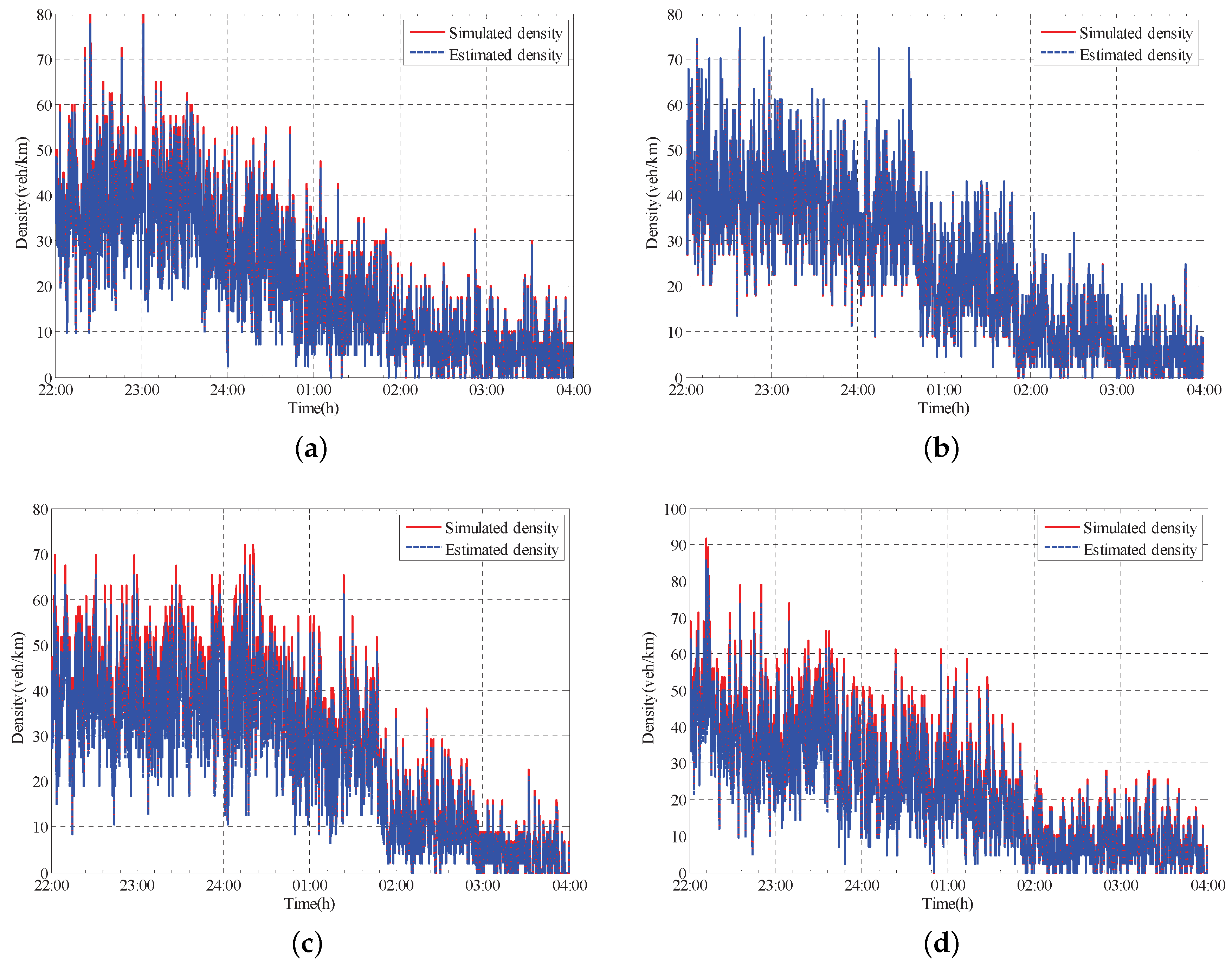
In order to further demonstrate the estimated effect of the observer, cells 6, 41, 70, and 88 are presented to exhibit the density comparison in more detail (see Figure 5). From Figure 4 and Figure 5, we can see that the decentralized observer is feasible, and the estimated densities can approximate the simulated ones.
The performance indicator of the state observer is given by using the mean square error (MSE), which is defined by Equation (16); Table 2 shows the mean value of MSE for each subsystem.
MSE = i = 1 n ρ ^ i ρ i 2 n
From Table 2, we can further calculate that the mean value of the overall freeway network is approximately 13.115 % . The results indicate that the designed decentralized state observer has a good estimated performance.

5. Conclusions and Future Work

In this paper, based on the macroscopic traffic flow model, we have designed a decentralized state observer to estimate the traffic densities of a large-scale urban freeway network. The LMI techniques and S-procedure method were both used to compute the observer gain matrices. Moreover, experimental results of the outer ring of Beijing’s second ring freeway exhibited the estimated densities, and the simulated densities obtained from the VISSIM traffic simulator agree closely. We have shown that the traffic densities of the road segments not equipped with sensors can be reconstructed by using the designed observer.
However, it should be noted that the developed urban freeway network model and the simulated data in this paper have some limitations which need to be improved upon in future research.
Firstly, we only considered the fixed mode case; so, in future research, the switched-type traffic model and decentralized observer are both required. Secondly, in the application example, we only used the simulation data obtained by VISSIM to justify the performance of the designed observer; in future research, we need to collect real traffic data for the practical application to further verify our proposed approach.

Acknowledgments

The work was supported by the National Natural Science Foundation of China (Grant No. 61573030).

Author Contributions

Yangzhou Chen modeled the urban freeway network; Yangzhou Chen and Yuqi Guo conceived and designed the experiments; Yuqi Guo and Chiyuan Zhang performed the experiments and analyzed the data; Yangzhou Chen and Yuqi Guo wrote the paper.

Conflicts of Interest

The authors declare no conflict of interest.

Appendix A

Table A1. Cell length of Beijing’s second ring road.
NumberLengthNumberLengthNumberLengthNumberLength
1215 m26661 m51318 m76133 m
2700 m27112 m52232 m77337 m
3170 m28726 m53260 m78368 m
4382 m29607 m54185 m79158 m
5182 m30356 m55185 m80330 m
6456 m31445 m56270 m81358 m
7423 m32445 m57296 m82283 m
8288 m33406 m58301 m83347 m
9370 m34277 m59336 m84306 m
10204 m35505 m60160 m85391 m
11339 m36467 m61136 m86288 m
12132 m37477 m62108 m87370 m
13240 m38160 m63100 m88305 m
14450 m39418 m6496 m89125 m
15236 m40421 m65265 m90651 m
16123 m41415 m66135 m91127 m
17753 m42130 m67185 m92426 m
18508 m43270 m68393 m93146 m
19508 m44336 m69475 m94231 m
20198 m45336 m70363 m95308 m
21608 m46211 m71195 m96421 m
22150 m47290 m72237 m97240 m
23845 m48316 m73396 m98329 m
24278 m49561 m74429 m99317 m
25435 m50411 m75168 m100223 m

Appendix B

Subsystem 1:
A 1 = [ a i , j ] , a 1 , 1 = 0.6123 , a 2 , 1 = 0.1191 , a 2 , 2 = 0.8809 , a 3 , 2 = 0.4903 , a 3 , 3 = 0.5097 , a 4 , 3 = 0.2182 , a 4 , 4 = 0.7818 , a 5 , 4 = 0.4580 , a 5 , 5 = 0.5420 , a 6 , 5 = 0.1828 , a 6 , 6 = 0.8172 , a 7 , 6 = 0.1970 , a 7 , 7 = 0.8030 , a 8 , 7 = 0.2894 , a 8 , 8 = 0.7106 , a 9 , 8 = 0.2253 , a 9 , 9 = 0.7747 , a 10 , 9 = 0.4086 , a 10 , 10 = 0.5914 , a 11 , 10 = 0.2459 , a 11 , 11 = 0.7541 , a 12 , 11 = 0.6314 , a 12 , 12 = 0.3686 , a 13 , 12 = 0.3473 , a 13 , 13 = 0.6527 , a 14 , 13 = 0.1852 , a 14 , 14 = 0.8148 , a 15 , 14 = 0.3532 , a 15 , 15 = 0.6468 , a 16 , 15 = 0.6776 , a 16 , 16 = 0.3224 , a 17 , 16 = 0.1107 , a 17 , 17 = 0.8893 , a 18 , 17 = 0.1641 , a 18 , 18 = 0.8359 , a 19 , 18 = 0.1641 , a 19 , 19 = 0.8359 , a 20 , 19 = 0.4210 , a 20 , 20 = 0.5790 , a 21 , 20 = 0.1371 , a 21 , 21 = 0.8629 , a 22 , 21 = 0.5557 , a 22 , 22 = 0.4443 , a 23 , 22 = 0.0986 , a 23 , 23 = 0.9014 , a 24 , 23 = 0.2998 , a 24 , 24 = 0.7002 , a 25 , 24 = 0.1916 , a 25 , 25 = 0.8084 .
For the subsystem 1 with 12 on-ramps the matrix B 1 = [ b i , j ] is a constant matrix with the entries b 1 , 1 = 0.02326 , b 3 , 2 = 0.02941 , b 5 , 3 = 0.02747 , b 7 , 4 = 0.01748 , b 9 , 5 = 0.01351 , b 11 , 6 = 0.01475 , b 14 , 7 = 0.01111 , b 15 , 8 = 0.02112 , b 17 , 9 = 0.01489 , b 20 , 10 = 0.02525 , b 22 , 11 = 0.0333 , b 25 , 12 = 0.01149 , and b i , j = 0 for the other entries in B 1 .
Subsystem 2:
A 2 = [ a i , j ] , a 1 , 1 = 0.8739 , a 2 , 1 = 0.7442 , a 2 , 2 = 0.2558 , a 3 , 2 = 0.1148 , a 3 , 3 = 0.8852 , a 4 , 3 = 0.1373 , a 4 , 4 = 0.8627 , a 5 , 4 = 0.2341 , a 5 , 5 = 0.7659 , a 6 , 5 = 0.1873 , a 6 , 6 = 0.8127 , a 7 , 6 = 0.1873 , a 7 , 7 = 0.8127 , a 8 , 7 = 0.2053 , a 8 , 8 = 0.7947 , a 9 , 8 = 0.3009 , a 9 , 9 = 0.6991 , a 10 , 9 = 0.1650 , a 10 , 10 = 0.8350 , a 11 , 10 = 0.1785 , a 11 , 11 = 0.8215 , a 12 , 11 = 0.1747 , a 12 , 12 = 0.8253 , a 13 , 12 = 0.5209 , a 13 , 13 = 0.4791 , a 14 , 13 = 0.1994 , a 14 , 14 = 0.8006 , a 15 , 14 = 0.1980 , a 15 , 15 = 0.8020 , a 16 , 15 = 0.2008 , a 16 , 16 = 0.7992 , a 17 , 16 = 0.6412 , a 17 , 17 = 0.3588 , a 18 , 17 = 0.3087 , a 18 , 18 = 0.6913 , a 19 , 18 = 0.2481 , a 19 , 19 = 0.7519 , a 20 , 19 = 0.2481 , a 20 , 20 = 0.7519 , a 21 , 20 = 0.3950 , a 21 , 21 = 0.6050 , a 22 , 21 = 0.2874 , a 22 , 22 = 0.7126 , a 23 , 22 = 0.2638 , a 23 , 23 = 0.7362 , a 24 , 23 = 0.1486 , a 24 , 24 = 0.8514 , a 25 , 24 = 0.2028 , a 25 , 25 = 0.7972 .
For the subsystem 2 with 8 on-ramps the matrix B 2 = [ b i , j ] is a constant matrix with the entries b 2 , 1 = 0.04464 , b 5 , 2 = 0.01404 , b 8 , 3 = 0.01231 , b 11 , 4 = 0.01071 , b 15 , 5 = 0.01188 , b 21 , 6 = 0.02370 , b 23 , 7 = 0.01582 , b 24 , 8 = 0.00891 , and b i , j = 0 for the other entries in B 1 .
Subsystem 3:
A 3 = [ a i , j ] , a 1 , 1 = 0.7379 , a 2 , 1 = 0.3593 , a 2 , 2 = 0.6407 , a 3 , 2 = 0.3206 , a 3 , 3 = 0.6794 , a 4 , 3 = 0.4505 , a 4 , 4 = 0.5495 , a 5 , 4 = 0.4505 , a 5 , 5 = 0.5495 , a 6 , 5 = 0.3087 , a 6 , 6 = 0.6913 , a 7 , 6 = 0.2816 , a 7 , 7 = 0.7184 , a 8 , 7 = 0.2769 , a 8 , 8 = 0.7231 , a 9 , 8 = 0.2481 , a 9 , 9 = 0.7519 , a 10 , 9 = 0.5209 , a 10 , 10 = 0.4791 , a 11 , 10 = 0.6129 , a 11 , 11 = 0.3871 , a 12 , 11 = 0.7718 , a 12 , 12 = 0.2282 , a 13 , 12 = 0.8335 , a 13 , 13 = 0.1665 , a 14 , 13 = 0.8682 , a 14 , 14 = 0.1318 , a 15 , 14 = 0.3145 , a 15 , 15 = 0.6855 , a 16 , 15 = 0.6174 , a 16 , 16 = 0.3826 , a 17 , 16 = 0.4505 , a 17 , 17 = 0.5495 , a 18 , 17 = 0.2121 , a 18 , 18 = 0.7879 , a 19 , 18 = 0.1755 , a 19 , 19 = 0.8245 , a 20 , 19 = 0.2296 , a 20 , 20 = 0.7704 , a 21 , 20 = 0.4274 , a 21 , 21 = 0.5726 , a 22 , 21 = 0.3517 , a 22 , 22 = 0.6483 , a 23 , 22 = 0.2105 , a 23 , 23 = 0.7895 , a 24 , 23 = 0.1943 , a 24 , 24 = 0.8057 , a 25 , 24 = 0.4961 , a 25 , 25 = 0.5039 .
For the subsystem 3 with 8 on-ramps the matrix B 3 = [ b i , j ] is a constant matrix with the entries b 3 , 1 = 0.01923 , b 5 , 2 = 0.02702 , b 11 , 3 = 0.03676 , b 12 , 4 = 0.04630 , b 15 , 5 = 0.01887 , b 17 , 6 = 0.02702 , b 19 , 7 = 0.01377 , b 21 , 8 = 0.02564 , and b i , j = 0 for the other entries in B 1 .
Subsystem 4:
A 4 = [ a i , j ] , a 1 , 1 = 0.3733 , a 2 , 1 = 0.2473 , a 2 , 2 = 0.7527 , a 3 , 2 = 0.2265 , a 3 , 3 = 0.7735 , a 4 , 3 = 0.5275 , a 4 , 4 = 0.4725 , a 5 , 4 = 0.2526 , a 5 , 5 = 0.7474 , a 6 , 5 = 0.2328 , a 6 , 6 = 0.7672 , a 7 , 6 = 0.2945 , a 7 , 7 = 0.7055 , a 8 , 7 = 0.2402 , a 8 , 8 = 0.7598 , a 9 , 8 = 0.2724 , a 9 , 9 = 0.7276 , a 10 , 9 = 0.2132 , a 10 , 10 = 0.7868 , a 11 , 10 = 0.2894 , a 11 , 11 = 0.7106 , a 12 , 11 = 0.2253 , a 12 , 12 = 0.7747 , a 13 , 12 = 0.2733 , a 13 , 13 = 0.7267 , a 14 , 13 = 0.6668 , a 14 , 14 = 0.3332 , a 15 , 14 = 0.1280 , a 15 , 15 = 0.8720 , a 16 , 15 = 0.6563 , a 16 , 16 = 0.3437 , a 17 , 16 = 0.1957 , a 17 , 17 = 0.8043 , a 18 , 17 = 0.5709 , a 18 , 18 = 0.4291 , a 19 , 18 = 0.3608 , a 19 , 19 = 0.6392 , a 20 , 19 = 0.2706 , a 20 , 20 = 0.7294 , a 21 , 20 = 0.1980 , a 21 , 21 = 0.8020 , a 22 , 21 = 0.3473 , a 22 , 22 = 0.6527 , a 23 , 22 = 0.2533 , a 23 , 23 = 0.7467 , a 24 , 23 = 0.2629 , a 24 , 24 = 0.7371 , a 25 , 24 = 0.3738 , a 25 , 25 = 0.6262 .
For the subsystem 4 with 9 on-ramps the matrix B 4 = [ b i , j ] is a constant matrix with the entries b 2 , 1 = 0.01484 , b 4 , 2 = 0.03165 , b 7 , 3 = 0.01767 , b 9 , 4 = 0.01634 , b 12 , 5 = 0.01351 , b 14 , 6 = 0.04000 , b 17 , 7 = 0.01174 , b 19 , 8 = 0.02165 , b 22 , 9 = 0.02083 , and b i , j = 0 for the other entries in B 1 .

References

  1. Daganzo, C.F. The cell transmission model: A dynamic representation of highway traffic consistent with the hydrodynamic theory. Transp. Res. Part B 1994, 28, 269–287. [Google Scholar] [CrossRef]
  2. Daganzo, C.F. The cell transmission model, part II: Network traffic. Transp. Res. Part B 1995, 29, 79–93. [Google Scholar] [CrossRef]
  3. Muñoz, L.; Sun, X.; Horowitz, R.; Luis, A. Traffic density estimation with the cell transmission model. In Proceedings of the American Control Conference (ACC), Denver, CO, USA, 4–6 June 2003; Volume 5, pp. 3750–3755. [Google Scholar]
  4. Muñoz, L.; Sun, X.; Sun, D.; Gomes, G.; Horowitz, R. Methodological calibration of the cell transmission model. In Proceedings of the IEEE American Control Conference (ACC), Boston, MA, USA, 30 June–2 July 2004; Volume 1, pp. 798–803. [Google Scholar]
  5. Alvarez-Icaza, L.; Muñoz, L.; Sun, X.; Horowitz, R. Adaptive observer for traffic density estimation. In Proceedings of the IEEE American Control Conference (ACC), Boston, MA, USA, 30 June–2 July 2004; Volume 3, pp. 2705–2710. [Google Scholar]
  6. Canudas de Wit, C.; Ojeda, L.L.; Kibangou, A.Y. Graph constrained-CTM observer design for the Grenoble south ring. In Proceedings of the 13th IFAC Symposium on Control in Transportation Systems, Sofia, Bulgaria, 12–14 September 2012; Volume 45, pp. 197–202. [Google Scholar]
  7. Morbidi, F.; Ojeda, L.L.; Canudas de Wit, C.; Bellicot, I. A new robust approach for highway traffic density estimation. In Proceedings of the IEEE European Control Conference (ECC), Strasbourg, France, 24–27 June 2014; pp. 2575–2580. [Google Scholar]
  8. Chen, Y.; Guo, Y.; Wang, Y.; Li, W. Modeling freeway network by using dynamic graph hybrid automata and estimating its states by designing state observer. In Proceedings of the Chinese Automation Congress (CAC), Wuhan, China, 27–29 November 2015; pp. 237–242. [Google Scholar]
  9. Chen, Y.; Guo, Y.; Wang, Y. Modeling and Density Estimation of an Urban Freeway Network Based on Dynamic Graph Hybrid Automata. Sensors 2017, 17, 716. [Google Scholar] [CrossRef] [PubMed]
  10. Wang, Y.; Papageorgiou, M. Real-time freeway traffic state estimation based on extended Kalman filter: A general approach. Transp. Res. Part B 2005, 39, 141–167. [Google Scholar] [CrossRef]
  11. Herrera, J.C.; Bayen, A.M. Incorporation of Lagrangian measurements in freeway traffic state estimation. Transp. Res. Part B 2010, 44, 460–481. [Google Scholar] [CrossRef]
  12. Dörfler, F.; Pasqualetti, F.; Bullo, F. Continuous-time distributed observers with discrete communication. IEEE J. Sel. Top. Signal Process. 2013, 7, 296–304. [Google Scholar] [CrossRef]
  13. Silva, M.P.D.; Bottura, C.P. Decentralized Observer for A Class of Nonlinear Norm Bounded Systems. In Proceedings of the International Conference on Chaos and Nonlinear Dynamics, São José Dos Campos, Brazil, 26–30 July 2010; pp. 1–2. [Google Scholar]
  14. Dhbaibi, S.; Tlili, A.S.; Benhadj Braiek, N. Decentralized observer based feedback control for interconnected nonlinear systems: Application to a multi-machine power systems. J. Autom. Syst. Eng. 2008, 2, 1–17. [Google Scholar]
  15. Zhu, Y.; Pagilla, P.R. Decentralized output feedback control of a class of large scale interconnected systems. IMA J. Math. Control Inf. Adv. Access 2006, 17, 1–13. [Google Scholar] [CrossRef]
  16. Tlili, A.S.; Braiek, N.B. Decentralized observer based guaranteed cost control for nonlinear interconnected systems. Int. J. Control Autom. 2009, 2, 19–34. [Google Scholar]
  17. Contreras, S.; Kachroo, P.; Agarwal, S. Observability and sensor placement problem on highway segments: A traffic dynamics-based approach. IEEE Trans. Intell. Transp. Syst. 2016, 17, 848–858. [Google Scholar] [CrossRef]
  18. Agarwal, S.; Kachroo, P.; Contreras, S. A dynamic network modeling-based approach for traffic observability problem. IEEE Trans. Intell. Transp. Syst. 2016, 17, 1168–1178. [Google Scholar] [CrossRef]
  19. Coclite, G.M.; Piccoli, B. Traffic flow on a road network. SIAM J. Math. Anal. 2005, 36, 1862–1886. [Google Scholar] [CrossRef]
  20. Contreras, S.; Agarwal, S.; Kachroo, P. Quality of Traffic Observability on Highways with Lagrangian Sensors. IEEE Trans. Autom. Sci. Eng. 2017, 1–11. [Google Scholar] [CrossRef]
  21. Yakubovich, V.A. The S-procedure in Nonlinear Control Theory. Vestnik Leningr. Univ. 1971, 1, 62–67. [Google Scholar]
  22. Boyd, S.; El Ghaoui, L.; Ferron, E.; Balakrishnan, V. Linear Matrix Inequalities in Systems and Control Theory; SIAM: Philadelphia, PA, USA, 1994; pp. 7–35. [Google Scholar]
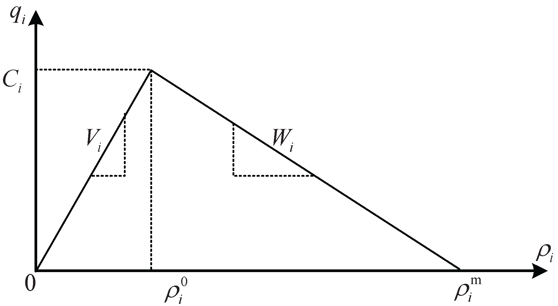
Figure 1. The triangular fundamental diagram.
Information 08 00095 g001
Figure 2. The outer ring of Beijing’s second ring freeway (from Google Maps). The points A and B are marked as the first on-ramp and the first off-ramp, respectively. The segment between A and B is labeled as cell 1 (Note: the Chinese words in this map are just the name of some buildings and will not affect the meaning of this image).
Information 08 00095 g002
Figure 3. Simulated densities. (a) Subsystem 1; (b) Subsystem 2; (c) Subsystem 3; (d) Subsystem 4.
Information 08 00095 g003
Figure 4. Estimated densities. (a) Subsystem 1; (b) Subsystem 2; (c) Subsystem 3; (d) Subsystem 4.
Information 08 00095 g004aInformation 08 00095 g004b
Figure 5. Experimental results. (a) Cell 6; (b) Cell 41; (c) Cell 70; (d) Cell 88.
Information 08 00095 g005
Table 1. Road segment fundamental parameters.
CellVWC ρ 0 ρ m
2, 963186230105535
116618650595580
256018598095585
36, 4061176200102550
576319613599568
5961176158103505
7366186250105560
99, 10065206000102550
Others75196500115582
Table 2. Mean value of mean square error (MSE) for each subsystem.
Subsystem1234
MSE0.12950.13260.13320.1293