Article

Automated Prostate Gland Segmentation Based on an Unsupervised Fuzzy C-Means Clustering Technique Using Multispectral T1w and T2w MR Imaging

1
Dipartimento di Informatica, Sistemistica e Comunicazione (DISCo), Università degli Studi di Milano-Bicocca, Viale Sarca 336, Milano 20126, Italy
2
Istituto di Bioimmagini e Fisiologia Molecolare-Consiglio Nazionale delle Ricerche (IBFM-CNR), Contrada Pietrapollastra-Pisciotto, Cefalù (PA) 90015, Italy
3
Azienda Ospedaliera per l’Emergenza Cannizzaro, Via Messina 829, Catania 95126, Italy
4
Dipartimento di Biopatologia e Biotecnologie Mediche (DIBIMED), Università degli Studi di Palermo, Via del Vespro 129, Palermo 90127, Italy
*
Author to whom correspondence should be addressed.
Information 2017, 8(2), 49; https://doi.org/10.3390/info8020049
Submission received: 4 February 2017 / Revised: 3 April 2017 / Accepted: 24 April 2017 / Published: 28 April 2017
(This article belongs to the Special Issue Fuzzy Logic for Image Processing)

Abstract

:
Prostate imaging analysis is difficult in diagnosis, therapy, and staging of prostate cancer. In clinical practice, Magnetic Resonance Imaging (MRI) is increasingly used thanks to its morphologic and functional capabilities. However, manual detection and delineation of prostate gland on multispectral MRI data is currently a time-expensive and operator-dependent procedure. Efficient computer-assisted segmentation approaches are not yet able to address these issues, but rather have the potential to do so. In this paper, a novel automatic prostate MR image segmentation method based on the Fuzzy C-Means (FCM) clustering algorithm, which enables multispectral T1-weighted (T1w) and T2-weighted (T2w) MRI anatomical data processing, is proposed. This approach, using an unsupervised Machine Learning technique, helps to segment the prostate gland effectively. A total of 21 patients with suspicion of prostate cancer were enrolled in this study. Volume-based metrics, spatial overlap-based metrics and spatial distance-based metrics were used to quantitatively evaluate the accuracy of the obtained segmentation results with respect to the gold-standard boundaries delineated manually by an expert radiologist. The proposed multispectral segmentation method was compared with the same processing pipeline applied on either T2w or T1w MR images alone. The multispectral approach considerably outperforms the monoparametric ones, achieving an average Dice Similarity Coefficient 90.77 ± 1.75, with respect to 81.90 ± 6.49 and 82.55 ± 4.93 by processing T2w and T1w imaging alone, respectively. Combining T2w and T1w MR image structural information significantly enhances prostate gland segmentation by exploiting the uniform gray appearance of the prostate on T1w MRI.

1. Introduction

Prostate cancer is the most frequently diagnosed cancer in men aside from skin cancer, and 180,890 new cases of prostate cancer have been expected in the US during 2016 [1,2]. The only well-established risk factors for prostate cancer are increasing age, a family history of the disease, and genetic conditions. Prostate imaging is still a critical and challenging issue in diagnosis, therapy, and staging of prostate cancer (PCa). Using different imaging modalities, such as Transrectal Ultrasound (TRUS), Computed Tomography (CT) or Magnetic Resonance Imaging (MRI), is dependent on the clinical context. Currently, high-resolution multiparametric MRI has been shown to have higher accuracy than TRUS when used to ascertain the presence of prostate cancer [3]. In [4], MRI-guided biopsy showed a high detection rate of clinically significant PCa in patients with persisting cancer suspicion, also after a previous negative systematic TRUS-guided biopsy, which represents the gold-standard for diagnosis of prostate cancer [5]. In addition, MRI scanning before a biopsy can also serve as a triage test in men with raised serum Prostate-Specific Antigen (PSA) levels, in order to select those for biopsy with significant cancer that requires treatment [6]. For instance, PCa treatment by radiotherapy requires an accurate localization of the prostate. In addition, neighboring tissues and organs at risk, i.e., rectum and bladder, must be carefully preserved from radiation, whereas the tumor should receive a prescribed dose [7]. CT has been traditionally used for radiotherapy treatment planning, but MRI is rapidly gaining relevance because of its superior soft tissue contrast, especially in conformal and intensity-modulated radiation therapy [8].
Manual detection and segmentation of both prostate gland and prostate carcinoma on multispectral MRI is a time-consuming task, which has to be performed by experienced radiologists [9]. In fact, in addition to conventional structural T1-weighted (T1w) and T2-weighted (T2w) MRI protocols, complementary and powerful functional information about the tumor can be extracted [10,11,12] from: Dynamic Contrast Enhanced (DCE) [13], Diffusion Weighted Imaging (DWI) [14], and Magnetic Resonance Spectroscopic Imaging (MRSI) [15,16]. A standardized interpretation of multiparametric MRI is very difficult and significant inter-observer variability has been reported in the literature [17]. The increasing number and complexity of multispectral MRI sequences could overwhelm analytic capabilities of radiologists in their decision-making processes. Therefore, automated and computer-aided segmentation methods are needed to ensure result repeatability.
Accurate prostate segmentation on different imaging modalities is a mandatory step in clinical activities. For instance, prostate boundaries are used in several treatments of prostate diseases: radiation therapy, brachytherapy, High Intensity Focused Ultrasound (HIFU) ablation, cryotherapy, and transurethral microwave therapy [10]. Prostate volume, which can be directly calculated from the prostate Region of Interest (ROI) segmentation, aids in diagnosis of benign prostate hyperplasia and prostate bulging. Precise prostate volume estimation is useful for calculating PSA density and for evaluating post-treatment response. However, these tasks require several degrees of manual intervention, and may not always yield accurate estimates [18]. From a computer science perspective, especially in automatic MR image analysis for prostate cancer segmentation and characterization, the computed prostate ROI is very useful for the subsequent more advanced processing steps [12].
Despite the technological developments in MRI scanners and coils, prostate images are prone to artifacts related to magnetic susceptibility. Although the transition from 1.5 Tesla to 3 Tesla magnetic field strength systems theoretically results in a doubled Signal to Noise Ratio (SNR), it also involves different T1 (spin-lattice) and T2 (spin-spin) relaxation times and greater magnetic field inhomogeneity in the organs and tissues of interest [19,20]. On the other hand, 3 Tesla MRI scanners allow using pelvic coils instead of endorectal coils, obtaining good quality images and avoiding invasiveness as well as prostate gland compression and deformation. Thus, challenges for automatic segmentation of the prostate in MR images include the presence of imaging artifacts due to air in the rectum (i.e., susceptibility artifacts) and large intensity inhomogeneities of the magnetic field (i.e., streaking or shadowing artifacts), the large anatomical variability between subjects, the differences in rectum and bladder filling, and the lack of a normalized “Hounsfield unit” for MRI, like in CT scans [7].
In this paper, an automated segmentation method, based on the Fuzzy C-Means (FCM) clustering algorithm [21], for multispectral MRI morphologic data processing is proposed. This approach allows for prostate segmentation and automatic gland volume calculation. The clustering procedure is performed on co-registered T1w and T2w MR image series. This unsupervised Machine Learning technique, by exploiting a flexible fuzzy model to integrate different MRI sequences, is able to achieve accurate and reliable segmentation results. To the best of our knowledge, this is the first work combining T1w and T2w MR image information to enhance prostate gland segmentation, by taking advantage of the uniform gray appearance of the prostate on T1w MRI, as described in [22]. Segmentation tests were performed on an MRI dataset composed of 21 patients with suspicion of PCa, using volume-based, spatial overlap-based and spatial distance-based metrics to evaluate the effectiveness and the clinical feasibility of the proposed approach.
The structure of the manuscript is the following: Section 2 introduces the background about MRI prostate segmentation methods, Section 3 reports the analyzed multispectral MRI anatomical data and describes the proposed prostate gland segmentation method and the used evaluation metrics, Section 4 illustrates the achieved experimental results, Finally, some discussions and conclusions are provided in Section 5 and Section 6, respectively.

2. Background

This Section summarizes the most representative literature works on prostate segmentation in MRI.
Klein et al. [7] presented an automatic method, based on non-rigid registration of a set of pre-labeled atlas images, for delineating the prostate in 3D MR scans. Each atlas image is non-rigidly registered, employing Localized Mutual Information (LMI) as similarity measure [23], with the target patient image. The registration is performed in two steps: (i) coarse alignment of the two images by a rigid registration; and (ii) fine non-rigid registration, using a coordinate transformation that is parameterized by cubic B-splines [24]. The registration stage yields a set of transformations that can be applied to the atlas label images, resulting in a set of deformed label images that must be combined into a single segmentation of the patient image, considering majority voting (VOTE) and “Simultaneous Truth and Performance Level Estimation” (STAPLE) [25]. The method was evaluated on 50 clinical scans (probably T2w images, but the acquisition protocol is not explicitly reported in the paper), which had been manually segmented by three experts. The Dice Similarity Coefficient (DSC), to quantify the overlap between the automatic and manual segmentations, and the shortest Euclidean distance, between the manual and automatic segmentation boundaries, were computed. The differences among the four used fusion methods are small and mostly not statistically significant. For most test images, the accuracy of the automatic segmentation method was, on a large part of the prostate surface, close to the level of inter-observer variability. With the best parameter setting, a median DSC of around 0.85 was achieved. The segmentation quality is especially good at the prostate-rectum interface, whereas most serious errors occurred around the tips of the seminal vesicles and at the anterior side of the prostate.
Vincent et al. in [26] proposed a fully automatic model-based system for segmenting the prostate in MR images. The segmentation method is based on Active Appearance Models (AAMs) [27] built from 50 manually segmented examples provided by the Medical Image Computing and Computer-Assisted Intervention (MICCAI) 2012 Prostate MR Image Segmentation 2012 (PROMISE12) team [28]. High quality correspondences for the model are generated using a variant of the Minimum Description Length approach to Groupwise Image Registration (MDL-GIR) [29], which finds the set of deformations for registering all the images together as efficiently as possible. A multi-start optimization scheme is used to robustly match the model to new images. To test the performance of the algorithm, DSC, mean absolute distance and the 95th-percentile Hausdorff distance (HD) were calculated. The model was evaluated using a Leave-One-Out Cross Validation (LOOCV) on the training data obtaining a good degree of accuracy and successfully segmented all the test data. The system was used also to segment 30 test cases (without reference segmentations), considering the results very similar to the LOOCV experiment by a visual assessment.
In [30], a unified shape-based framework to extract the prostate from MR images was proposed. First, the authors address the registration problem by representing the shapes of a training set as point clouds. In this way, they are able to exploit the more global aspects of registration via a particle filtering based scheme [31]. In addition, once the shapes have been registered, a cost functional is designed to incorporate both the local image statistics and the learned shape prior (used as constrain to perform the segmentation task). Satisfying experimental results were obtained on several challenging clinical datasets, considering DSC and the 95th-percentile HD, also compared to [32], which employs the Chan-Vese Level Set model [33] assuming a bimodal image.
Martin et al. [34] presented the preliminary results of a semi-automatic approach for prostate segmentation of MR images that aims to be integrated into a navigation system for prostate brachytherapy. The method is based on the registration of an anatomical atlas computed from a population of 18 MRI studies along with each input patient image. A hybrid registration framework, which combines an intensity-based registration [35] and a Robust Point-Matching (RPM) algorithm introducing a geometric constraint (i.e., the distance between the two point sets) [36], is used for both atlas building and atlas registration. This approach incorporates statistical shape information to improve and regularize the quality of the resulting segmentations, using Active Shape Models (ASMs) [37]. The method was validated on the same dataset used for atlas construction, using the LOOCV. Better segmentation accuracy, in terms of volume-based and distance-based metrics, was obtained in the apex zone and in the central zone with respect to the base of the prostate. The same authors proposed a fully automatic algorithm for the segmentation of the prostate in 3D MR images [38]. The approach requires the use of a probabilistic anatomical atlas that is built by computing transformation fields (mapping a set of manually segmented images to a common reference), which are then applied to the manually segmented structures of the training set in order to get a probabilistic map on the atlas. The segmentation procedure is composed of two phases: (i) the processed image is registered to the probabilistic atlas and then a probabilistic segmentation (allowing the introduction of a spatial constraint) is performed by aligning the probabilistic map of the atlas against the patient’s anatomy; and (ii) a deformable surface evolves towards the prostate boundaries by merging information coming from the probabilistic segmentation, an image feature model, and a statistical shape model. During the evolution of the surface, the probabilistic segmentation allows for the introduction of a spatial constraint that prevents the deformable surface from leaking in an unlikely configuration. This method was evaluated on 36 MRI exams. The results showed that introducing a spatial constraint increases the segmentation robustness of the deformable model compared to another one that is only driven by an image appearance model.
Toth et al. [18] used a Multifeature Active Shape (MFA) model [39], which extends ASMs by training the multiple features for each voxel using a Gaussian Mixture Model (GMM) based on the log-likelihood maximization scheme, for estimating prostate volume from T2w MRI. Using a set of training images, the MFA learns the most discriminating statistical texture descriptors of the prostate boundary via a forward feature selection algorithm. After the identification of the optimal image features, the MFA is deformed to accurately fit the prostate border. The MFA-based volume estimation scheme was evaluated on a total 45 T2w in vivo MRI studies, corresponding to both 1.5 Tesla and 3.0 Tesla field strengths. A correlation with the ground truth volume estimations showed that the MFA had higher Pearson’s correlation coefficient values with respect to the current clinical volume estimation schemes, such as ellipsoid, Myschetzky, and prolate spheroid methodologies. In [40], the same research team proposed a scheme to automatically initialize an ASM for prostate segmentation on endorectal in vivo multiprotocol MRI, exploiting MRSI data and identifying the MRI spectra that lie within the prostate. In fact, MRSI is able to measure relative metabolic concentrations and the metavoxels near the prostate have distinct spectral signals from metavoxels outside the prostate. A replicated clustering scheme is employed to distinguish prostatic from extra-prostatic MR spectra in the midgland. The detected spatial locations of the prostate are then used to initialize a multifeature ASM, which employs also statistical texture features in addition to intensity information. This scheme was quantitatively compared with another ASM initialization method for TRUS imaging by Cosìo [41], showing superior average segmentation performance on 388 2D MRI sections obtained from 32 3D endorectal in vivo patient studies.
Other segmentation approaches are also able to segment the zonal anatomy of the prostate [22], differentiating the central gland from the peripheral zone [42]. The method in [43] is based on a modified version of the Evidential C-Means (ECM) clustering algorithm [44], introducing spatial neighborhood information. A priori knowledge of the prostate zonal morphology was modeled as a geometric criterion and used as an additional data source to enhance the differentiation of the two zones. Thirty-one clinical MRI series were used to validate the accuracy of the method, taking into account interobserver variability. The mean DSC was 89% for the central gland and 80% for the peripheral zone, calculated against an expert radiologist segmentation.
Litjens et al. [45] proposed a zonal prostate segmentation approach based on Pattern Recognition techniques. First, they use the multi-atlas segmentation approach in [7] for prostate segmentation, by extending it for using multi-parametric data. T2w MR images and the quantitative Apparent Diffusion Coefficient (ADC) maps were registered simultaneously, In Fact, the ADC map contains additional information on the zonal distribution within the prostate in order to differentiate between the central gland and peripheral zone. Then, for the voxel classification, the authors determined a set of features that represent the difference between the two zones, by considering three categories: anatomy (positional), intensity and texture. This voxel classification approach was validated on 48 multiparametric MRI studies with manual segmentations of the whole prostate. DSC and Jaccard index (JI) showed good results in zonal segmentation of the prostate and outperformed the multiparametric multi-atlas based method in [43] in segmenting both central gland and peripheral zone.
A novel effective method, based on the Fuzzy C-Means (FCM) algorithm [21], is presented in this paper. This soft computing approach is more flexible than the traditional hard clustering version [46]. Differently to the state of the art approaches, this unsupervised Machine Learning technique does not require training phases, statistical shape priors or atlas pre-labeling. Therefore, our method could be easily integrated in clinical practice to support radiologists in their daily decision-making tasks.
Another key novelty is the introduction of T1w MRI in the feature vector, composed of the co-registered T1w and T2w MR image series, fed to the proposed processing pipeline. Although T1w MR images were used in [47] for prostate radiotherapy planning, the authors did not combine both multispectral T2w and T1w MR images using a fusion approach. Their study just highlighted that the Clinical Target Volume (CTV) segmentation results on the T1w and T2w acquisition sequences did not differ significantly in terms of manual CTV. Our work aims to show that the early integration of T2w and T1w MR image structural information significantly enhances prostate gland segmentation by exploiting the uniform gray appearance of the prostate on T1w MRI [22].

3. Patients and Methods

Firstly, the characteristics of the analyzed MRI data are reported. Then, the proposed novel automated segmentation approach on multispectral MRI anatomical images is described. Lastly, the used evaluation metrics are reported.
The proposed method was entirely developed using the MatLab® environment (The MathWorks, Natick, MA, USA).

3.1. Patient Dataset Description

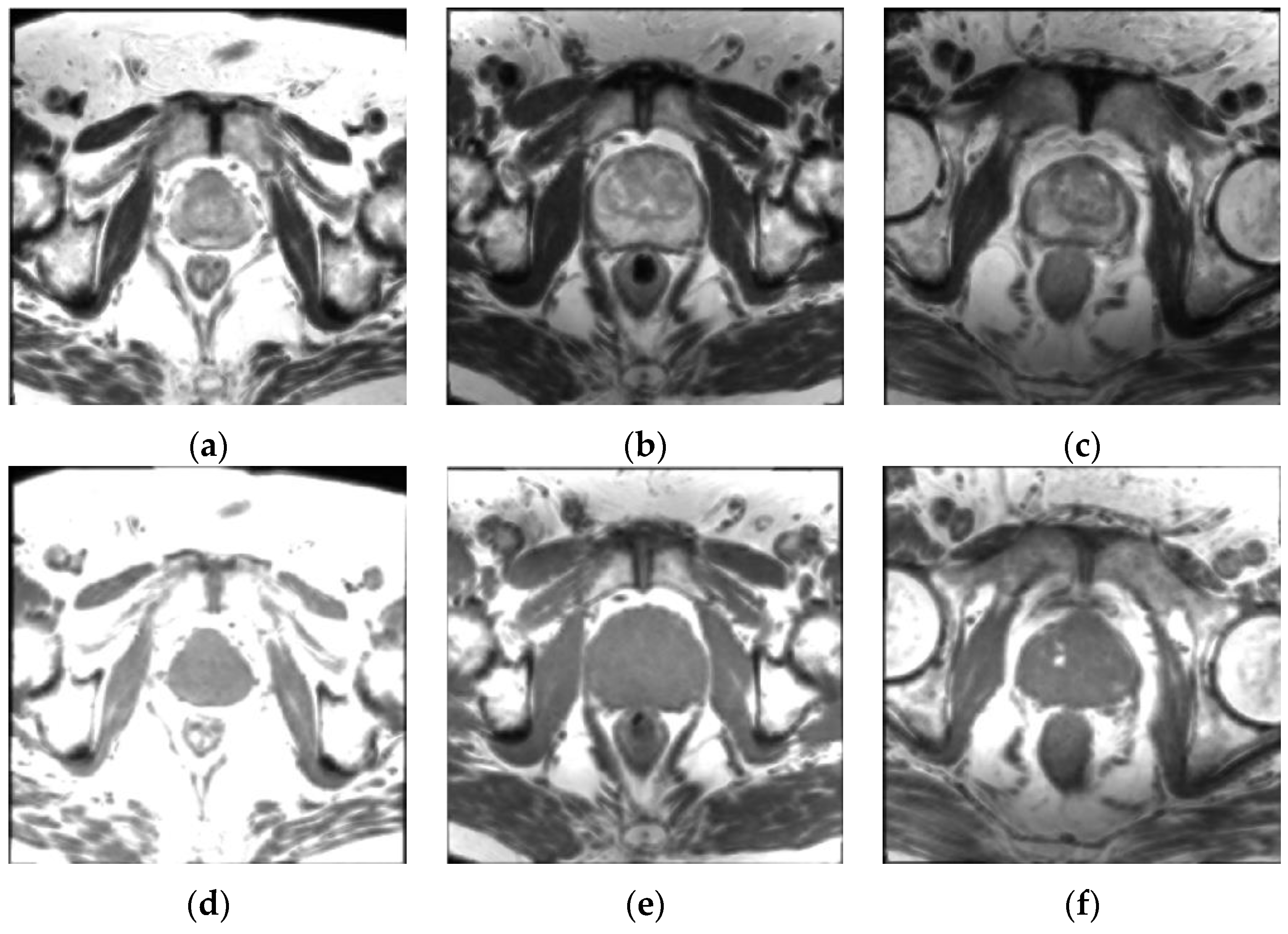
The study was performed on a clinical dataset composed of 21 patients with suspicious PCa. All the analyzed MR images were T1w and T2w Fast Spin Echo (FSE) sequences, acquired with an Achieva 3.0 Tesla MRI Scanner (Philips Medical Systems, Eindhoven, The Netherlands) using a SENSE XL Torso coil (16 elements phased-array pelvic coil), at the Cannizzaro Hospital (Catania, Italy). The total number of the processed 2D MRI slices, in which prostate gland was imaged, was 185. Three pairs of corresponding T1w and T2w MR images are shown in Figure 1.
Imaging data were encoded in the 16 bit (Digital Imaging and COmmunications in Medicine) DICOM format. MRI acquisition parameters are reported in Table 1.
The average age of the examined patients is 65.57 ± 6.42 (53 ÷ 77) years. All the enrolled subjects have clinical suspicion about prostate cancer, due to high PSA levels or digital rectal examination (DRE) for prostate screening. Moreover, the MRI study can be also performed contextually with a previous biopsy, considered as gold-standard, or combined with a further targeted biopsy according to the imaging evidences. In the positive cases, the possible clinical choices are prostatectomy, radiotherapy or chemotherapy.
All the patients signed a written informed consent form.

3.2. The Proposed Method

In this section, an automated segmentation approach of the whole prostate gland from axial MRI slices is presented. The method is based on an unsupervised Machine Learning technique, resulting in an advanced application of the FCM clustering algorithm on multispectral MR anatomical images.
Nowadays, T2w FSE imaging is the standard protocol for depicting the anatomy of the prostate and for identifying prostate cancer considering reduced T2 signal intensity on MRI [48]. These sequences are sensitive to susceptibility artifacts (i.e., local magnetic field inhomogeneities), for instance due to the presence of air in the rectum, which may affect the correct detection of tissue boundaries [7]. On the other hand, because the prostate has uniform intermediate signal intensity at T1w imaging, the zonal anatomy cannot be clearly identified on T1w MRI series [22]. T1w images are used mainly to determine the presence of hemorrhage within the prostate and seminal vesicles and to delineate the gland boundaries [49]. Nevertheless, T1w MRI is not highly sensitive to prostate cancers as well as to inhomogeneous signal in the peripheral zone or adenomatous tissue in the central gland with possible nodules. We exploit this uniform gray appearance, by combining T2w and T1w prostate MRI, to enhance the clustering classification.
Although the prostate gland is represented in the image Field of View (FOV) center, since the organ to be imaged is always positioned approximately near the isocenter of the principal magnetic field to minimize MRI distortions [50], sometimes it may appear shifted from the center or the patient could be not correctly positioned. This fact could affect segmentation accuracy especially in apical and basal prostate MRI slices, when the MR image center is considered for prostate gland segmentation. To address this issue, a rectangular ROI selection tool is dragged around the prostate by the user for more reliable and precise delineation results [51]. Interactive segmentation is becoming more and more popular to alleviate the problems regarding fully automatic segmentation approaches, which are not always able to yield accurate results by adapting to all possible clinical scenarios [52,53]. Thereby, operator-dependency is reduced but, at the same time, the physician is able to monitor and control the segmentation process. Accordingly, computerized medical image analysis has given rise to many promising solutions, but, instead of focusing on fully automatic computerized systems, researchers are aimed to propose computational techniques to aid radiologists in their clinical decision-making tasks [12].
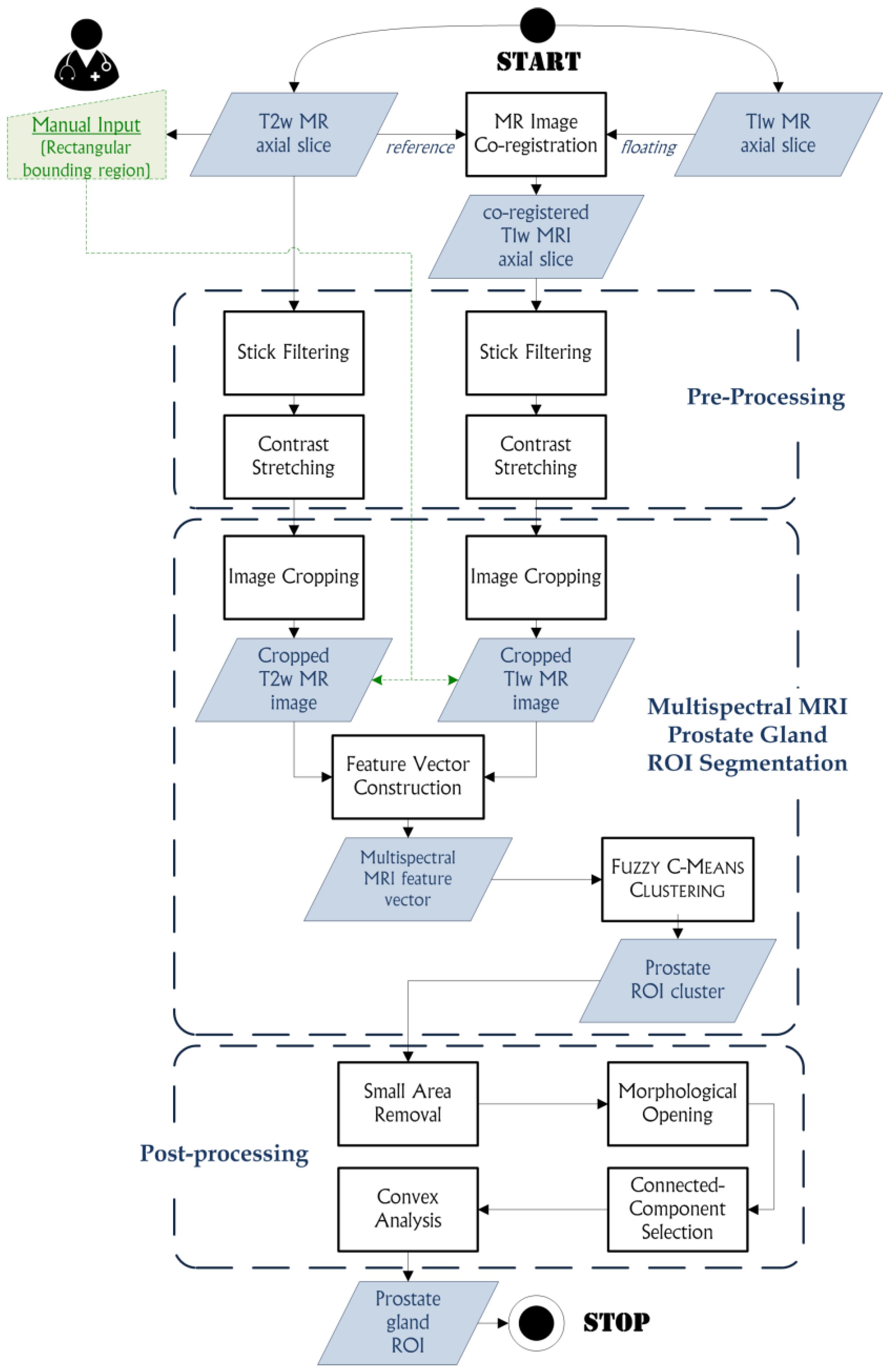
The overall flow diagram of the proposed prostate segmentation method is represented in Figure 2, and a detailed description of each processing phase is provided in the following subsections.

3.2.1. MR Image Co-Registration

Even though T1w and T2w MRI series are included in the same study, they are not acquired contextually because of the different employed extrinsic parameters that determine T1 and T2 relaxation times. Thus, an image co-registration step on multispectral MR images is required. Moreover, T1w and T2w images have different FOVs, in terms of pixel spacing and matrix size (see Table 1 in Section 3.1). However, in our case a 2D image registration method is effective because T1w and T2w MRI sequences are composed of the same number of slices and have the same slice thickness and interslice spacing values.
Image co-registration is accomplished by using an iterative process to align a moving image (T1w) along with a reference image (T2w). In this way, the two images will be represented in the same reference system, so enabling quantitative analysis and processing on fused imaging data. T2w MRI was considered as reference image, to use its own reference system in the following advanced image analysis phases, which are planned in the near future, for differentiating prostate anatomy and for PCa detection and characterization, by processing also functional data (i.e., DCE, DWI, and MRSI).
In intensity-based registration techniques, the accuracy of the registration is evaluated iteratively according to an image similarity metrics. We used Mutual Information (MI) that is an information theoretic measure of the correlation degree between two random variables [54]. High mutual information means a large reduction in the uncertainty (entropy) between the two probability distributions, revealing that the images are likely better aligned [55]. An Evolutionary Strategy (ES), using a one-plus-one optimization configuration, is exploited to find a set of transformations that yields the optimal registration result. In this optimization technique, both the number of parents and the population size (i.e., number of offspring) are set to one [56]. Affine transformations, which combine rigid-body transformations (i.e., translations and rotations) with scaling and shearing, are applied to the moving T1w image to be aligned against the reference T2w image [57].

3.2.2. Pre-Processing

Pre-processing steps are needed for MR image denoising, while preserving relevant feature details such as organ boundaries, and enhance the FCM clustering process. These operations are applied on T2w and the corresponding co-registered T1w input MR series in the same study.
Firstly, stick filtering is applied to efficiently remove the speckle noise that affects MR images [58,59]. The main source of noise in MRI is the thermal noise in the patient [60], influencing both real and imaginary channels with additive white Gaussian noise [61]. The MR image is then reconstructed by computing the inverse discrete Fourier transform of the raw data, resulting in complex white Gaussian noise. The magnitude of the reconstructed MR image is commonly used for visual inspection and for automatic computer analysis [62]. The magnitude of the MRI signal follows a Rician distribution, since it is calculated as the square root of the sum of the squares of two independent Gaussian variables. In low intensity (dark) regions of the magnitude image, the Rician distribution tends to a Rayleigh distribution and in high intensity (bright) regions it tends to a Gaussian distribution [63]. This implies a reduced image contrast, since noise increases the mean value of pixel intensities in dark image regions [62]. By considering a local neighborhood around each pixel, the intensity value of the current pixel is replaced by the maximum of all the stick projections, which are calculated by the convolution of the input image with a long narrow average filter at various orientations [58,59]. Using a stick filter with odd length L and thickness T < L , the square L × L neighborhood can be decomposed into 2 L 2 possible stick projections. Thereby, smoothing is performed on homogeneous regions, while preserving resolvable features and enhancing weak edges and linear structures, without producing too many false edges [64]. Stick filtering parameters are a good balance: the sticks have to be short enough that they can approximate the edges in images, but long enough that the speckle along the sticks is uncorrelated. Therefore, the projections along the sticks can smooth out speckle but not damage real edges in the image. Experimentally, considering the obtained filtering results to be the most suitable input for the Fuzzy C-Means clustering algorithm and enhance the achieved classification, the selected stick filter parameters are: stick length L = 5 pixels; stick thickness T = 1 pixel. All types of low-pass filtering reduce image noise, by removing high-frequency components of the MR signal. This could cause difficulties in tumor detection. Even though this smoothing operation could cause difficulties in cancer detection, our method is tailored for prostate gland segmentation alone and other pre-processing strategies could be employed for a better prostate cancer delineation.
Afterwards, a contrast stretching operation is applied by means of a linear intensity transformation that converts the input intensities into the full dynamic range, in order to improve the subsequent segmentation process. The range of intensity values of the selected part is expanded to enhance the prostate ROI extraction. Thereby, a contrast stretching operation is applied through the global intensity transformation in Equation (1).
s = T ( r ) : = { 0 if r < r min r r min r max r min if r min r r max 1 if r > r max ,
where r is the initial pixel value, s is the pixel value after the transformation, and r min and r max are the minimum and the maximum values of the input image, respectively. This linear normalization converts input intensity r values into the output values s [ 0 , 1 ] . This operation implies an expansion of the values between r min and r max , improving detail discrimination. Since the actual minimum and the maximum intensity values of the MR input were considered as r min and r max , respectively, no regions can have intensity outside of the cut-off values. Thus, no image content or details (e.g., tumors or nodules) could be missed during the following detection phases.
The application of the pre-processing steps is shown in Figure 3. The image noise is visibly suppressed in order to have a more suitable input for the subsequent clustering process, thus extracting the prostate ROI more easily.
To quantitatively justify the selected smoothing operation, we calculated the SNR values on the prostate gland ROI segmentation results for the entire MRI dataset. Since we masked the different MR images with the corresponding prostate gland ROIs, forcing the background to uniform black, the SNR was computed, in compliance with routine MRI quality assurance testing [65], as: S N R = μ R O I / σ R O I , where μ R O I and σ R O I are the average value and the standard deviation of the signal inside the ROI, respectively. After the MR image co-registration step, we evaluated and compared SNR by multiplying pixel-by-pixel each ROI binary mask with the corresponding:
  • original T1w and T2w MR images;
  • T1w and T2w MR images pre-processed with stick filtering (length L = 5 , thickness T = 1 );
  • T1w and T2w MR images filtered with 3 × 3 and 5 × 5 Gaussian kernels;
  • T1w and T2w MR images filtered with 3 × 3 and 5 × 5 average kernels.
For a fair comparison, in all cases, we normalized pixel intensities in [ 0 , 1 ] using a linear stretching transformation, also to be consistent with the proposed pipeline. SNR values achieved on the T2w as well as on the co-registered T1w images are reported in Table 2. As it can be seen, the images pre-processed with stick filtering achieved the highest SNR in both T1w and T2w MRI series.
These pre-processing steps are designed ad hoc to improve the detection of the whole prostate gland. In fact, the main objective of the proposed approach is to accurately delineate the whole prostate and no processing steps for tumor detection are presented. The proposed method yields a prostate gland ROI binary mask, which could be directly employed in a subsequent masking step for a prostate cancer detection methodology by analyzing the corresponding original MR images (also using other pre-processing operations) represented in the same reference system.

3.2.3. Multispectral MRI Prostate Gland ROI Segmentation Based on the FCM Algorithm

Machine Learning studies computer algorithms that can learn automatically complex relationships or patterns from empirical data (i.e., features) and are able to make accurate decisions [66]. Nowadays, Machine Learning plays a key role in radiology applications, helping physicians in their own decision-making tasks on medical imaging data and radiology reports [67]. In Pattern Recognition, features are defined as measurable quantities that could be used to classify different regions [68]. The feature vector, which can include more than one feature, is constructed by concatenating corresponding pixels on T2w and T1w MR images, after the image co-registration step, in an early integration scheme.
An input dataset is partitioned into groups (regions), and each of them is identified by a centroid. The resulting clusters are always represented by connected-regions with unbroken edges. The goal of unsupervised clustering methods is to determine an intrinsic partitioning in a set of unlabeled data, which are associated with a feature vector. Distance metrics are used to group data into clusters of similar types and the number of clusters is assumed to be known a priori [10].
The Fuzzy C-Means (FCM) cluster analysis is an unsupervised technique from the field of Machine Learning [21,69]. An input dataset is partitioned into groups (regions), and each of them is identified by a centroid. The resulting clusters are always represented by connected-regions with unbroken edges.
Formally, as introduced by Bezdek et al. [21], the FCM algorithm aims to divide a set X = { x 1 , x 2 , , x N } composed of N objects (statistical samples represented as feature vectors belonging to n-dimensional Euclidean space n ) into C clusters (partitions of the input dataset). In contrast to the K-Means algorithm [70] that yields a “hard” clustering output, where each feature vector is assigned to exactly one group, the FCM algorithm defines a fuzzy partition P using a fuzzy set family P = { Y 1 , Y 2 , , Y C } . This “soft” classification scheme allows each object to belong to multiple clusters with varying degrees of membership [71]. In mathematical terms, the matrix U = [ u i k ] C × N . denotes a fuzzy C-partition of the set X by means of C membership functions u i : X [ 0 , 1 ] , whose values u i k : = u i ( x k ) [ 0 , 1 ] are interpreted as grades of membership of each element x k to the ith fuzzy set (i.e., the cluster Y i ) and have to satisfy the constraints in Equation (2):
{ 0 u i k 1 i = 1 C u i k = 1 ,   k { 1 , , N } 0 < k = 1 N u i k < N ,   i { 1 , , C } .
Briefly, the sets of all hard and fuzzy C-partitions of the input dataset X are defined by Equations (3) and (4), respectively:
M h a r d = { U C × N : u i k { 0 ,   1 } }
M f u z z y = { U C × N : u i k [ 0 ,   1 ] }
where M f u z z y extends and enhances information provided by M h a r d , by implementing a more flexible method. Although hard clustering works well on compact and well-separated groups of data, in many real-world situations clusters overlap and assigning them with gradual memberships using a soft computing approach may be more appropriate [46].
Computationally, the FCM algorithm assigns to the sample x k the membership function values using the relative distance (considering pixel vicinity or intensity value similarity, in digital imaging) of x k from the C prototype points V = { v 1 , v 2 , , v C } , which identify centroids of the C clusters. This clustering algorithm relies on an optimization procedure concerning the following Objective Function (5), which is a generalized least-squared errors functional:
J m ( U , V ; X ) : = i = 1 C k = 1 N ( u i k ) m d i k   ,
where
  • m is the fuzzification constant (weighting exponent: 1 m < ) that controls the fuzziness of the classification process. If m = 1 , the FCM algorithm approximates hard version. In general, the higher the m value the greater will be the fuzziness degree (the most common value is m = 2 ).
  • U is the fuzzy C-partition of the set X ( U M f u z z y ).
  • d i k = x k v i 2 is the squared distance between the elements x k and v i , computed through an induced norm on n (usually the Euclidean 2 norm).
Therefore, the dataset X is partitioned by iteratively searching for the optimal fuzzy partition P , defined as the pair ( U ^ , V ^ ) that locally minimizes the objective function J m . During each iteration t , the centroid values of the prototype set V ^ ( t ) and the elements of the matrix U ^ ( t ) are updated according to (6) and (7), respectively:
v ^ i ( t ) = j = 1 N ( u ^ i j ( t ) ) m x j j = 1 N ( u ^ i j ( t ) ) m
u ^ i k ( t ) = ( j = 1 C ( x k v ^ i ( t ) x k v ^ j ( t ) ) 2 m 1 ) 1 ,   with   m > 1   and   x k v ^ j ( t )   j , k
At every iteration, each object x k is compared with the elements of the centroid vector and is then assigned to the nearest cluster. The process stops when the convergence condition (i.e., the matrix norm distance between U ^ ( t + 1 ) and U ^ ( t ) is less than a fixed threshold ε ) or the maximum number of iterations T max is reached. Considering the previous theoretical description of the FCM clustering technique, the algorithm, employed for prostate gland ROI segmentation on multispectral MRI anatomical data, can be outlined as in Algorithm 1 pseudo-code box. In order to reproduce our FCM implementation, the parameter setting is the following: C = 3 , m = 2 , ε = 10 5 , and T max = 100 .
Algorithm 1. Pseudo-code of the Fuzzy C-Means clustering algorithm used for prostate gland ROI segmentation on multispectral MRI anatomical data.
Input:
Multispectral MRI anatomical data X = { x 1 , x 2 , , x N } , where each feature vector x i = ( I T 2 w ( x , y ) I T 1 w ( x , y ) ) is constructed by concatenating the intensity values I T 2 w ( x , y ) and I T 1 w ( x , y ) corresponding to the same pixel coordinates ( x , y ) on co-registered T2w and T1w cropped MR images, respectively
Output:
Fuzzy partition into C clusters M f u z z y = { U C × N : u i k [ 0 , 1 ] }
Parameters:
C = 3 , m = 2 , ε = 10 5 , T max = 100
1.
/* Initialization using a uniform pseudorandom number generator UNIF ( 0 , 1 ) */
2.
u i j UNIF ( 0 , 1 ) , u i j U ( 0 ) ;
3.
v i , k UNIF ( 0 , 1 ) ,   v i V ( 0 ) , k [ 1 , 2 , , C ] ;
4.
/* Iterate until convergence is not achieved or the maximum number of iteration is reached */
5.
while ( U ^ ( t + 1 ) U ^ ( t ) 2 > ε   or   t T max ) do
6.
for each feature vector x k X
7.
  /* Update the centroids V ^ ( t + 1 ) and the membership matrix U ^ ( t ) according to Eqs. (6) and (7)*/
8.
   V ^ ( t ) V ^ ( t + 1 ) ; U ^ ( t ) U ^ ( t + 1 ) ; t = t + 1 ;
9.
  Assign each feature vector x k to the cluster identified by the nearest value in the centroids V ^ ( t ) ;
10.
end for
11.
end while
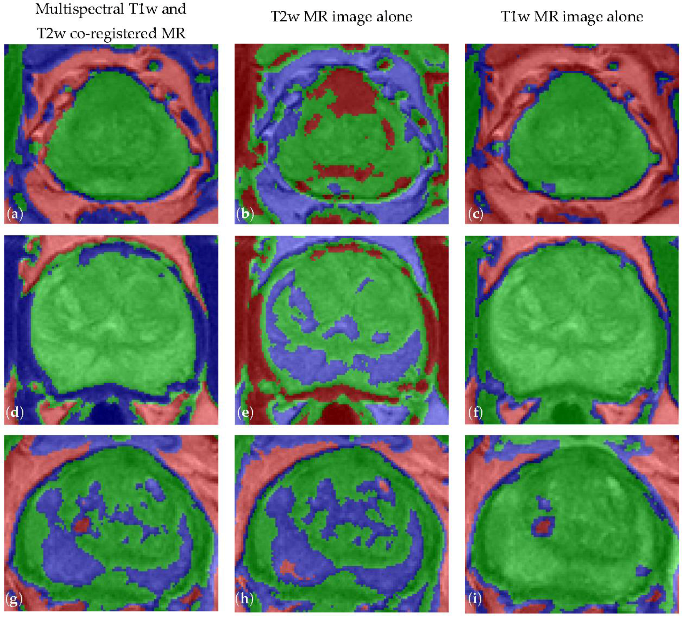
The clustering procedure is performed on the feature vector composed of corresponding T2w and T1w pixel values. The cluster number is always set to C = 3 , by considering both structural and morphologic properties of the processed prostate MR images. In fact, three different classes can essentially be seen by visual inspection according to gray levels. This choice was also justified and endorsed by experimental trials. Figure 4 shows the clustering results achieved by the FCM algorithm with three classes during the prostate gland ROI segmentation stage. It is appreciable how the FCM clustering output on multispectral MRI data considerably enhances the results achieved by processing either T1w or T2w images alone. Especially, the introduction of T1w imaging, in the feature vector construction step, yields a more uniform overall clustering output in the prostate ROI cluster. The resulting feature vector helps decisively to separate the ROI from the other surrounding tissues and organs (i.e., bladder, rectum, seminal vesicles, and levator ani muscle).
As visible in Figure 5b,e,h, FCM clustering on T2w images alone often does not detect the whole prostate gland because of the irregularities due to the prostate zonal anatomy or cancer. However, even though FCM algorithm on T1w images alone obtains more regular clusters, it can also include external regions that can affect the final ROI segmentation results (see Figure 4f,i). Therefore, performing the segmentation on the co-registered T1w and T2w MR image is the best solution for prostate gland segmentation. After the defuzzification step, which consists in assigning the pixels to the cluster with the greatest membership value, the prostate ROI cluster is identified.

3.2.4. Post-Processing

A sequence of morphological operations [72,73] is applied to the obtained ROI cluster to resolve possible ambiguities resulting from the clustering process and to improve the quality of the segmented prostate gland ROI. According to Figure 2, the post-processing steps are the following:
  • A small area removal operation is employed to delete any unwanted connected-components, whose area is less than 500 pixels, which are included into the ROI cluster. These small regions can have similar gray levels to the prostate ROI and were classified into the same cluster by the FCM clustering algorithm. The areas less than 500 pixels certainly do not represent the prostate ROI, since the prostate gland in MRI slices is always characterized by a greater area, regardless of the used acquisition protocol. Thus, these small areas can be removed from the prostate ROI cluster to avoid a wrong connected-component selection in the next processing steps.
  • A morphological opening, using a 5 × 5 pixel square structuring element, is a good compromise between precision in the actual detected contours and capability for unlinking poorly connected regions to the prostate ROI.
  • Connected-component selection, using a flood-fill algorithm [73], determines the connected-component that is the nearest to the cropped image center, since the prostate is always located at the central zone of the cropped image.
  • Convex analysis of the ROI shape since the prostate gland appearance is always convex. A convex hull algorithm [74] is suitable to envelope the segmented ROI into the smallest convex polygon that contains it, so considering possible adjacent regions excluded by the FCM clustering output. Finally, a morphological opening operation with a circular structuring element, is performed for smoothing prostate ROI boundaries. The used circular structuring element with 3 pixel radius allows for smoother and more realistic ROI boundaries without deteriorating significantly the output yielded by the FCM clustering. Accordingly, the value of the radius does not affect the segmentation results and it is not dependent on image resolution.

3.3. Segmentation Evaluation Metrics

In this section, the definitions of the used volume-based, spatial overlap-based and spatial distance-based metrics are reported, according to the formulations presented in [75,76]. These supervised evaluation metrics (i.e., empirical discrepancy methods) are intended to determine the accuracy achieved by a proposed computer-assisted segmentation method against a gold-standard [77]. The reference gold-standard was defined on T2w FSE MRI series (which are generally used in clinical practice, as reported in [48]) by a radiologist highly specialized in urology using the typical manual contouring procedure in clinical practice. In order to obtain more precise and smoother boundaries, a graphics tablet was employed as input pointing device.
Although these boundaries cannot be considered as a perfect “ground truth” because of inter-observer variability [47], prostate gland ROI delineation is less dependent on the operator than prostate cancer detection that requires a more careful diagnosis, involving deeper decision-making processes due to the greater variability of possible pathological scenarios. Thereby, cognitive biases that could affect the diagnostic task are reduced in the case of prostate gland segmentation thanks to the well-known anatomical constraints in the pelvic district. Actually, a gold-standard by a single experienced physician is adequate and generally utilized in literature for assessing quantitatively the accuracy of computer-assisted prostate MRI segmentation approaches.

3.3.1. Volume-Based Metrics

Accurate prostate volume measurement is crucial in diagnostic phases. Therefore, the volume V A computed automatically by the proposed method, should be compared with the actual volume V T , contoured manually by an expert radiologist.
First, to evaluate either overestimation or underestimation of the automated volume measurements with respect to the reference measure, the absolute average volume difference ( A V D ) between the V A and V T values is calculated as:
A V D = abs ( V A V T ) V T .
However, the quantitative measure that best points out the similarity between the volumes V A and V T is the volumetric similarity ( V S ), namely the absolute difference between volumes divided by the volume sum (9):
V S = 1 abs ( | V A | | V T | ) | V A | + | V T | = 1 V D ,
where V D is the volumetric distance and | | indicates the volume cardinality (in terms of the segmented voxels).

3.3.2. Spatial Overlap-Based Metrics

Volume-based metrics do not take into account the intersection between the automatically V A and the manually V T segmented volumes at all. Therefore, overlap-based metrics must be considered.
Spatial overlap-based metrics compare the regions ( R A ) segmented automatically by the method being evaluated against the real measurement (manual segmentation performed by an experienced physician, R T ). According to the confusion matrix, the regions containing “true positives” (TP), “false positives” (FP), “false negatives” (FN), and “true negatives” (TN), are, respectively, represented by Equations (10)–(13):
R T P = R A R T
R F P = R A R T
R F N = R T R A
R T N = I M R I R T R A
The following indices are defined.
  • Dice similarity coefficient ( D S C ) is the most used statistic in validating medical volume segmentations:
    D S C = 2 | R T P | | R A | + | R T | × 100 %
  • Jaccard index ( J I ) is another similarity measure, which is the ratio between the cardinality of the intersection and the cardinality of the union calculated on the two segmentation results:
    J I = | R A R T | | R A R T | × 100 % = D S C 2 D S C
    As can be seen in Equation (15), J I is strongly related to D S C . Moreover D S C is always larger than J I except at extrema { 0 % , 100 % } , where they take equal values.
  • Sensitivity, also called True Positive Ratio ( T P R ), measures the portion of positive (foreground) pixels correctly detected by the proposed segmentation method with respect to the gold-standard segmentation:
    S e n s i t i v i t y = T P R = | R T P | | R T P + R F N | × 100 %
  • Specificity, also called True Negative Ratio ( T N R ), indicates the portion of negative (background) pixels correctly identified by the automatic segmentation against the gold-standard segmentation:
    S p e c i f i c i t y = T N R = | R T N | | R T N + R F P | × 100 %
  • False Positive Ratio ( F P R ) denotes the presence of false positives compared to the reference region:
    F P R = | R F P | | R F P + R T N | × 100 %
  • False Negative Ratio ( F N R ) is analogously defined as:
    F N R = | R F N | | R F N + R T P | × 100 %

3.3.3. Spatial Distance-Based Metrics

Overlap-based metrics are well-suited for measuring the accuracy of a computer-assisted segmentation method compared to the “ground truth” segmentation, but they are also susceptible to differences between the positions of segmented regions and strongly dependent on their own size. Hence, to take into account the spatial position of the voxels, distance-based metrics are highly recommended. In particular, they must be utilized when the boundary delineation is critical, such as in target segmentation for radiation therapy or HIFU ablation.
This leads to the need to quantify the distance between the boundaries computed by the proposed segmentation method and the ones delineated by the expert, which are formally defined by the vertices A = { a i : i = 1 , 2 , , K } and T = { t j : j = 1 , 2 , , N } , respectively. The distance between an element of the contour relative to the automatically calculated ROI and the point set T is defined in (20):
d ( a i , T ) = min j { 1 , , N } a i t j .
Accordingly, several measures can be formulated:
  • Mean absolute distance ( M A D ) quantifies the average error in the segmentation process:
    M A D = 1 K i = 1 K d ( a i , T )
  • Maximum distance ( M a x D ) measures the maximum difference between the two ROI boundaries:
    M a x D = max i { 1 , , K } { d ( a i , T ) }
  • Hausdorff distance ( H D ) is a max-min distance between the point sets A and T defined by:
    H D = max { h ( T , A ) , h ( A , T ) }
    where h ( T , A ) = max t T { min a A { d ( t , a ) } } is called the directed Hausdorff distance and d ( t , a ) = t a 2 = k = 1 n ( t k a k ) 2 is the Euclidean distance ( 2 norm) in n .
The measured distances are expressed in pixels to be independent of the spatial resolution among different prostate MRI datasets (i.e., pixel spacing).

4. Experimental Results

To evaluate the accuracy of the proposed segmentation method, several metrics were calculated by comparing the automatically segmented prostate gland ROIs against the manually contoured ones by an experienced radiologist (considered as our “gold-standard”). Supervised evaluation was used to quantify the goodness of the segmentation outputs [75].
The results achieved by the proposed segmentation approach on multispectral T1w and T2w co-registered MR images were also compared by applying the same processing pipeline on the corresponding monoparametric T2w and T1w MR images alone.
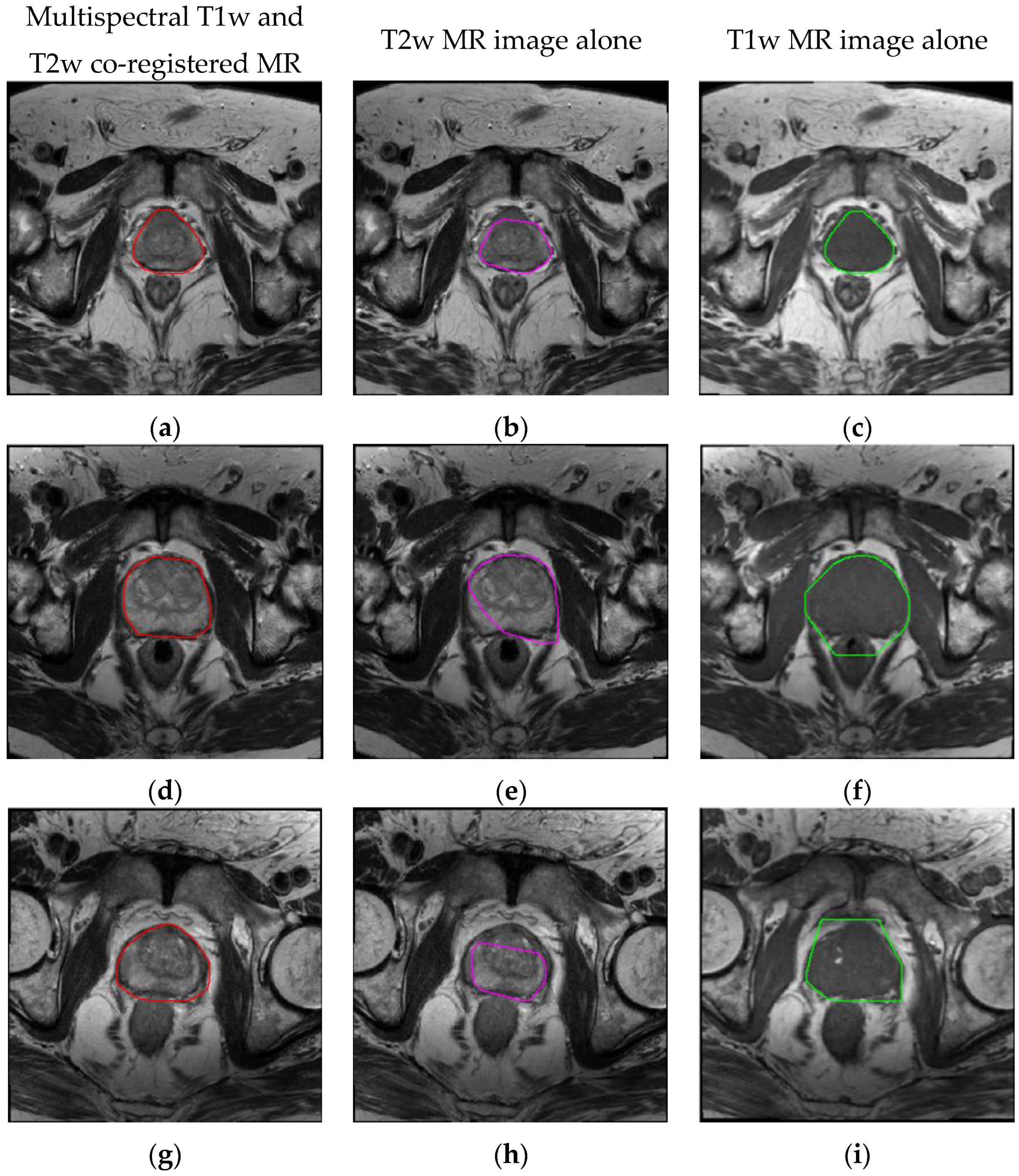
Figure 5 shows three examples of prostate gland ROI obtained by the proposed automated segmentation approach. It is appreciable how correct segmentation results are achieved even with inhomogeneous and noisy input MRI data.
According to Figure 5, it is possible to appreciate the differences by processing multispectral anatomical co-registered images, T2w MR image alone, and T1w image alone. Especially, as shown in Figure 5b,e,h, FCM clustering on T2w images alone often is not able to detect the whole prostate gland because of the irregularities due to the prostate zonal anatomy or cancer. On the other hand, even though FCM clustering on T1w images alone obtains an accurate result in Figure 5c, it can segment also wrong anatomical parts, such as bladder or rectum, because they are imaged with similar gray levels to prostatic gland (Figure 5f,i).
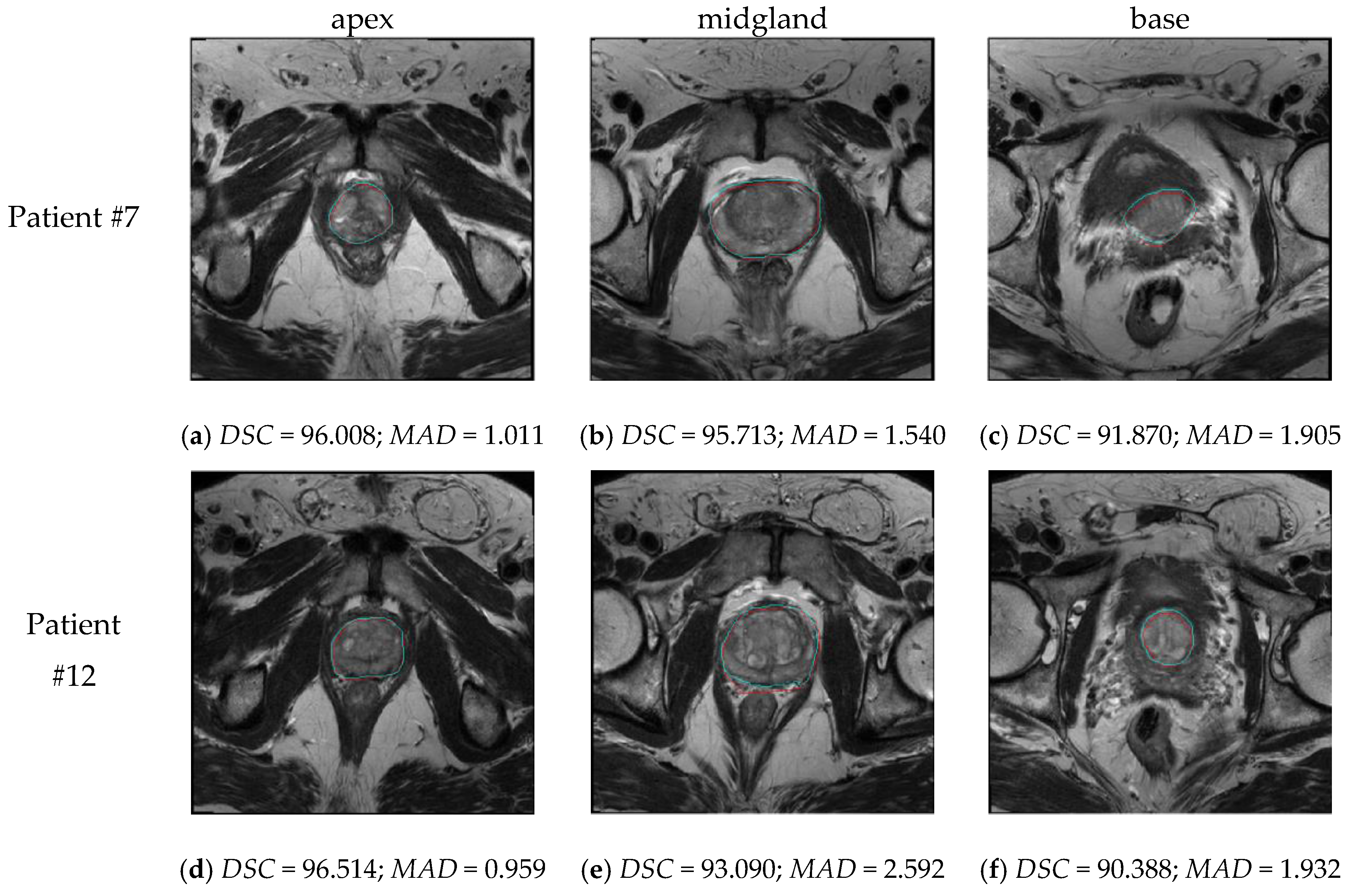
The proposed method is able to correctly segment the midgland and detects reasonably well the apical to the basal prostate regions. An example of the achieved segmentations at the base, center (midgland) and apex of the prostate for the Patients #7 and #12 are shown in Figure 6.
The method is able to separate the prostate gland from seminal vesicles and bladder in basal slices as well as from rectum in central slices.

4.1. Volume Measurements and Volume-Based Metrics Prostate Segmentation Results

Table 3 compares the prostate gland volumes extracted by the proposed automatic method and by the expert physician manually. For each patient, the AVD and VS were calculated. Finally, in the last rows, the average value and the standard deviation for all the examined datasets are reported.
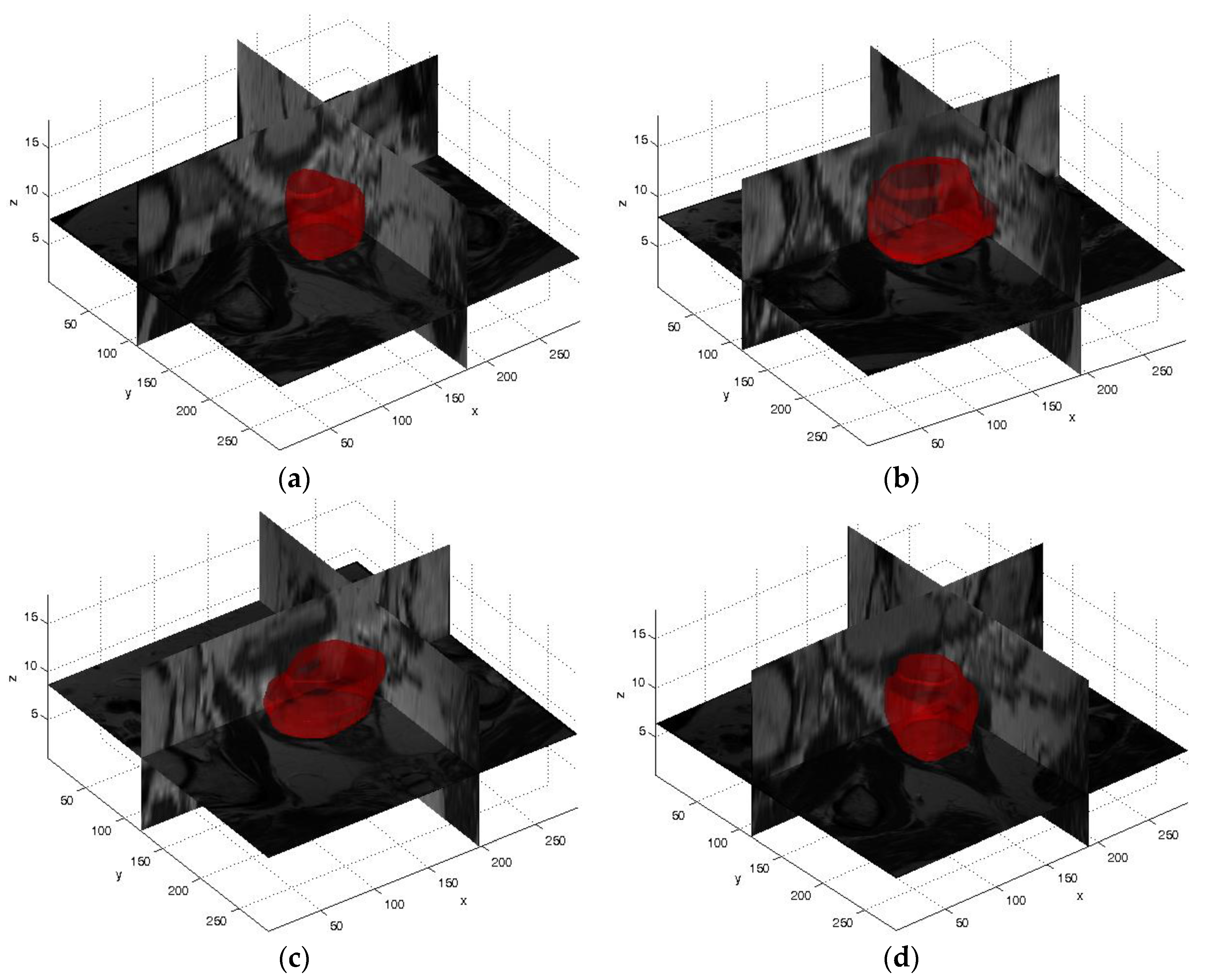
The difference between the automatic and the manual volume measurements is very small, as visible in the AVD values. The high average value and the small standard deviation of the VS metrics corroborate this experimental finding, by proving the reliability of the proposed segmentation approach. For a more complete and intuitive graphical representation, four different instances of volumetric reconstructions of segmented prostate glands are shown in Figure 7. It is worth noting the variety of the prostate gland dimensions and shapes.

4.2. Spatial Overlap-based Metrics Prostate Segmentation Results

Table 4 reports the mean and standard deviation values of the overlap-based metrics obtained in the experimental segmentation tests on 21 MRI series representing prostate gland executing the proposed segmentation method, based on the FCM clustering algorithm, on multispectral MRI anatomical images, T2w images alone, and T1w images alone, respectively.
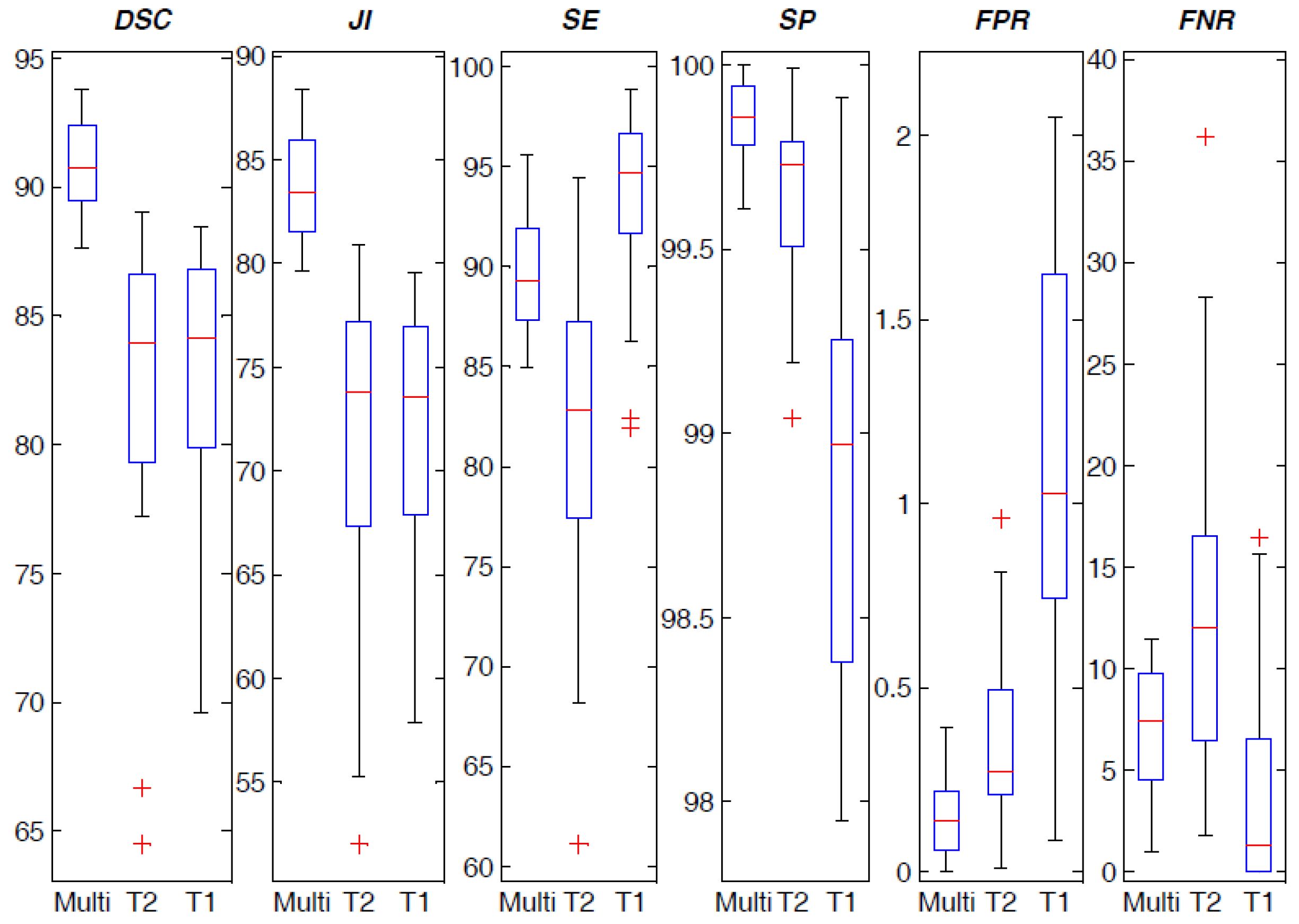
High DSC and JI mean values with very low standard deviation prove the segmentation accuracy and reliability. In addition, Sensitivity and Specificity average values involve the correct detection of the “true” areas and the ability of not detecting “wrong" parts in the segmented prostate gland ROIs, respectively. This is also shown by the obtained FPR and FNR values.
The multispectral approach significantly outperforms the monoparametric ones. The results associated to T1w processing are slightly more sensitive with respect to the proposed multispectral approach, even if they can include also wrong parts as shown by the higher FPR values. However, in all cases, the variance of the results achieved by the monoparametric approaches is higher compared to the proposed multiparametric method. To provide a graphical representation of the statistical distribution of the results, the corresponding boxplots of spatial overlap-based evaluation metrics are also reported in Figure 8.
The short width of the interquartile range (i.e., difference between the third and first quartiles) represented in boxplots implies that the values are considerably concentrated. All index distributions for the multispectral approach do not present outliers, thus demonstrating extremely low statistical dispersion.

4.3. Spatial Distance-Based Metrics Prostate Segmentation Results

Table 5 shows distance-based metrics mean and standard deviation values obtained using the proposed segmentation approach on the dataset composed of 21 patients, by processing multispectral MRI anatomical images, T2w images alone, and T1w images only, respectively. Lower the distance values indicate better segmentation results.
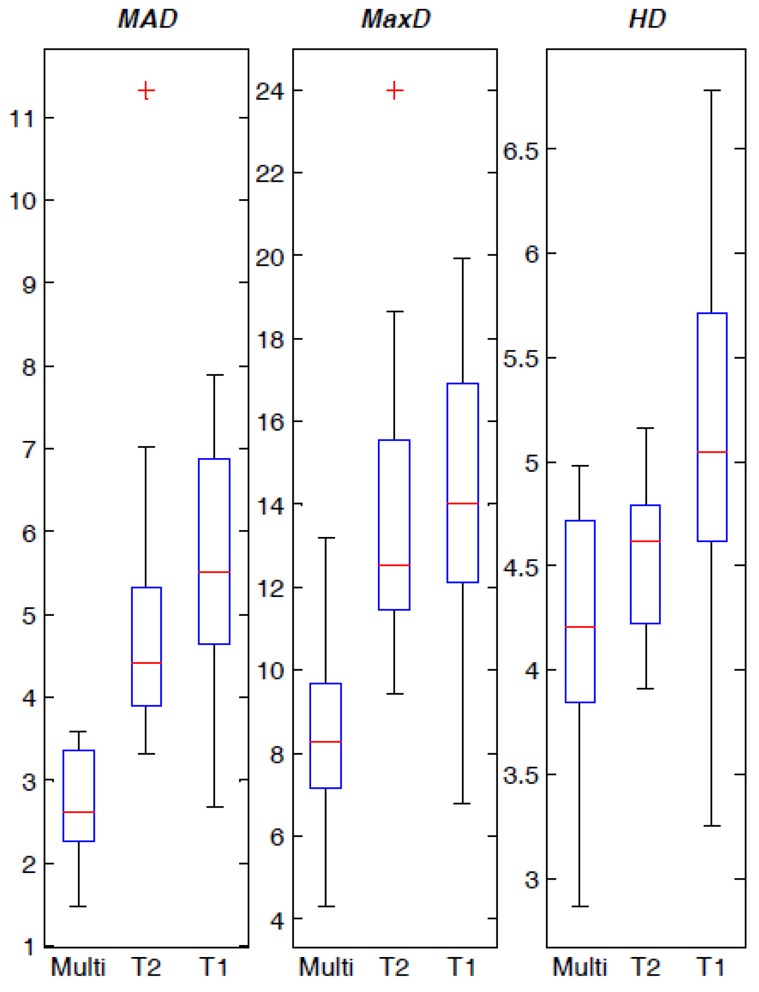
The achieved spatial distance-based indices are consistent with overlap-based metrics. Hence, good performances were obtained also with heterogeneous prostates. As for the spatial overlap-based metrics, also the results obtained on multiparametric MRI anatomical data outperform the monoparametric ones.
Figure 9 depicts the boxplots of the achieved spatial distance-based evaluation metrics.
Observing the boxplots, just a small deviation between the segmentations of the proposed method and those of the experienced radiologist can be denoted. Considering the practical purposes of the proposed prostate gland delineation method for volume calculation in clinical applications, referring to MRI spatial resolution (i.e., isotropic pixel resolution of 0.703 mm in Table 1), the proposed multispectral approach achieved on average 5.965 ± 1.470 mm in the worst case (i.e., MaxD), thus ensuring effective performance. This proves the great accuracy and reliability of the proposed segmentation method in real clinical contexts.

5. Discussion

The proposed approach has proven to give good segmentation results compared to the gold-standard boundaries delineated by an experienced radiologist, as illustrated by the metrics reported in Section 4. Although volume-based metrics do not take into account the intersection, they represent a first and immediate measure of segmentation effectiveness. Just small differences between the automatic and the manual volume measurements were observed, showing the reliability of the proposed segmentation approach for automatic volume calculation in clinical applications. The achieved overlap-based indices, which are characterized by high average values and very low standard deviation, prove the segmentation accuracy, involving the correct detection of the “true” pathological areas as well as the capability of not detecting wrong parts within the segmented prostate. The achieved spatial distance-based metrics agree with the overlap-based ones, corroborating the aforementioned experimental evidences.
The proposed method is based on an unsupervised Machine Learning technique, without requiring any training phase. On the contrary, the other literature works use or combine atlases [7,34,38,45], AAMs [26], or statistical shape priors and ASMs [18,30,34,38,40], which require manual labeling of a significant image sample set performed by expert physicians. In addition, as stated in [38], atlas-based approaches may be affected by serious errors when the processed prostate instances are dissimilar to the atlas, despite the non-rigid registration.
Literature approaches used T2w MR anatomical images, sometimes combined with ADC maps [45] or MRSI data [40]. Our method integrated T1w and T2w MRI anatomical data to enhance clustering segmentation results. To the best of our knowledge, we combined T1w and T2w MR image series for the first time in prostate gland segmentation. As it is stated in [12], the available public prostate MRI datasets for prostate gland segmentation and prostate cancer detection and delineation, such as PROMISE12 [28] and the benchmark proposed in [12], do not provide T1w MR images. Therefore, our method cannot be applied on these public datasets and compared with the prostate MR image segmentation approaches presented at the MICCAI 2012 PROMISE12 challenge, since our aim is to show that concatenating T2w and T1w pixels during the construction of the feature vector in an early integration phase. Although a comparison with state-of-the-art methods could be certainly interesting, it is also unfeasible because atlases should be built and supervised methods with a priori knowledge (such as Active Appearance Models or statistical shape priors) should be trained on our prostate MRI dataset composed of 21 patients. The number of samples is not sufficiently significant to apply suitably supervised Machine Learning techniques or shape-based models without using Leave-One-Out Cross Validation, such as in [26,34].
As shown in Figure 6, our approach is also able to correctly segment apical and basal prostate MRI slices, by differentiating also seminal vesicles (see Figure 6f). The segmentation quality was also good at the prostate-rectum and prostate-bladder interfaces. Whereas a segmentation error of a few millimeters is clinically acceptable at boundaries with muscular tissue, the interfaces with rectum and bladder need to be detected and distinguished very accurately [7]. Moreover, good performances were obtained also with prostate glands imaged as heterogeneous regions (i.e., inhomogeneous signal in the peripheral zone or adenomatous central gland).
The principal experimental finding is that the FCM clustering on multispectral MRI anatomical data considerably enhances the achieved prostate ROI segmentations, by taking advantage of the prostate uniform intermediate signal intensity at T1w imaging [22]. The FCM clustering algorithm on multispectral MR anatomical images allows for more accurate prostate gland ROI segmentation with respect to the clustering results on either T2w or T1w images alone. However, T1w images are often not able to distinguish among different soft tissues. For instance, FCM clustering on T1w images alone is not able to differentiate the prostate-rectum (Figure 5f) or the prostate-muscle (Figure 5i) interfaces. In conclusion, combining and fusing T2w and T1w MRI data, in the feature vector construction step, allow achieving better clustering outputs.
The method was insensitive to variations in patient age, prostate volume and the presence of tumors (i.e., suspicion of cancer in different prostate regions, inhomogeneous signal in the peripheral zone or adenomatous central gland with possible nodules), also considering radiotherapy or chemotherapy treatments, thus increasing its feasibility in clinical practice.

6. Conclusions

In this paper, a novel automated method for prostate segmentation based on the FCM clustering algorithm was proposed. This unsupervised Machine Learning technique was used to effectively support prostate gland delineation, such as in radiation therapy. The developed approach was tested on a dataset composed of 21 patients, considering T2w and T1w MRI series.
Volume-based, spatial overlap-based and distance-based metrics were calculated to evaluate the performance, proving the accuracy of the proposed segmentation approach. The achieved experimental results demonstrated the great robustness of the proposed approach even when MRI series were affected by acquisition noise or artifacts. The good segmentation performance was also confirmed with prostate glands characterized by inhomogeneous signal in the peripheral zone or adenomatous central gland with possible nodules. The developed method could be clinically feasible, by addressing and overcoming typical issues affecting manual segmentation procedures, i.e., time-consuming and operator-dependency.
Future works will be aimed to a more selective segmentation technique, distinguishing between central gland and peripheral gland of the prostate anatomy [22,42]. The advanced segmentation method can be definitely employed in a two-step prostate cancer delineation approach, in order to focus on pathological regions in the central gland and in the peripheral zone.
The overall prostate cancer segmentation method could be integrated into a Computer-Aided Diagnosis (CAD) systems, which include both Computer-Aided Detection (CADe) and Computer-Aided Diagnosis (CADx), enhancing the diagnosis performance of radiologists [12]. In this way, a more accurate PCa staging can be performed, and determining the disease burden might also lead to greater benefit for the patients who underwent treatment [6].

Acknowledgments

This research work was supported by funds from the University of Milano-Bicocca. We would like to thank Lucia Maria Valastro, Maria Gabriella Sabini and Davide D’Urso at Medical Physics Unit of the Cannizzaro Hospital, Catania, Italy, for supplying all the images analyzed in this study.

Author Contributions

Leonardo Rundo and Carmelo Militello conceived the study and wrote the manuscript; Leonardo Rundo, Carmelo Militello and Giorgio Russo analyzed the data; Leonardo Rundo, Carmelo Militello and Salvatore Vitabile designed and performed the experiments; Giorgio Russo and Antonio Garufi provided patient data and validated the achieved experimental results; Salvatore Vitabile, Giancarlo Mauri and Maria Carla Gilardi supervised the design and the development of the proposed study; and all authors read and approved the final manuscript.

Conflicts of Interest

The authors declare no conflict of interest.

References

  1. American Cancer Society, Cancer Facts and Figures 2016. Available online: http://www.cancer.org/acs/groups/content/@research/documents/document/acspc-047079.pdf (accessed on 23 January 2017).
  2. Siegel, R.L.; Miller, K.D.; Jemal, A. Cancer statistics, 2016. CA Cancer J. Clin. 2016, 66, 7–30. [Google Scholar] [CrossRef] [PubMed]
  3. Liu, X.; Langer, D.L.; Haider, M.A.; Yang, Y.; Wernick, M.N.; Yetik, I.S. Prostate cancer segmentation with simultaneous estimation of Markov random field parameters and class. IEEE Trans. Med. Imaging 2009, 28, 906–915. [Google Scholar] [CrossRef] [PubMed]
  4. Roethke, M.; Anastasiadis, A.G.; Lichy, M.; Werner, M.; Wagner, P.; Kruck, S.; Claussen, C.D.; Stenzl, A.; Schlemmer, H.P.; Schilling, D. MRI-guided prostate biopsy detects clinically significant cancer: Analysis of a cohort of 100 patients after previous negative TRUS biopsy. World J. Urol. 2012, 30, 213–218. [Google Scholar] [CrossRef] [PubMed]
  5. Heidenreich, A.; Aus, G.; Bolla, M.; Joniau, S.; Matveev, V.B.; Schmid, H.P.; Zattoni, F. EAU guidelines on prostate cancer. Eur. Urol. 2008, 53, 68–80. [Google Scholar] [CrossRef] [PubMed]
  6. Ahmed, H.U.; Kirkham, A.; Arya, M.; Illing, R.; Freeman, A.; Allen, C.; Emberton, M. Is it time to consider a role for MRI before prostate biopsy? Nat. Rev. Clin. Oncol. 2009, 6, 197–206. [Google Scholar] [CrossRef] [PubMed]
  7. Klein, S.; van der Heide, U.A.; Lips, I.M.; van Vulpen, M.; Staring, M.; Pluim, J.P. Automatic segmentation of the prostate in 3D MR images by atlas matching using localized mutual information. Med. Phys. 2008, 35, 1407–1417. [Google Scholar] [CrossRef] [PubMed]
  8. Villeirs, G.M.; De Meerleer, G.O. Magnetic resonance imaging (MRI) anatomy of the prostate and application of MRI in radiotherapy planning. Eur. J. Radiol. 2007, 63, 361–368. [Google Scholar] [CrossRef] [PubMed]
  9. Hambrock, T.; Vos, P.C.; Hulsbergen-van de Kaa, C.A.; Barentsz, J.O.; Huisman, H.J. Prostate cancer: Computer-aided diagnosis with multiparametric 3-T MR imaging–effect on observer performance. Radiology 2013, 266, 521–530. [Google Scholar] [CrossRef] [PubMed]
  10. Ghose, S.; Oliver, A.; Martí, R.; Lladó, X.; Vilanova, J.C.; Freixenet, J.; Mitra, J.; Sidibé, D.; Meriaudeau, F. A survey of prostate segmentation methodologies in ultrasound, magnetic resonance and computed tomography images. Comput. Meth. Prog. Biomed. 2012, 108, 262–287. [Google Scholar] [CrossRef] [PubMed]
  11. Chilali, O.; Ouzzane, A.; Diaf, M.; Betrouni, N. A survey of prostate modeling for image analysis. Comput. Biol. Med. 2014, 53, 190–202. [Google Scholar] [CrossRef] [PubMed]
  12. Lemaître, G.; Martí, R.; Freixenet, J.; Vilanova, J.C.; Walker, P.M.; Meriaudeau, F. Computer-aided detection and diagnosis for prostate cancer based on mono and multi-parametric MRI: A review. Comput. Biol. Med. 2015, 60, 8–31. [Google Scholar] [CrossRef] [PubMed]
  13. Fabijańska, A. A novel approach for quantification of time-intensity curves in a DCE-MRI image series with an application to prostate cancer. Comput. Biol. Med. 2016, 73, 119–130. [Google Scholar] [CrossRef] [PubMed]
  14. Haider, M.A.; van der Kwast, T.H.; Tanguay, J.; Evans, A.J.; Hashmi, A.T.; Lockwood, G.; Trachtenberg, J. Combined T2-weighted and diffusion-weighted MRI for localization of prostate cancer. AJR Am. J. Roentgenol. 2007, 189, 323–328. [Google Scholar] [CrossRef] [PubMed]
  15. Matulewicz, L.; Jansen, J.F.; Bokacheva, L.; Vargas, H.A.; Akin, O.; Fine, S.W.; Shukla-Dave, A.; Eastham, J.A.; Hricak, H.; Koutcher, J.A.; et al. Anatomic segmentation improves prostate cancer detection with artificial neural networks analysis of 1H magnetic resonance spectroscopic imaging. J. Magn. Reson. Imaging 2014, 40, 1414–1421. [Google Scholar] [CrossRef] [PubMed]
  16. Fütterer, J.J.; Heijmink, S.W.; Scheenen, T.W.; Veltman, J.; Huisman, H.J.; Vos, P.; Hulsbergen-van de Kaa, A.C.; Witjes, J.A.; Krabbe, P.F.M.; Heerschap, A.; et al. Prostate cancer localization with dynamic contrast-enhanced MR imaging and proton MR spectroscopic imaging. Radiology 2006, 241, 449–458. [Google Scholar] [CrossRef] [PubMed]
  17. Rosenkrantz, A.B.; Lim, R.P.; Haghighi, M.; Somberg, M.B.; Babb, J.S.; Taneja, S.S. Comparison of interreader reproducibility of the prostate imaging reporting and data system and Likert scales for evaluation of multiparametric prostate MRI. AJR Am. J. Roentgenol. 2013, 201, W612–W618. [Google Scholar] [CrossRef] [PubMed]
  18. Toth, R.; Bloch, B.N.; Genega, E.M.; Rofsky, N.M.; Lenkinski, R.E.; Rosen, M.A.; Kalyanpur, A.; Pungavkar, S.; Madabhushi, A. Accurate prostate volume estimation using multifeature active shape models on T2-weighted MRI. Acad. Radiol. 2011, 18, 745–754. [Google Scholar] [CrossRef] [PubMed]
  19. Caivano, R.; Cirillo, P.; Balestra, A.; Lotumolo, A.; Fortunato, G.; Macarini, L.; Zandolino, A.; Vita, G.; Cammarota, A. Prostate cancer in magnetic resonance imaging: Diagnostic utilities of spectroscopic sequences. J. Med. Imaging Radiat. Oncol. 2012, 56, 606–616. [Google Scholar] [CrossRef] [PubMed]
  20. Rouvière, O.; Hartman, R.P.; Lyonnet, D. Prostate MR imaging at high-field strength: Evolution or revolution? Eur. Radiol. 2006, 16, 276–284. [Google Scholar] [CrossRef] [PubMed]
  21. Bezdek, J.C.; Ehrlich, R.; Full, W. FCM: The fuzzy c-means clustering algorithm. Comput. Geosci. 1984, 10, 191–203. [Google Scholar] [CrossRef]
  22. Choi, Y.J.; Kim, J.K.; Kim, N.; Kim, K.W.; Choi, E.K.; Cho, K.S. Functional MR imaging of prostate cancer. Radiographics 2007, 27, 63–75. [Google Scholar] [CrossRef] [PubMed]
  23. Studholme, C.; Drapaca, C.; Iordanova, B.; Cardenas, V. Deformation-based mapping of volume change from serial brain MRI in the presence of local tissue contrast change. IEEE Trans. Med. Imaging 2006, 25, 626–639. [Google Scholar] [CrossRef] [PubMed]
  24. Rueckert, D.; Sonoda, L.I.; Hayes, C.; Hill, D.L.; Leach, M.O.; Hawkes, D.J. Nonrigid registration using free-form deformations: Application to breast MR images. IEEE Trans. Med. Imaging 1999, 18, 712–721. [Google Scholar] [CrossRef] [PubMed]
  25. Warfield, S.K.; Zou, K.H.; Wells, W.M. Simultaneous truth and performance level estimation (STAPLE): An algorithm for the validation of image segmentation. IEEE Trans. Med. Imaging 2004, 23, 903–921. [Google Scholar] [CrossRef] [PubMed]
  26. Vincent, G.; Guillard, G.; Bowes, M. Fully automatic segmentation of the prostate using active appearance models. In Proceedings of the 15th International Conference on Medical Image Computing and Computer-Assisted Intervention (MICCAI) Grand Challenge: Prostate MR Image Segmentation 2012, Nice, France, 1–5 October 2012; p. 7. [Google Scholar]
  27. Heimann, T.; Meinzer, H.P. Statistical shape models for 3D medical image segmentation: A review. Med. Image Anal. 2009, 13, 543–563. [Google Scholar] [CrossRef] [PubMed]
  28. Litjens, G.; Toth, R.; van de Ven, W.; Hoeks, C.; Kerkstra, S.; van Ginneken, B.; Vincent, G.; Guillard, G.; Birbeck, N.; Zhang, J.; et al. Evaluation of prostate segmentation algorithms for MRI: The PROMISE12 challenge. Med. Image Anal. 2014, 18, 359–373. [Google Scholar] [CrossRef] [PubMed]
  29. Cootes, T.F.; Twining, C.J.; Petrovic, V.S.; Schestowitz, R.; Taylor, C.J. Groupwise construction of appearance models using piece-wise affine deformations. In Proceedings of the 16th British Machine Vision Conference (BMVC), Oxford, UK, 5–8 September 2005; Clocksin, W.F., Fitzgibbon, A.W., Torr, P.H.S., Eds.; Volume 2, pp. 879–888. [Google Scholar]
  30. Gao, Y.; Sandhu, R.; Fichtinger, G.; Tannenbaum, A.R. A coupled global registration and segmentation framework with application to magnetic resonance prostate imagery. IEEE Trans. Med. Imaging 2010, 29, 1781–1794. [Google Scholar] [CrossRef] [PubMed]
  31. Sandhu, R.; Dambreville, S.; Tannenbaum, A. Particle filtering for registration of 2D and 3D point sets with stochastic dynamics. In Proceedings of the IEEE Conference on Computer Vision and Pattern Recognition (CVPR 2008), Anchorage, AK, USA, 23–28 June 2008; pp. 1–8. [Google Scholar]
  32. Tsai, A.; Yezzi, A.; Wells, W.; Tempany, C.; Tucker, D.; Fan, A.; Grimson, W.E.; Willsky, A. A shape-based approach to the segmentation of medical imagery using level sets. IEEE Trans. Med. Imaging 2003, 22, 137–154. [Google Scholar] [CrossRef] [PubMed]
  33. Chan, T.F.; Vese, L.A. Active contours without edges. IEEE Trans. Med. Imaging 2001, 10, 266–277. [Google Scholar] [CrossRef] [PubMed]
  34. Martin, S.; Daanen, V.; Troccaz, J. Atlas-based prostate segmentation using an hybrid registration. Int. J. Comput. Assist. Radiol. Surg. 2008, 3, 485–492. [Google Scholar] [CrossRef]
  35. Hellier, P.; Barillot, C. Coupling dense and landmark-based approaches for nonrigid registration. IEEE Trans. Med. Imaging 2003, 22, 217–227. [Google Scholar] [CrossRef] [PubMed]
  36. Rangarajan, A.; Chui, H.; Bookstein, F.L. The softassign procrustes matching algorithm. In Information Processing in Medical Imaging, Proceedings of the 15th International Conference, IPMI'97, Poultney, VT, USA, 9–13 June 1997; Lecture Notes in Computer Science; Springer: Berlin/Heidelberg, Germany, 1997; Volume 1230, pp. 29–42. [Google Scholar]
  37. Cootes, T.F.; Hill, A.; Taylor, C.J.; Haslam, J. Use of active shape models for locating structures in medical images. Image Vis. Comput. 1994, 12, 355–365. [Google Scholar] [CrossRef]
  38. Martin, S.; Troccaz, J.; Daanen, V. Automated segmentation of the prostate in 3D MR images using a probabilistic atlas and a spatially constrained deformable model. Med. Phys. 2010, 37, 1579–1590. [Google Scholar] [CrossRef] [PubMed]
  39. Cootes, T.F.; Taylor, C.J.; Cooper, D.H.; Graham, J. Active shape models-their training and application. Comput. Vis. Image Underst. 1995, 61, 38–59. [Google Scholar] [CrossRef]
  40. Toth, R.; Tiwari, P.; Rosen, M.; Reed, G.; Kurhanewicz, J.; Kalyanpur, A.; Pungavkar, S.; Madabhushi, A. A magnetic resonance spectroscopy driven initialization scheme for active shape model based prostate segmentation. Med. Image Anal. 2011, 15, 214–225. [Google Scholar] [CrossRef] [PubMed]
  41. Cosío, F.A. Automatic initialization of an active shape model of the prostate. Med. Image Anal. 2008, 12, 469–483. [Google Scholar] [CrossRef] [PubMed]
  42. Hricak, H.; Dooms, G.C.; McNeal, J.E.; Mark, A.S.; Marotti, M.; Avallone, A.; Pelzer, M.; Proctor, E.C.; Tanagho, E.A. MR imaging of the prostate gland: Normal anatomy. AJR Am. J. Roentgenol. 1987, 148, 51–58. [Google Scholar] [CrossRef] [PubMed]
  43. Makni, N.; Iancu, A.; Colot, O.; Puech, P.; Mordon, S.; Betrouni, N. Zonal segmentation of prostate using multispectral magnetic resonance images. Med. Phys. 2011, 38, 6093–6105. [Google Scholar] [CrossRef] [PubMed]
  44. Masson, M.H.; Denœux, T. ECM: An evidential version of the fuzzy c-means algorithm. Pattern Recognit. 2008, 41, 1384–1397. [Google Scholar] [CrossRef]
  45. Litjens, G.; Debats, O.; van de Ven, W.; Karssemeijer, N.; Huisman, H. A pattern recognition approach to zonal segmentation of the prostate on MRI. In Medical Image Computing and Computer-Assisted Intervention—MICCAI 2012, Proceedings of the 15th International Conference on Medical Image Computing and Computer Assisted Intervention, Nice, France, 1–5 October 2012; Springer: Berlin/Heidelberg, Germany, 2012; pp. 413–420. [Google Scholar]
  46. Huang, H.C.; Chuang, Y.Y.; Chen, C.S. Multiple Kernel Fuzzy Clustering. IEEE Trans. Fuzzy Syst. 2012, 20, 120–134. [Google Scholar] [CrossRef]
  47. Pasquier, D.; Lacornerie, T.; Vermandel, M.; Rousseau, J.; Lartigau, E.; Betrouni, N. Automatic segmentation of pelvic structures from magnetic resonance images for prostate cancer radiotherapy. Int. J. Radiat. Oncol. Biol. Phys. 2007, 68, 592–600. [Google Scholar] [CrossRef] [PubMed]
  48. Kurhanewicz, J.; Vigneron, D.; Carroll, P.; Coakley, F. Multiparametric magnetic resonance imaging in prostate cancer: Present and future. Curr. Opin. Urol. 2008, 18, 71–77. [Google Scholar] [CrossRef] [PubMed]
  49. Barentsz, J.O.; Weinreb, J.C.; Verma, S.; Thoeny, H.C.; Tempany, C.M.; Shtern, F.; Padhani, A.R.; Margolis, D.; Macura, K.J.; Haider, M.A.; et al. Synopsis of the PI-RADS v2 guidelines for multiparametric prostate magnetic resonance imaging and recommendations for use. Eur. Urol. 2016, 69, 41–49. [Google Scholar] [CrossRef] [PubMed]
  50. Lagendijk, J.J.W.; Raaymakers, B.W.; Van den Berg, C.A.T.; Moerland, M.A.; Philippens, M.E.; van Vulpen, M. MR guidance in radiotherapy. Phys. Med. Biol. 2014, 59, R349–R369. [Google Scholar] [CrossRef] [PubMed]
  51. Chen, C.; Abdelnour-Nocera, J.; Wells, S.; Pan, N. Usability practice in medical imaging application development. In HCI and Usability for e-Inclusion; Lecture Notes in Computer Science; Springer: Berlin/Heidelberg, Germany, 2009; Volume 5889, pp. 405–415. [Google Scholar]
  52. Boykov, Y.Y.; Jolly, M.P. Interactive graph cuts for optimal boundary & region segmentation of objects in N-D images. In Proceedings of the Eighth IEEE International Conference on Computer Vision (ICCV), Vancouver, BC, Canada, 7–14 July 2001; Volume 1, pp. 105–112. [Google Scholar]
  53. Boykov, Y.Y.; Jolly, M.P. Interactive organ segmentation using graph cuts. In Medical Image Computing and Computer-Assisted Intervention—MICCAI 2000, Proceedings of the Third International Conference on Medical Image Computing and Computer Assisted Intervention, Pittsburgh, PA, USA, 11–14 October 2000; Lecture Notes in Computer Science; Springer: Berlin/Heidelberg, Germany, 2000; Volume 1935, pp. 276–286. [Google Scholar]
  54. Pluim, J.P.W.; Maintz, J.B.A.; Viergever, M.A. Mutual-information-based registration of medical images: A survey. IEEE Trans. Med. Imaging 2003, 22, 986–1004. [Google Scholar] [CrossRef] [PubMed]
  55. Mattes, D.; Haynor, D.R.; Vesselle, H.; Lewellen, T.; Eubank, W. Non-rigid multimodality image registration. In Medical Imaging 2001: Image Processing, Proceedings of the SPIE 4322, San Diego, CA, USA, 17 February 2001; SPIE: Bellingham, WA, USA, 2001; pp. 1609–1620. [Google Scholar]
  56. Styner, M.; Brechbuhler, C.; Szckely, G.; Gerig, G. Parametric estimate of intensity inhomogeneities applied to MRI. IEEE Trans. Med. Imaging 2000, 19, 153–165. [Google Scholar] [CrossRef] [PubMed]
  57. Rundo, L.; Tangherloni, A.; Militello, C.; Gilardi, M.C.; Mauri, G. Multimodal medical image registration using particle swarm optimization: A review. In Proceedings of the 2016 IEEE Symposium Series on Computational Intelligence (IEEE SSCI 2016)—Swarm Intelligence Symposium (SIS), Athens, Greece, 6–9 December 2016; pp. 1–8. [Google Scholar]
  58. Czerwinski, R.N.; Jones, D.L.; O’Brien, W.D. Line and boundary detection in speckle images. IEEE Trans. Image Process. 1998, 7, 1700–1714. [Google Scholar] [CrossRef] [PubMed]
  59. Czerwinski, R.N.; Jones, D.L.; O’Brien, W.D. Detection of lines and boundaries in speckle images-application to medical ultrasound. IEEE Trans. Med. Imaging 1999, 18, 126–136. [Google Scholar] [CrossRef] [PubMed]
  60. Edelstein, W.A.; Glover, G.H.; Hardy, C.J.; Redington, R.W. The intrinsic signal-to-noise ratio in NMR imaging. Magn. Reson. Med. 1986, 3, 604–618. [Google Scholar] [CrossRef] [PubMed]
  61. Macovski, A. Noise in MRI. Magn. Reson. Med. 1996, 36, 494–497. [Google Scholar] [CrossRef] [PubMed]
  62. Pizurica, A.; Wink, A.M.; Vansteenkiste, E.; Philips, W.; Roerdink, B.J. A review of wavelet denoising in MRI and ultrasound brain imaging. Curr. Med. Imaging Rev. 2006, 2, 247–260. [Google Scholar] [CrossRef]
  63. Papoulis, A.; Pillai, S.U. Probability, Random Variables and Stochastic Processes, 4th ed.; McGraw-Hill: New York, NY, USA, 2001. [Google Scholar]
  64. Xiao, C.Y.; Zhang, S.; Cheng, S.; Chen, Y.Z. A novel method for speckle reduction and edge enhancement in ultrasonic images. In Electronic Imaging and Multimedia Technology IV, Proceedings of the SPIE 5637, Beijing, China, 8 November 2004; SPIE: Bellingham, WA, USA, 2005. [Google Scholar]
  65. Firbank, M.J.; Coulthard, A.; Harrison, R.M.; Williams, E.D. A comparison of two methods for measuring the signal to noise ratio on MR images. Phys. Med. Biol. 1999, 44. [Google Scholar] [CrossRef]
  66. Bishop, C.M. Pattern Recognition and Machine Learning (Information Science and Statistics), 1st ed.; Springer: Secaucus, NJ, USA, 2006. [Google Scholar]
  67. Wang, S.; Summers, R.M. Machine learning and radiology. Med. Image Anal. 2012, 16, 933–951. [Google Scholar] [CrossRef] [PubMed]
  68. Lu, J.; Xue, S.; Zhang, X.; Han, Y. A neural network-based interval pattern matcher. Information 2015, 6, 388–398. [Google Scholar] [CrossRef]
  69. Militello, C.; Vitabile, S.; Rundo, L.; Russo, G.; Midiri, M.; Gilardi, M.C. A fully automatic 2d segmentation method for uterine fibroid in MRgFUS treatment evaluation. Comput. Biol. Med. 2015, 62, 277–292. [Google Scholar] [CrossRef] [PubMed]
  70. Kanungo, T.; Mount, D.M.; Netanyahu, N.S.; Piatko, C.D.; Silverman, R.; Wu, A.Y. An efficient k-means clustering algorithm: Analysis and implementation. IEEE Trans. Pattern Anal. Mach. Intell. 2002, 24, 881–892. [Google Scholar] [CrossRef]
  71. Zhang, D.Q.; Chen, S.C. A novel kernelized fuzzy c-means algorithm with application in medical image segmentation. Artif. Intell. Med. 2004, 32, 37–50. [Google Scholar] [CrossRef] [PubMed]
  72. Soille, P. Morphological Image Analysis: Principles and Applications, 2nd ed.; Springer: Secaucus, NJ, USA, 2003. [Google Scholar]
  73. Breen, E.J.; Jones, R.; Talbot, H. Mathematical morphology: A useful set of tools for image analysis. Stat. Comput. 2000, 10, 105–120. [Google Scholar] [CrossRef]
  74. Zimmer, Y.; Tepper, R.; Akselrod, S. An improved method to compute the convex hull of a shape in a binary image. Pattern Recognit. 1997, 30, 397–402. [Google Scholar] [CrossRef]
  75. Taha, A.A.; Hanbury, A. Metrics for evaluating 3D medical image segmentation: Analysis, selection, and tool. BMC Med. Imaging 2015, 15, 1–28. [Google Scholar] [CrossRef] [PubMed]
  76. Fenster, A.; Chiu, B. Evaluation of segmentation algorithms for medical imaging. In Proceedings of the 27th Annual International Conference of the Engineering in Medicine and Biology Society, Shanghai, China, 1–4 September 2005; pp. 7186–7189. [Google Scholar]
  77. Zhang, Y.J. A review of recent evaluation methods for image segmentation. In Proceedings of the Sixth IEEE International Symposium on Signal Processing and Its Applications (ISSPA), Kuala Lumpur, Malaysia, 13–16 August 2001; Volume 1, pp. 148–151. [Google Scholar]
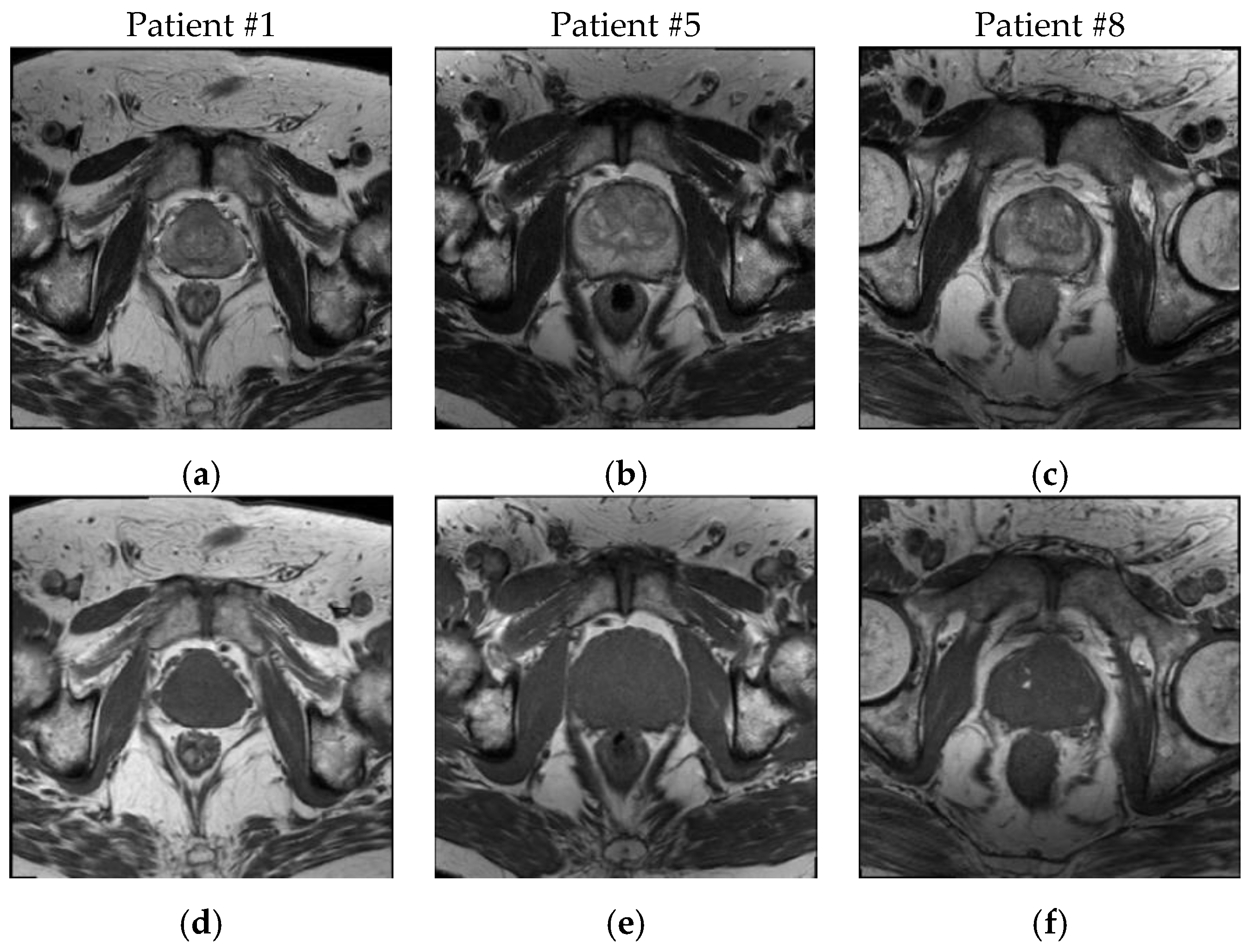
Figure 1. Three instances of input MRI axial slice pairs for the Patients #1, #5 and #8: (ac) T2w MR images; and (df) corresponding T1w MR images.
Information 08 00049 g001
Figure 2. Flow diagram of the proposed prostate gland segmentation method. The pipeline can be subdivided in three main stages: (i) pre-processing, required to remove speckle noise and enhance the FCM clustering process; (ii) FCM clustering on multispectral MR images, to extract the prostate gland ROI; and (iii) post-processing, well-suited to refine the obtained segmentation results.
Information 08 00049 g002
Figure 3. Pre-Processing phase: (ac) T2w images; and (df) corresponding T1w images after pre-processing steps, consisting in stick filtering and linear contrast stretching, on the images in Figure 1.
Information 08 00049 g003
Figure 4. Results of the FCM clustering algorithm with C = 3 for prostate gland ROI segmentation on the input images in Figure 1, by processing different feature vectors: (a,d,g) results on the multispectral T1w and T2w co-registered MR images; (b,e,h) results on T2w MR image alone; and (c,f,i) results on T1w MR image alone. It is possible to appreciate the multispectral MRI contribution with respect to the single series clustering outputs. In all cases, the prostate gland ROI cluster is represented by the green regions. The clusters are superimposed on the original T2w MR image using a transparence with Alpha Blending ( α = 0.40 ).
Information 08 00049 g004
Figure 5. Prostate gland ROI segmentation instances on the axial MRI slices shown in Figure 1 by processing different input MRI data (i.e., feature vectors) of three different patients (one per row): (a,d,g), results obtained on multispectral T1w and T2w co-registered MR image (red contour superimposed on T2w image); (b,e,h), results obtained on T2w MR image alone (magenta contour superimposed on T2w image); and (c,f,i), results obtained on T1w MR image alone (green contour superimposed on T1w image).
Information 08 00049 g005
Figure 6. Examples of segmentation results (red and cyan contours representing the proposed and the manual delineations, respectively, are superimposed on T2w axial prostate MR images) obtained on: apical (a,d); central (b,e); and basal (c,f) slices concerning Patients #7 and #12, respectively. At the bottom of each sub-figure, the values for Dice similarity coefficient (DSC) and mean average distance (MAD) are reported.
Information 08 00049 g006
Figure 7. Tridimensional reconstruction of the segmented prostate gland ROI on the 3D orthogonal tri-planar view for Patients: (a) #1; (b) #5; (c) #7; and (d) #12. Transparent surfaces of the prostate gland are rendered with Alpha Blending ( α = 0.40 ).
Information 08 00049 g007
Figure 8. Boxplots of the spatial overlap-based metrics values achieved by the proposed prostate gland ROI segmentation approach based on the FCM algorithm. From left to right: Dice similarity coefficient (DSC), Jaccard index (JI), Sensitivity (SE), Specificity (SP), False Positive Ratio (FPR), and False Negative Ratio (FNR). The lower and the upper bounds of each box represent the first and third quartiles of the statistical distribution, respectively. The median value (i.e., the second quartile) is represented by a red line dividing the box. Whisker value is 1.5 in all cases.
Information 08 00049 g008
Figure 9. Boxplots of the spatial distance-based metrics values achieved by the proposed prostate gland ROI segmentation approach based on the FCM algorithm. From left to right: mean absolute distance (MAD), maximum distance (MaxD), and Hausdorff distance (HD). The lower and the upper bounds of each box represent the first and third quartiles of the statistical distribution, respectively. The median value (i.e., second quartile) is represented by a red line dividing the box. Whisker value is 1.5 in all cases.
Information 08 00049 g009
Table 1. Acquisition parameters of the MRI prostate dataset.
MRI SequenceTR (ms)TE (ms)Matrix Size (pixels)Pixel Spacing (mm)Slice Thickness (mm)Interslice Spacing (mm)Slice Number
T1w515.310256 × 2560.7033418
T2w3035.680288 × 2880.6253418
Table 2. Signal to Noise Ratio (SNR) calculated on the entire MRI dataset composed of 21 co-registered T1w and T2w sequences. The used stick filtering was compared against the most common smoothing strategies.
MRI SequenceOriginalStick Filtering3 × 3 Gaussian Filter5 × 5 Gaussian Filter3 × 3 Average Filter5 × 5 Average Filter
T1w4.21335.25984.40694.40814.75234.9061
T2w3.78565.01834.00324.00444.34794.8739
Table 3. Prostate gland volume measurements and values of the volume-based metrics (regarding the achieved prostate gland ROI segmentation results) for each patient. The last two rows report the average value and the standard deviation, respectively.
PatientAutomatic Volume Measurement (cm3)Manual Volume Measurement (cm3)AVD (cm3)VS (%)
#122.71323.6734.0697.93
#246.42051.60810.0594.71
#352.64447.8889.9395.27
#437.55235.8984.6197.75
#563.26164.0451.2299.38
#637.58635.3236.4196.90
#747.07749.1334.1897.86
#833.53335.4695.4697.19
#920.68323.23110.9794.20
#1040.60242.6884.8997.50
#1136.20934.8953.7798.15
#1244.39849.33610.0194.73
#1339.42741.3554.6697.61
#1491.419100.1118.6895.46
#1575.22574.6780.7399.64
#1623.85223.7140.5899.71
#1747.75551.6677.5796.07
#1849.73851.5453.5198.22
#1985.15289.5844.9597.46
#2055.41657.6033.8098.06
#2145.94149.5337.2596.24
Average47.4649.195.5997.14
Stand. Dev.18.7020.033.081.61
Table 4. Values of the spatial overlap-based metrics regarding the achieved prostate gland ROI segmentation results. The results are expressed as average value ± standard deviation.
MRI DataDSCJISensitivitySpecificityFPRFNR
Multispectral90.77 ± 1.7583.63 ± 2.6589.56 ± 3.0299.85 ± 0.110.15 ± 0.116.89 ± 3.02
T2w alone81.90 ± 6.4971.39 ± 7.5682.21 ± 8.2899.63 ± 0.250.37 ± 0.2512.58 ± 8.49
T1w alone82.55 ± 4.9371.78 ± 6.1593.27 ± 4.8798.85 ± 0.581.15 ± 0.583.58 ± 4.95
Table 5. Values of the spatial distance-based metrics regarding the achieved prostate gland ROI segmentation results. The results are expressed as average value ± standard deviation.
MRI DataMAD (pixels)MaxD (pixels)HD (pixels)
Multispectral2.676 ± 0.6168.485 ± 2.0914.259 ± 0.548
T2w alone4.941 ± 1.78013.779 ± 3.4304.535 ± 0.335
T1w alone5.566 ± 1.61814.358 ± 3.7225.177 ± 0.857