A Shallow Network with Combined Pooling for Fast Traffic Sign Recognition

Abstract

Traffic sign recognition plays an important role in intelligent transportation systems. Motivated by the recent success of deep learning in the application of traffic sign recognition, we present a shallow network architecture based on convolutional neural networks (CNNs). The network consists of only three convolutional layers for feature extraction, and it learns in a backward optimization way. We propose the method of combining different pooling operations to improve sign recognition performance. In view of real-time performance, we use the activation function ReLU to improve computational efficiency. In addition, a linear layer with softmax-loss is taken as the classifier. We use the German traffic sign recognition benchmark (GTSRB) to evaluate the network on CPU, without expensive GPU acceleration hardware, under real-world recognition conditions. The experiment results indicate that the proposed method is effective and fast, and it achieves the highest recognition rate compared with other state-of-the-art algorithms.

1. Introduction

With the development of technology, intelligent transportation system (ITS) combines image processing technology, information processing technology, etc., to conduct more precise and timely transportation management. In order to improve the safety of road traffic, researchers have made some progress in the study of driver distraction detection [1], vehicle identification [2], road marking detection [3], traffic sign recognition [4], and so on. Among these areas, traffic sign recognition (TSR) has been an important research area for driving assistance, traffic-sign maintenance, and unmanned vehicles [5].

The concept of TSR was first proposed as a tool for driving safety assistance. It’s very likely that emergencies will be encountered when driving, so the driving assistance system takes advantage of environmental interaction and human-machine interaction to lead drivers to make decisions properly and promptly [6]. The TSR mainly utilizes image processing technology to make the identification, then to remind the driver of the sign type, either by voice notification, or by some other means [7]. Especially under complicated conditions and bad weather, the TSR can alleviate the pressure on drivers to correctly judge signs.

Because traffic signs are usually placed in the outdoor environment and are vulnerable to influence from the natural environment or human factors, it is necessary to regularly check if there is any fading, deformation or even falling. The conventional method to do this is for a person to record the position and condition of traffic signs while driving along major roads [8]. Manual maintenance represents a huge workload and cannot ensure accurate and timely checking. The TSR is one of the advanced measures for solving this problem to guarantee the clarity and integrality of signs.

In the last few years, the unmanned vehicle has attracted considerable attention from automobile manufacturers. The unmanned vehicle has opened important industrial opportunities, and hopefully will transform the traditional industries. The TSR is a necessary part of the unmanned vehicle based on advanced techniques of artificial intelligence, but the TSR on the market can only identify several kinds of finite traffic sign [9]. There is a long way to go for the technology to be mature.

Here, we briefly summarize the application of TSR, which is an important task in ITS. The rest of the paper is organized as follows. Section 2 reviews related research on TSR. The detail network architecture is presented in Section 3. Section 4 contains the experiment results on the GTSRB dataset. Finally, conclusions are drawn in Section 5.

2. Related Works

The TSR faces the challenge of some unfavorable factors in the real-world environment, such as occlusions, corruptions, deformations and lighting conditions. With many years of development, recognition methods can be divided into two types. One type is to combine artificial features with machine learning, and the other is deep learning.

The first type first extracts artificial features based on prior knowledge, and then chooses a machine-learning model to classify the features [10]. Thus, the selected method of feature extraction directly influences the final recognition performance. The common classification features include the pixel feature, point feature, Haar feature, HOG feature, etc. The pixel feature extraction can be simply realized by extracting the pixels as the feature vector, but it is not sensitive to localization change of traffic sign, such as rotation, translation, lighting changes, etc. There are some existing methods for point feature extraction, and SIFT is a classical method with local invariant characteristics [11]. The image quality is given a high demand in this method, to ensure robust recognition properties. However, the traffic sign images are taken from the wild with a lack of high quality. The Haar feature is usually used as a weak classifier due to fast computing speed, but it is not a suitable selection for the classification of traffic signs, due to its insensitivity to illumination [12]. The HOG descriptors can express more local detail information by normalizing the local contrast in each overlapping descriptor block [13]. Due to its feature representation with much more dimension, the HOG feature has performed well in both traffic sign detection and traffic sign recognition. In 2014, Sun et al. used the HOG descriptors to extract features from traffic sign images as the input of Extreme Learning Machine (ELM) classification model, and a feature selection criterion was added to improve the recognition accuracy as well as decrease the computation burden [14]. In 2016, Huang et al. improved the HOG feature and took the ELM as the final single classifier [15]. Compared to the original method with redundant representation, the improved one can keep a good balance between redundancy and local detail. In 2016, Kassani et al. also improved the HOG feature and propose a more discriminative histogram of oriented gradients (HOG) variant, namely Soft HOG which makes full use of the symmetry shape of traffic signs [16]. Moreover, Tang et al. combined HOG feature with the Gabor filter feature and the LBP feature to yield competitively high accuracy of traffic sign [17]. The experiment results revealed that the combination possessed good complementariness. In 2017, Gudigar et al. coupled the order spectra with texture based features to represent the shape and content of traffic signs, and the features processed by linear discriminant analysis (LDA) is effective for traffic sign recognition [18].

The second type is the deep learning model developed in recent years, which includes Autoencoder Neural Networks [19], Deep Belief Networks [20], Convolutional Neural Networks [21], etc. There is no need to construct relevant descriptors for feature extraction in deep learning. The pixels can be directly used as the input, and the model simulates the work mode of the human brain’s visual cortex to automatically extract abstract information. Eventually, the highly expressive and extensive features are formed layer by layer. As a powerful type of deep learning model, the CNNs have become the focus of current research in the field of speech analysis and image recognition. Similar to biological neural networks, CNNs reduce the complexity of the model by employing weight share in each layer [22]. Because CNNs have the invariant properties of shift, rotate and scale zoom, they have been successfully applied to traffic sign recognition. The standard dataset GTSRB containing a variety of traffic signs in the real world was released at IJCNN 2011, and the best results were achieved by a committee of CNNs in the competition [23]. Another network based on CNNs also achieved high accuracy on this dataset, and it collected the outputs of all the stages as the final feature vectors [24]. Inspired by the hinge loss function in SVM, Jin et al. proposed the Hinge Loss Stochastic Gradient Descent (HLSGD) method to learn the convolution kernels in the CNNs [25]. The tests on GTSRB showed that the algorithm offered a stable and fast convergence. The CNNs can execute both feature extraction and feature recognition, which results in a huge computational burden. In 2015, Zeng et al. combined the CNNs with ELM, and they separately carried out the two tasks [26]. The new model conducted a faster recognition with guarantee of competitive recognition accuracy.

Obviously, the CNNs demonstrate superiority to the hand-crafted feature in traffic sign recognition. Therefore, we take the advantage of the CNNs to construct a shallow network. The weights of each filter in each convolutional layer are updated by layer-by-layer back-propagated tuning based on gradient. Different from the traditional CNNs using the same pooling in each subsampling layer, we propose a strategy of combining different pooling operations in our shallow network to achieve better performance. Because Boureau et al. hold that relatively simple systems of local features and classifiers can become competitive to more complex ones by carefully adjusting the pooling operations [27], the activation function ReLU is used for training acceleration. Due to the simple architecture and fast computation speed, we conduct our experiments on a CPU without running a high-performance GPU. The experiment results prove that the features learned by the shallow network are robust to the challenges in the real world environment.

3. The Shallow CNNs

The network architecture is shown in Figure 1. Our model consists of three stages for learning invariant features, two full-connected layers and a softmax-loss layer. Each stage is composed of a convolutional layer and a subsampling layer. In the following subsections, more details are described.

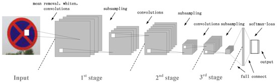
Figure 1. Network structure diagram.

3.1. Convolutional Layer

The convolutional layer is designed to extract features and it depends on the convolution operation. The convolution operation is basic to image processing, and most feature extraction methods use convolution operations to get the features. For example, images are filtered by various edge detection operators to get the edge features. The image feature is a kind of relationship between the pixel and its neighborhood pixels. The target features are obtained by convolving the weights of the neighborhood pixels. In the convolutional layer of the CNNs, the inMap is first to be filtered by the learned kernels, then to be mapped by the activation function to generate the outMaps. The inMap is the input mapping of a certain layer, and the outMap is the corresponding feature map from this layer.

Suppose the $i^{th}$ inMap in $l^{th}$ layer is $x_i^{l-1}$ and the $i^{th}$ outMap in $l^{th}$ layer is $x_i^l$, we can define the convolution in $l^{th}$ layer:

$$x_i^l=g\left({\displaystyle \sum _{j\in M_i}{x_j^{l-1}}^{✼}{w}_{ji}^l}+b_i^l\right)$$

(1)

where $g$ is the activation function, $M_i$ is a selection of the $i^{th}$ inMaps, $w_{ji}^l$ is the related weight of $x_j^{l-1}$, and $b_i^l$ is the related offset of $x_j^{l-1}$. The activation function is used to add the nonlinear factor into the network for improving the representation capacity. There are two activation functions that usually appear in neural networks. One is the sigmoid function, and another is the tanh function. As the standard logistic sigmoid, they are equal to a linear transformation and both stimulate the work of neurons [28]. For reducing the network computational burden, the rectifier activation function (ReLU) $f\left(x\right)=\max \left(0,x\right)$ is applied to reserve effective features and reduce some data redundancy. Some outputs of neurons are set to 0 by this function, which makes the network obtain sparse representations. Moreover, ReLU reduces the dependence between parameters, thus reducing the occurrence probability of over-fitting. Therefore, we choose ReLU as the activation function.

3.2. Subsampling Layer

Each convolutional layer is followed by a subsampling layer in every stage. If the feature maps are directly used as the feature vectors to train the classifier, it will create a huge challenge to deal with the computational complexity. In order to solve this problem, the feature dimension can be reduced by subsampling the features. Subsampling is realized by pooling features over a local area, therefore it is also called pooling in the CNNs. Pooling possesses invariance to small transformations of the input images [27], which leads it to find wide application in visual recognition.

Max pooling, average pooling and spatial pyramid pooling are the typical methods. Max pooling selects the maximum value of the local area, and average pooling obtains the mean value of the local area. Spatial pyramid pooling can transfer images with different size into feature vectors with the same dimensions, and it mainly solves the multiscale problem [29]. The parameter errors from the convolution layer can result in an offset of the estimated mean over the image [30]. Max pooling is effective for minimizing the impact on the average and retains more texture information. Otherwise, the limited local area size leads to the increase of the variance of estimation values. Average pooling can decrease the growth and retain more image background. To make full use of max pooling and average pooling, they are both utilized in our network.

3.3. Full-Connected Layer & Softmax-Loss Layer

After the three stages for feature extraction, two full-connected layers connect these feature maps with the final feature vectors. The first full-connected layer is identical to a convolutional layer. The input image is mapped onto feature maps with many pixels in the traditional convolutional layer, but the full-connected layer maps the input image onto a pixel by means of the convolution operation. This layer is aimed at reducing the dimension and prepares for the classification. The second full-connected layer is similar to a Single-hidden Layer Feedforward Neural Network (SLFN), and the output size is equal to the class number.

The last layer is usually a softmax layer in CNNs. We adopt the softmax-loss as the classifier layer, because it provides a more numerically stable gradient. The softmax-loss layer is equivalent to a softmax layer followed by a multinomial logistic loss layer [31]. The softmax function can be defined as

$$P\left(inMap\in i^{th}|inMap\right)=\frac{{\mathrm{e}}^{{inMap}_i}}{{\displaystyle \sum _{j=1}^{\mathrm{{\rm N}}}{\mathrm{e}}^{{inMap}_j}}},i=1,\mathrm{...},\mathrm{{\rm N}}$$

(2)

where P is the softmax probability of the i^th class, the ${inMap}_{\mathrm{j}}$ is the j^th element of the input vector inMap, and N is the class number. If the inMap belongs to the i^th class, the probability P will be 1, otherwise be 0.

The softmax-loss function combines the softmax function with the negative log-likelihood function, which aims to maximize the softmax probability. The representation of multinomial logistic loss is equivalent to the negative log-likelihood function, and it can be expressed as

$$\ell \left(i,P\right)=-\ln \left(P\right)$$

(3)

Thus, the softmax-loss function is defined as

$$\ell \left(i,inMap\right)=-\ln \left(\frac{{\mathrm{e}}^{{inMap}_i}}{{\displaystyle \sum _{j=1}^{\mathrm{{\rm N}}}{\mathrm{e}}^{{inMap}_j}}}\right)=\ln \left({\displaystyle \sum _{j=1}^{\mathrm{{\rm N}}}{\mathrm{e}}^{{inMap}_j}}\right)-{inMap}_i$$

(4)

In the function, there are only two inputs. One is the true label $i$ from the data layer at the bottom, and the other is the inMap from the full-connected layer. The data layer remains invariant when we train the network, and the inMap’s partial derivative is used to learn backpropagation. In the test phase, the test result relies on the position of the maximum probability.

3.4. Overall Architecture

In this section, we will introduce the overall architecture of our network. As shown in Table 1, the whole network contains 10 layers. The 6 layers following the input layer can be divided into three stages with the similar basic composition. The remaining three are two full-connected layers and a softmax-loss layer. The first full-connected layer is expressed as a convolutional layer. The output of the last full-connected layer is fed to a 43-way linear layer with softmax-loss which predicts the 43 class labels.

Table 1. The Inception architecture of our network.

Layer	Type	Number of Maps and Neurons	Kernel Size	Stride	Pad
1	input	3 maps of 32 × 32 neurons	-	-	-
2	Convolutional ReLU	32 maps of 32 × 32 neurons 32 maps of 32 × 32 neurons	5 × 5 -	1 -	2 0
3	average-pooling	32 maps of 16 × 16 neurons	3 × 3	2	[0 1 0 1]
4	Convolutional ReLU	32 maps of 16 × 16 neurons 32 maps of 16 × 16 neurons	5 × 5 -	1 -	2 0
5	average-pooling	32 maps of 8 × 8 neurons	3 × 3	2	[0 1 0 1]
6	Convolutional ReLU	64 maps of 8 × 8 neurons 64 maps of 8 × 8 neurons	5 × 5 -	1 -	2 0
7	max-pooling	64 maps of 4 × 4 neurons	3 × 3	2	[0 1 0 1]
8	Convolutional ReLU	64 maps of 1 × 1 neurons 64 maps of 1 × 1 neurons	4 × 4 -	1 -	0 0
9	full-connected	64 maps of 1 × 1 neurons	1 × 1	1	0
10	softmax-loss	43 neurons	-	-	-

Our network maximizes the multinomial logistic regression objective, which means that the network parameters can be tuned to minimize the average across training cases of the log-probability between the correct label distribution and the prediction. We train this network using the stochastic gradient descent with a batch size of 100 examples, momentum of 0.9, and weight decay of 0.0001. The update rule is the same as the AlexNet [21].

The input images have the equal size of 32 × 32 × 3. The first stage contains a convolutional layer and an average-pooling layer. The convolution layer firstly performs 32 convolutions in parallel to produce a set of linear activations. The input image padded with zeros by 2 pixels is filtered by 32 kernels of size 5 × 5 with a stride of 1 pixel. The size relationship between inMap and outMap in the convolutional layer can be expressed as

$${size}_{out}=\frac{{size}_{in}+p^2-{size}_{kernel}+1}{s}$$

(5)

where ${size}_{in}$, ${size}_{out}$, ${size}_{kernel}$ are the width or height of the inMap, outMap, and filter, p is the pixel number of padding, and s is the pixel number of stride. As a result, the size of outMap of the first convolutional layer is 32 × 32. Then, each linear activation runs through the nonlinear activation function ReLU. The output size and the map number of the nonlinear mapping retain unchanged. The output size of the average-pooling layer is 16 × 16 after down-sampling. We set the kernel size of the average-pooling layer and the max-pooling to 3 as a default, and fix the stride to 2 to prevent the speed of subsampling being too fast. The padding values on the top, bottom, left, and right respectively are 0, 1, 0, 1.

The following two stages work on the same principle, except that the average-pooling is replaced by the max-pooling in the third stage. And the input number of maps becomes 64 in the third subsampling layer. The full-connected layers have 64 units each and the first utilizes the rectified linear activation ReLU to speed up the learning. The full-connected layers are responsible for combining the outputs of the last layer into a feature vector with a 64-way feature vector. Finally, a 43-way linear layer with softmax-loss is chosen as the classifier.

4. Experiments

We use the MatConvNet toolbox [32] to train our network. The initial weights are drawn from a uniform random distribution in the range [−0.05, 0.05]. Our experiments are conducted on a Core i7-6700K CPU (4.0 GHz), 16GB DDR3. In this section, we will introduce the experiments and the results.

4.1. Dataset

GTSRB is an internationally recognized traffic sign dataset, which contains more than 50,000 images. The image size ranges from 15 × 15 to 250 × 250 and the images are not all squared. The dataset is divided into 43 classes, and the similar classes are merged into 6 subsets depicted as Figure 2, respectively as speed limit signs, danger signs, mandatory signs, derestriction signs, unique signs and other prohibitory signs. Considering the effect of illumination changes, partial occlusions, rotations, weather conditions, the dataset is taken from the real-word environment. Since the GTSRB was held at IJCNN 2011, this dataset has been a standard and popular dataset for research on traffic sign recognition. The dataset provides location of region of interest (ROI) to remove the margin for reducing the disturbance of complex background. However, we only use the function $imresize\left(\right)$ in MATLAB to rescale all images to the unique size of 32 × 32 without removing the disturbed margin. The bicubic interpolation method is used in the process of resizing.

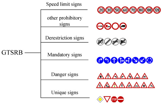
Figure 2. Subsets of traffic signs.

4.2. Experimental Analysis

The traffic sign images should be removed its mean activity from each pixel to ensure illuminant invariance to a certain extent. This preprocessing performs well as the normalization layer described in paper [21,24]. The normalization layer can implement a form of lateral inhibition inspired by the type found in real neurons, which is verified by competitive experiments [21]. Figure 3 shows that the preprocessing outperforms the method with normalization layer following the convolutional layer. The loss is the average of the output of the softmax-loss layer on the sample number, and the error rate is the percentage of the incorrectly-identified number to the total number. Figure 3a shows the loss of objective function changes with the increase of training epoch in logarithmic coordinates. Though the error curves in Figure 3b are close to each other, the curve without normalization layer has better convergence. After normalizing each image, the entire dataset should be whitened. In Figure 4, we randomly choose 20% of the traffic signs to show the effect of training with and without whitening. The plot shows a sharper downward trend in performance with whitening than without whitening. At the beginning of training, we suffer a loss of 15% or more accuracy. We lose at least 10% accuracy at the end. The results indicate that we will obtain better performance by incorporating whitening.

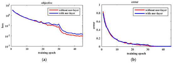
Figure 3. The effect of normalization layer. (a) The loss curve; (b) The error curve.

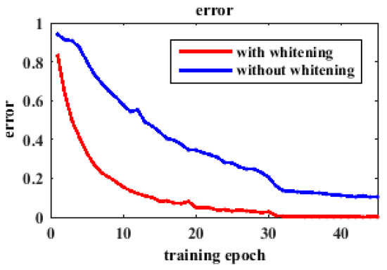
Figure 4. The effect of whitening.

The differences among the network-based CNNs lie in the realization of convolutional and subsampling layers and the training method. The selection of pooling method in each subsampling layer affects the recognition accuracy. Figure 5 clearly shows the effect of the combination of pooling. We have eight combinations: max-max-max, max-average-max, max-max-average, max-average-average, average-average-average, average-max-average, average-average-max, and average-max-max. The acronym of combination is used to represent each combination in Figure 5. We present the changes of loss and error rate with the increase of training epoch. The details are given to the right of the complete figure. The loss curves all appear to decrease and then maintain stable, which means the network converges on a certain range. Among these curves, the average-average-max in red presents faster convergence speed and smaller convergence value. In addition, average-average-max achieves the lowest error rate and shows a good classification ability in Figure 5b. The activation function ReLU in the first full-connected layer can speed up learning, so we compare the training speed with ReLU and without ReLU on the full dataset as depicted in Figure 6. The speed represents the training number per second. The full-connected layer removing the ReLU shows slower speed, which proves the ReLU has advantage of reducing the calculation time.

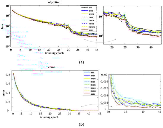
Figure 5. The effect of combination of pooling. (a) The loss curve; (b) The error curve.

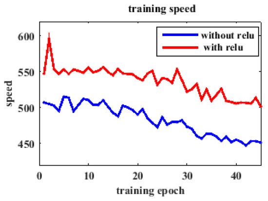
Figure 6. The effect of ReLU.

Therefore, we preprocess the input images in the following experiment, and choose the average-average-max pooling method.

The features are learned layer by layer. According to the back-propagation algorithm, the weights are tuned epoch by epoch to obtain robust features. We plot some weights from the first and second convolutional layers in Figure 7. For better visual effect, we enhance the figure contrast. As depicted in Figure 7a, every displayed filter is the superposition of the 3 filters connected to the red, green and blue channel of the input image respectively. The colorful filters convert the colorful input images into gray mappings. Therefore, every filter learned from the second layer is gray like Figure 7b, as well as the third layer. We also show the outMaps of each convolutional layer and subsampling layer in Figure 8. The pixel whose value is 1 appears white while the pixel whose value is 0 appears black. The feature maps become more and more abstract from one layer to the next. The size of the outMaps is reduced and the number is increased.

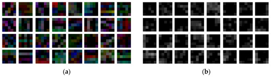
Figure 7. The learned filters of the first convolutional layer and the second. (a) The filters of the first convolutional layer; (b) The filters of the second convolutional layer.

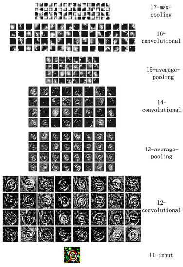
Figure 8. The outMaps from layer-1 to layer-7.

We compare the proposed network with traditional hand-crafted methods and networks based CNNs. These methods are listed as follows.

• HOGv+KELM [15]: It proposes a new method combing the ELM algorithm and the HOGv feature. The features are learned by the HOGv, with improvements compared with the HOG.
• SHOG5-SBRP2 [16]: It proposes a compact yet discriminative SHOG descriptor, and chooses two sparse analytical non-linear classifiers for classification.
• Complementary Features [17]: The extracted 6252-D features are 2560-D HOG feature, 1568-D Gabor filter feature and 2124-D LBP feature.
• HOS-LDA [18]: It extracts the features by HOS-based entropies and textures, and maximizes between class covariance and minimizes within class covariance through LDA.
• Multi-scale CNNs [24]: The output of every stage of automatically learning hierarchies of invariant features is fed to the classifier. Features are learned in these CNNs.
• Committee of CNNs [23]: It is a collection of CNNs in which a single CNN has seven hidden layers. Features are learned in these CNNs.
• Human (best individual) [33]: Eight test persons were confronted with a randomly selected, but fixed subset of 500 images of the validation set. The best-performing one was selected to classify the test set.
• Ensemble CNNs [25]: It proposes a hinge-loss stochastic gradient descent method to train CNNs. Features are learned in these CNNs.
• CNN+ELM [26]: It takes the CNNs as the feature extractor while removing the full-connected layer after training. The ELM is chosen as the classifier. Features are learned in these CNNs.

Table 2 shows the recognition rate of six algorithms on the 6 subsets. As a whole, the methods based on CNNs perform better than traditional hand-crafted methods. The committee of CNNs and our method even outperform the human performance, showing that deep learning has a powerful learning ability. The best individual results are presented in bold. The HOGv+KELM can accurately identify other prohibitory signs, mandatory signs, and unique signs. It is an effective one among the traditional algorithms for good feature representation. Human performance has an advantage over others on several subsets, but the limit on human sight causes humans to not be able to recognize signs with severe deformation. Though our method is not the best for recognizing each subset, it shows a stable performance. The most difficult class for all algorithms are danger signs, because this subset contains many images at low resolution. Image resolution is an important factor for image recognition.

Table 2. Individual results (%) for subsets of traffic signs.

	Speed Limits	Other Prohibitions	Derestr-iction	Mandatory	Danger	Unique
HOGv+KELM [15]	99.54	100	98.33	99.94	98.96	99.95
Complementary Features [17]	98.56	99.73	92.50	99.55	97.31	99.90
Multi-Scale CNNs [24]	98.61	99.87	94.44	97.18	98.03	98.63
Committee of CNNs [23]	99.47	99.93	99.72	99.89	99.07	99.22
Human (Best Individual) [33]	98.32	99.87	98.89	100	99.21	100
Our Method	99.93	99.80	99.44	100	99.13	99.90

Furthermore, a comparative experiment is conducted on the full GTSRB dataset. As shown in Table 3, our method leads to much improvement compared with the other methods. The best reported result at IJCNN 2011 was achieved by a committee of CNNs with an accuracy of 99.46%. The ensemble of CNNs achieves better performance than the committee of CNNs. Human performance is only at 98.84%, which is below several machine learning methods, indicating that the research on machine learning is meaningful for future development. The classification rates of traditional methods are much lower than the CNNs. According to the results, our method gives the best accuracy, at 99.84% for the complete dataset. This shows the robustness of the proposed network over the other methods.

Table 3. Comparison of accuracy (%) of the methods.

Method	Accuracy
Our method	99.84
Ensemble CNNs [25]	99.65
HOGv+KELM [15]	99.56
Committee of CNNs [23]	99.46
CNN+ELM [26]	99.40
Human (best individual) [33]	98.84
Complementary Features [17]	98.65
Multi-Scale CNN [24]	98.31
SHOG5-SBRP2 [16]	98.17
HOS-LDA [18]	97.84

In Table 4, we also list the training time and recognition time of several methods based on the CNNs. Though the computation platforms are different, we can still draw the conclusion that our method is more suitable for TSR. The networks depending on GPU not only increase the economy cost, but also need longer training time. Our network consumes less time and demands lower computation configuration, which makes our method more valuable in application.

Table 4. Comparison of training time and recognition time.

Method	Training Time	Recognition Time	Configuration
Our method	0.9 h/dataset	0.64 ms/frame	CPU: 8 × I7-6700K
Ensemble CNNs [25]	>7 h/dataset	N/A	CPU:I7-3960X GPU: 2 × Tesla C2075
Committee of CNNs [23]	37 h/dataset	11.5 ms/frame	CPU: I7-950 GPU: 4 × GTX580
CNN+ELM [26]	5 h/dataset	N/A	CPU: 8 × E5-2643

5. Conclusions

In this paper, we propose a shallow network for traffic signs recognition. Our network is composed of three stages for feature extraction, two full-connected layers, and a softmax-loss layer. In the stage of feature extraction, we combine max pooling and average pooling in subsampling layers. The shallow network learns discriminative features automatically and avoids the cumbersome computation of handcrafted features. The best recognition rate of our approach on the complete German traffic signs recognition benchmark dataset achieves 99.84% with lower time consumption. The results demonstrate that our method is applicable for traffic sign recognition in real-world environments. The disadvantage of our network is it requires a fixed input image size. Though Spatial Pyramid Pooling is a pooling method for images of arbitrary size, it is not suitable for small targets. Because the traffic sign recognition accuracy is poor by using the Spatial Pyramid Pooling. Therefore, the next work is to explore a method to break the restriction on image size while ensuring the recognition rate.

References

- Wollmer, M.; Blaschke, C.; Schindl, T. Online driver distraction detection using long short-term memory. IEEE Trans. Intell. Transp. Syst. 2011, 12, 574–582. [Google Scholar] [CrossRef]
- Qadri, M.T.; Asif, M. Automatic number plate recognition system for vehicle identification using optical character recognition. In Proceedings of the 2009 International Conference on Education Technology and Computer, Singapore, 17–20 April 2009; pp. 335–338. [Google Scholar]
- Wu, T.; Ranganathan, A. A practical system for road marking detection and recognition. In Proceedings of the 2012 International Conference on the Intelligent Vehicles Symposium (IV), Madrid, Spain, 3–7 June 2012; pp. 25–30. [Google Scholar]
- De la Escalera, A.; Armingol, J.M.; Mata, M. Traffic sign recognition and analysis for intelligent vehicles. Image Vis. Comput. 2003, 21, 247–258. [Google Scholar] [CrossRef]
- Fu, M.Y.; Huang, Y.S. A survey of traffic sign recognition. In Proceedings of the 2010 International Conference on Wavelet Analysis and Pattern Recognition, Qingdao, China, 11–14 July 2010; pp. 119–124. [Google Scholar]
- Gudigar, A.; Chokkadi, S.; Raghavendra, U.; Acharya, U.R. Multiple thresholding and subspace based approach for detection and recognition of traffic sign. Multimed. Tools Appl. 2016, 76, 1–19. [Google Scholar] [CrossRef]
- Geronimo, D.; Lopez, A.M.; Sappa, A.D. Survey of pedestrian detection for advanced driver assistance systems. IEEE Trans. Pattern Anal. Mach. Intell. 2010, 32, 1239–1258. [Google Scholar] [CrossRef] [PubMed]
- Mogelmose, A.; Trivedi, M.M.; Moeslund, T.B. Vision-based traffic sign detection and analysis for intelligent driver assistance systems: Perspectives and survey. IEEE Trans. Intell. Transp. Syst. 2012, 13, 1484–1497. [Google Scholar] [CrossRef]
- Gudigar, A.; Chokkadi, S.; Raghavendra, U. A review on automatic detection and recognition of traffic sign. Multimed. Tools Appl. 2016, 75, 333–364. [Google Scholar] [CrossRef]
- Liu, H.; Liu, Y.; Sun, F. Robust exemplar extraction using structured sparse coding. IEEE Trans. Neural Netw. Learn. Syst. 2015, 26, 1816–1821. [Google Scholar] [CrossRef] [PubMed]
- Lowe, D.G. Object recognition from local scale-invariant features. In Proceedings of the Seventh IEEE International Conference on Computer Vision, Kerkyra, Greece, 20–27 September 1999; pp. 1150–1157. [Google Scholar]
- Viola, P.; Jones, M. Rapid object detection using a boosted cascade of simple features. In Proceedings of the 2001 IEEE Computer Society Conference on Computer Vision and Pattern Recognition (CVPR), Hawaii, HI, USA, 8–14 December 2001; pp. 511–518. [Google Scholar]
- Liu, H.; Liu, Y.; Sun, F. Traffic sign recognition using group sparse coding. Inf. Sci. 2014, 266, 75–89. [Google Scholar] [CrossRef]
- Sun, Z.L.; Wang, H.; Lau, W.S. Application of BW-ELM model on traffic sign recognition. Neurocomputing 2014, 128, 153–159. [Google Scholar] [CrossRef]
- Huang, Z.; Yu, Y.; Gu, J. An efficient method for traffic sign recognition based on extreme learning machine. IEEE Trans. Cybern. 2016, 47, 920–933. [Google Scholar] [CrossRef] [PubMed]
- Kassani, P.H.; Teoh, A.B.J. A new sparse model for traffic sign classification using soft histogram of oriented gradients. Appl. Soft Comput. 2017, 52, 231–346. [Google Scholar] [CrossRef]
- Tang, S.; Huang, L.L. Traffic sign recognition using complementary features. In Proceedings of the 2013 2nd IAPR Asian Conference on Pattern Recognition, Okinawa, Japan, 5–8 November 2013; pp. 210–214. [Google Scholar]
- Gudigar, A.; Chokkadi, S.; Raghavendra, U. Local texture patterns for traffic sign recognition using higher order spectra. Pattern Recognit. Lett. 2017. [Google Scholar] [CrossRef]
- Lange, S.; Riedmiller, M. Deep auto-encoder neural networks in reinforcement learning. In Proceedings of the 2010 International Joint Conference on Neural Networks (IJCNN), Barcelona, Spain, 18–23 July 2010; pp. 1–8. [Google Scholar]
- Hinton, G.E. Deep belief networks. Scholarpedia 2009, 4, 5947. [Google Scholar] [CrossRef]
- Krizhevsky, A.; Sutskever, I.; Hinton, G. Imagenet classification with deep convolutional neural networks. In Proceedings of the Twenty-Sixth Annual Conference on Neural Information Processing Systems, Lake Tahoe, NV, USA, 3–8 December 2012; pp. 1097–1105. [Google Scholar]
- Lawrence, S.; Giles, C.L.; Tsoi, A.C. Face recognition: A convolutional neural-network approach. IEEE Trans. Neural Netw. 1997, 8, 98–113. [Google Scholar] [CrossRef] [PubMed]
- Cireşan, D.; Meier, U.; Masci, J. A committee of neural networks for traffic sign classification. In Proceedings of the 2011 International Joint Conference on Neural Networks (IJCNN), California, CA, USA, 31 July–5 August 2011; pp. 1918–1921. [Google Scholar]
- Sermanet, P.; LeCun, Y. Traffic sign recognition with multi-scale convolutional networks. In Proceedings of the 2011 International Joint Conference on Neural Networks (IJCNN), San Jose, CA, USA, 31 July–5 August 2011; pp. 2809–2813. [Google Scholar]
- Jin, J.; Fu, K.; Zhang, C. Traffic sign recognition with hinge loss trained convolutional neural networks. IEEE Trans. Intell. Transp. Syst. 2014, 15, 1991–2000. [Google Scholar] [CrossRef]
- Zeng, Y.; Xu, X.; Fang, Y. Traffic sign recognition using deep convolutional networks and extreme learning machine. In Proceedings of the International Conference on Intelligent Science and Big Data Engineering, Suzhou, China, 14–16 June 2015; pp. 272–280. [Google Scholar]
- Boureau, Y.L.; Ponce, J.; LeCun, Y. A theoretical analysis of feature pooling in visual recognition. In Proceedings of the 27th International Conference on Machine Learning (ICML-10), Haifa, Israel, 21–24 June 2010; pp. 111–118. [Google Scholar]
- Glorot, X.; Bordes, A.; Bengio, Y. Deep sparse rectifier neural networks. Aistats 2011, 15, 315–323. [Google Scholar]
- He, K.; Zhang, X.; Ren, S. Spatial pyramid pooling in deep convolutional networks for visual recognition. In Proceedings of the European Conference on Computer Vision, Zurich, Switzerland, 6–12 September 2014; pp. 346–361. [Google Scholar]
- Boureau, Y.L.; Bach, F.; LeCun, Y. Learning mid-level features for recognition. In Proceedings of the 2010 IEEE Conference on Computer Vision and Pattern Recognition (CVPR), New York, NY, USA, 13–18 June 2010; pp. 2559–2566. [Google Scholar]
- Szegedy, C.; Liu, W.; Jia, Y. Going deeper with convolutions. In Proceedings of the IEEE Conference on Computer Vision and Pattern Recognition, Boston, MA, USA, 7–12 July 2015; pp. 1–9. [Google Scholar]
- Vedaldi, A.; Lenc, K. Matconvnet: Convolutional neural networks for MATLAB. In Proceedings of the 23rd ACM International Conference on Multimedia, Brisbane, Australia, 26–30 October 2015; pp. 689–692. [Google Scholar]
- Stallkamp, J.; Schlipsing, M.; Salmen, J. Man vs. computer: Benchmarking machine learning algorithms for traffic sign recognition. Neural Netw. 2012, 32, 323–332. [Google Scholar] [CrossRef] [PubMed]
© 2017 by the authors. Licensee MDPI, Basel, Switzerland. This article is an open access article distributed under the terms and conditions of the Creative Commons Attribution (CC BY) license (http://creativecommons.org/licenses/by/4.0/).