Abstract
Verification of safety requirements is one important task during the development of safety critical systems. The increasing complexity of systems makes manual analysis almost impossible. This paper introduces a new methodology for formal verification of technical systems with smartIflow (State Machines for Automation of Reliability-related Tasks using Information FLOWs). smartIflow is a new modeling language that has been especially designed for the purpose of automating the safety analysis process in early product life cycle stages. It builds up on experience with existing approaches. As is common practice in current approaches, components are modeled as finite state machines. However, new concepts are introduced to describe component interactions. Events play a major role for internal interactions between components as well as for external (user) interactions. Our approach to the verification of formally specified safety requirements is a two-step method. First, an exhaustive simulation creates knowledge about a great variety of possible behaviors of the system, especially including reactions on suddenly occurring (possibly intermittent) faults. In the second step, safety requirements specified in CTL (Computation Tree Logic) are verified using model checking techniques, and counterexamples are generated if these are not satisfied. The practical applicability of this approach is demonstrated based on a Java implementation using a simple Two-Tank-Pump-Consumer system.
1. Introduction
During development of safety critical systems, several analysis tasks like FMEA (Failure Mode and Effects Analysis), FTA (Fault Tree Analysis) or CCA (Common Cause Analysis) are performed [1]. Besides that, safety engineers often verify the correctness of systems using safety requirement specifications. Performing this task manually can be time-consuming and error prone since every system reaction to failures or external inputs has to be predicted. In addition, it becomes more and more challenging as the complexity of system design steadily grows. Today, we find software in almost every technical system, and the rising number of interconnections between different systems makes it difficult to limit the scope of analysis.
There is obviously a need for automation. Existing approaches like Rodon [2], AltaRica [3], and HiP-HOPS [4] have already proven that reliable and useful safety analysis results can be obtained using formal models of the system. However, the success of fully automated approaches to safety analysis in an industrial context is still limited. One important aspect for the development of formal methods is balancing concurring goals, e.g., expressiveness of the modeling language and modeling costs, or detailed depth of analysis results and computational costs. New design decisions with respect to these trade-offs have the potential to increase the benefit/cost ratio in practical applications, and, by that increase, the attractiveness of formal approaches to automated safety analysis.
smartIflow (State Machines for Automation of Reliability-related Tasks using Information FLOWs) [5] is a new modeling language that has been specially designed for the purpose of automating the safety analysis process. It shares many features with existing approaches, especially AltaRica (though this was not our starting point), but some are new. The selected combination provides new answers to the trade-offs mentioned above.
This paper describes our approach to automated verification of technical systems with smartIflow. We discuss the modeling language in detail and compare it with existing approaches. The main objective is to automatically verify a safety specification against a system model. In this context, the following questions arise:
- How can such requirements be described in a formal language?
- How can the simulation be controlled to capture all relevant sequences of events?
- What might a verification result look like?
We will answer these questions by introducing our new verification method that is based on temporal formulas. It is being studied whether and how model checking techniques can be used.
This paper is organized as follows. The following section introduces some fundamental model checking concepts. In Section 3, existing approaches to model-based safety analysis are discussed. In Section 4, syntax and semantics of smartIflow are described, and differences to existing approaches are highlighted. In Section 5, the automated verification of safety requirements with smartIflow is discussed. The results of our experiments with a simple Two-Tank-Pump-Consumer system are shown in Section 6. Finally, a short summary concludes the paper.
2. Model Checking
Model Checking [6] describes the process of verifying a system model M against a specification ϕ. The objective is to prove whether M fulfills the specification ϕ. In other words: ? This verification is performed fully automatically. System models describe the possible system behaviors in a formal way. Finite state machines or transition systems are often used for behavioral description. The verification algorithm systematically explores all states and tries to disprove the specification. If the model does not fulfill the specification, the algorithm will deliver a counterexample, i.e., a trace of the system behavior that falsifies the property. However, most model checking tools like NuSMV deliver only one counterexample even though more could exist [7].
2.1. Linear Temporal Logic
Most model checking tools allow specifications to be expressed in temporal logics, like linear-time temporal logic (LTL) or Computation Tree Logic (CTL). LTL [8] allows for creating formulas about future paths. Consequently, besides the usual logical operators ( and ⇔) and operators for atomic expressions () there is also a set of temporal operators:
- : ϕ has to hold in the neXt state,
- : ϕ has to hold at each state of the subsequent path (Globally),
- : ϕ has to hold somewhere on the subsequent path (some Future state),
- : ψ has to hold Until ϕ holds,
- : ϕ has hold up to the moment when ψ becomes true (Release).
An example for the safety specification “Every occurrence of an event is eventually followed by an action” expressed in LTL might look like: G(event ⇒ F(action)).
2.2. Computation Tree Logic
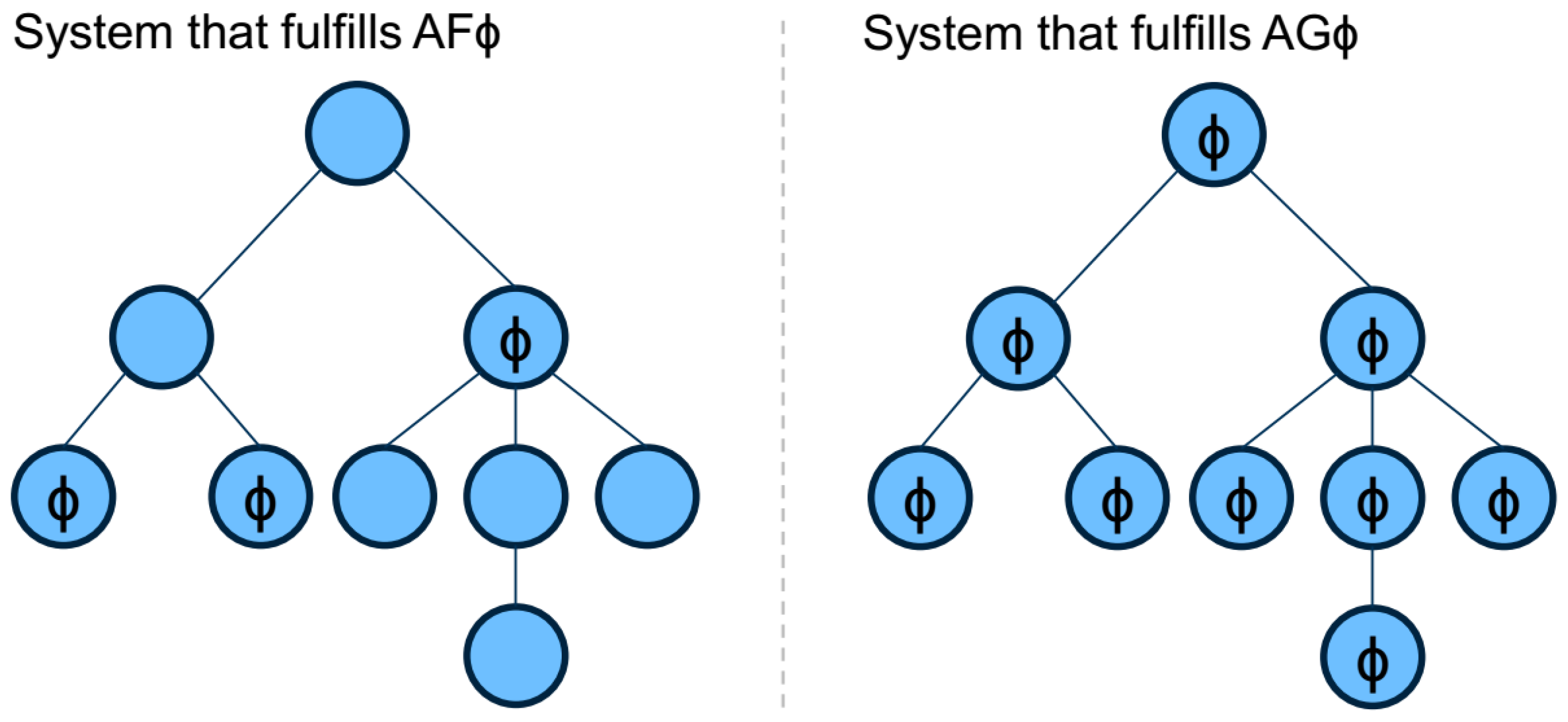
In contrast to LTL, CTL allows for creating statements about states of trees. Therefore, besides logical operators, CTL provides a set of temporal connectives. Each temporal connective is a pair of symbols. The first symbol specifies the path quantifier, which is either A (along All paths) or E (there Exists at least one path). The second symbol stands for a set of temporal operators, namely X (at the neXt state), F (at a Future state) and G (at all future states, i.e., Globally). The combination of these two symbols defines the most important operators (EX, EF, EG, AX AF and AG) to specify properties that take into account the non-deterministic behavior of a system. Consider the following property: “It is always possible to reach a safe state”. This may be expressed in CTL with the formula AF(EG(safe(s))). Figure 1 shows two example systems that fulfill or , respectively.
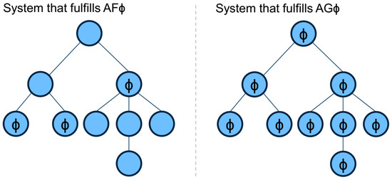
Figure 1.
Computation Tree Logic (CTL): Examples.
The expressiveness of LTL and CTL is quite different. Although there is an overlap, there are statements that can be expressed in CTL but not in LTL and vice versa. One should note that, for instance, NuSMV cannot generate counterexamples for all kind of CTL specifications [7].
3. Related Work
According to Lisagor et al. [9] and Batteux et al. [3], there are certain criteria that distinguish between different approaches to Model-Based Safety Analysis (MBSA). One criterion is the type of model construction. Basically, there are two approaches, namely extended system models (ESM) and standalone safety assessment models. As the name already implies, extended system models are system models (e.g., used for simulation) enriched with fault models. This method is also known as failure injection (FI). Standalone safety assessment models are models that are dedicated to safety-related tasks. This allows for incorporating only the knowledge that is actually needed for the analysis task, which reduces the overall complexity. Moreover, the specialized models allow for choosing an appropriate level of abstraction. This is very important since simulation models are often too detailed to get extensive information about system safety.
Another criterion is the semantics of the component interfaces. Essentially, there are two different approaches, namely failure logic modeling (FLM) and failure effect modeling (FEM). In failure logic modeling, each component is characterized by a set of component failures and a specification which describes how deviations in output values depend on deviations in input values and the current failure mode of the component. Modeling formalisms based on failure logic modeling only capture the occurrence, reaction and propagation of failures. Deviations are often limited to a set of predefined classes (e.g., commission or omission). As opposed to this, failure effect modeling uses the connections between components to share abstracted information about flow or energy. Failures on input signals or internal failures of a component are modeled by modifying the output signal. Obviously, failure effect modeling has a higher expressiveness than failure logic modeling, but, at the same time, the computational effort increases. There is also a hybrid approach using a combination of failure logic modeling and failure effect modeling.
Besides model construction and the semantics of component interfaces, there are two more important aspects. One aspect is the type of connection modeling. There are two fundamental types of connections, namely directed and undirected connections. Using directed connections often leads to problems in failure situations where the cause–effect relationship reverses. In modeling formalisms with directed connections, such situations can only be captured by creating additional connections between components, which increases model complexity and introduces gaps between model structure and reality. Especially if physical interactions play a significant role in system behavior, undirected connections and physical equation-based models have proven to be key to keep model structure close to reality. The last aspect in this list is the level of abstraction used for modeling systems. The level of abstraction of a modeling formalism has a quite high impact on both, the computational effort for analysis and the expressiveness of the results. Modeling formalisms using a high level of abstraction obviously will not deliver the same results as quantitative models (e.g., Simscape [10]). Quantitative models are useful to get detailed results. However, using them to get extensive information about the system behavior leads to extremely high computational effort and risks incomplete coverage of possible effects anyway due to the deterministic nature of detailed physical models.
There are many approaches to Model-Based Safety Assessment that can be found in literature, such as HiP-HOPS [4], Failure Propagation Transformation Notation (FPTN) [11], Rodon [2], deviation models [12], or the AltaRica language [3], to name only a few.
The AltaRica formalism follows the principle of standalone safety assessment models. Components in a system are represented by nodes. Each node consists of a set of flow and state variables, transitions, events, and equations to express the behavior. Flow variables are used to describe the component interfaces and to exchange information between components. AltaRica uses a combination of FEM and FLM (hybrid approach). Therefore, components may exchange information about failure modes as well as flow properties (e.g., energy) in an abstracted way. The AltaRica language has evolved over the years. In particular, the method of value propagation has been changed significantly. Although the last version of AltaRica [3] supports bidirectional flows, there are still no built-in elements to model physical flows. OpenAltaRica (http://openaltarica.fr/) is an integrated platform based on the AltaRica modeling formalism that provides a set of analysis tools. The abstraction level of AltaRica is quite high, but by no means as high as HiP-HOPS.
HiP-HOPS uses dedicated safety models, which utilize the structure of existing design models. The implementation is fully integrated into Simulink [13]. In HiP-HOPS, a component model is characterized by a set of logical expressions that specify the components reaction to internal failures or deviations at input ports. This formalism is based entirely on failure logic modeling since components only exchange information about signal deviations. The logical expressions are light-weight, cheap to create but quite limited with respect to expressiveness. There are no state variables to express state-dependent behavior, and connections between components are directional. HiP-HOPS models can be used to perform fault tree analysis (FTA) or failure modes and effects analysis (FMEA).
Joshi et al. [14] propose an approach based on Simulink and the NuSMV model checker. System models created in Simulink are enriched with a fault model by using failure effect modeling. These so-called extended system models are translated into the input language of the NuSMV model checker. In principle, Simulink is just used as alternative (graphical) representation for NuSMV models. A safety requirements specification created in CTL is used to verify the system behavior. If the system does not fulfill the specification, a counterexample with a trace of states that violated the specification is created. This approach also does not provide state variables, and connections are directional.
The SLIM (System Level Integrated Modeling Language) language was developed by the COMPASS (Correctness, Modeling project and Performance of Aero space Systems) project for modeling hardware and software systems for safety-related tasks [15]. Their framework supports several analysis methods, among others the generation of FMEA tables, fault tree analysis, and correctness verification. NuSMV is used as a fundamental platform for the various analysis tasks. System models in SLIM are translated into the input language of NuSMV, and temporal logic is used for requirement specification.
Another approach based on model checking has been introduced by Güdemann et al. [16]. System models are constructed in SAML (Safety Analysis and Modeling Language), which can be imported into several analysis tools like NuSMV or PRISM (Probabilistic Symbolic Model Checker).
This approach allows both qualitative and quantitative analysis.
Table 1 summarizes the key properties of existing approaches to MBSA. Obviously, the number of existing modeling formalisms, which support physical interactions between components, and are, at the same time, suitable for early stages of product development is not high. Only Rodon and AltaRica provide undirected connections. However, Rodon suffers from high computational costs, and the need of quantitative parameters and AltaRica’s capabilities to predict flows in non-trivial networks are limited.

Table 1.
Comparison of existing approaches to Model-Based Safety Analysis (MBSA).
4. The smartIflow Formalism
Based on the criteria discussed in the last section, smartIflow can be characterized as shown in Table 2.
Table 2.
Categorization of smartIflow according to criteria introduced in Section 3.
smartIflow shares with Rodon and AltaRica undirected connections, which helps to keep model and real structure in sync. Compared to Rodon, computational complexity (see e.g., [17]) is dramatically reduced by using finite domains only. This gives room for additional features like nondeterministic transitions, explicit events (as known from AltaRica, but here in a generalized form), and new component interaction concepts. In smartIflow, components communicate via ports and connections by manipulating and checking abstracted physical flows as well as by exchanging key-value-pairs that are called properties.
4.1. Fundamental Concepts
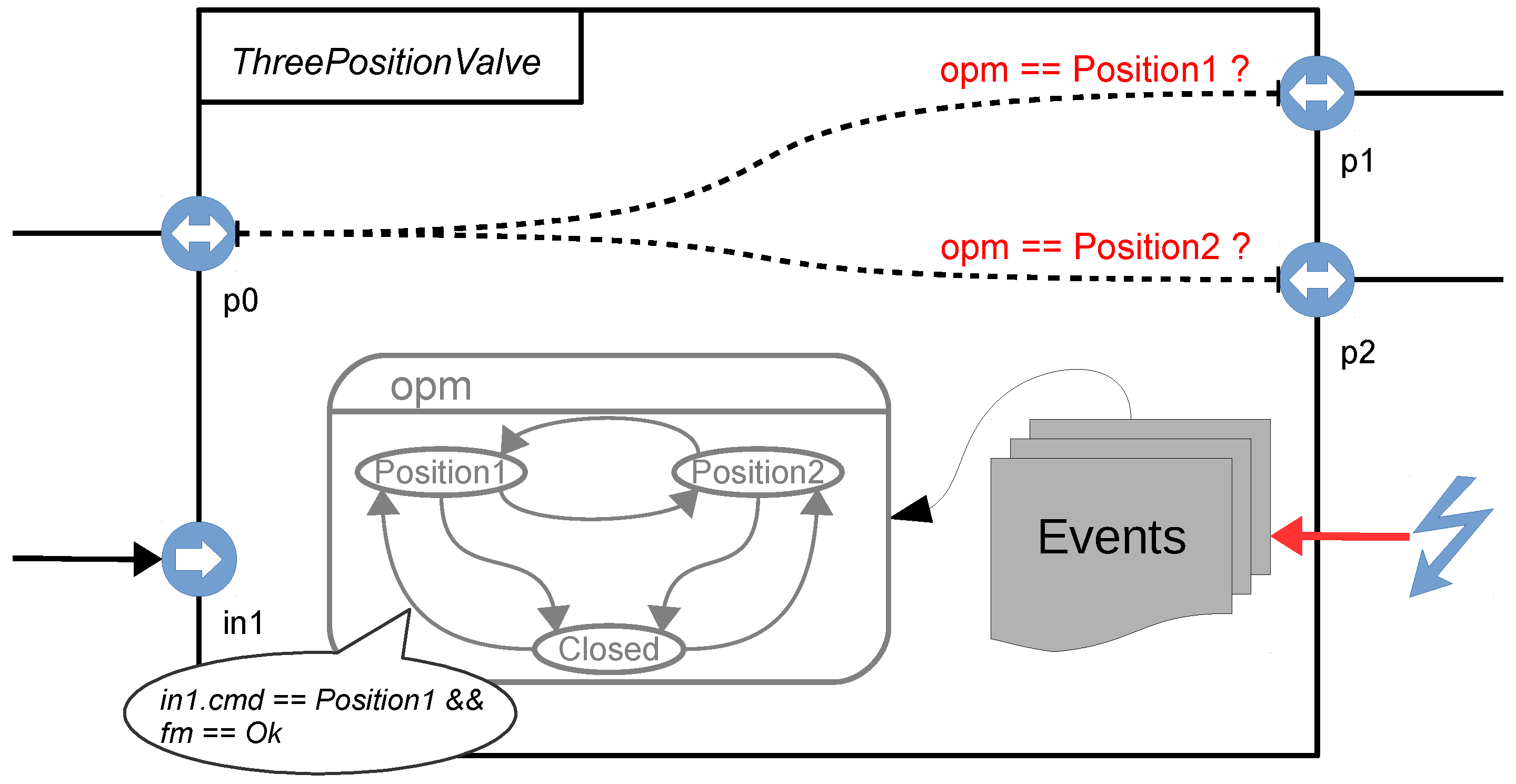
The smartIflow modeling language is component-based and object-oriented (though keyword extends is not yet implemented). Therefore, each component type in a system is characterized by a separate model class. Figure 2 visualizes the component model instance of a three-position valve.
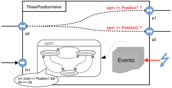
Figure 2.
Sketch of a smartIflow component.
Formally, a smartIflow component model instance is a tuple , where:
- C is a set of component instances (subcomponents). This allows for building hierarchical models.
- P is a set of ports. Ports represent the connection points of a component. Ports are typed (only ports with the same type can be connected) and can be marked as inputs or outputs (which affects property propagation). Components are linked through these ports.
- V is a set of state variables. Basically, each component in a system is considered as a finite state machine. Thus, a component consists of a set of state variables that are used to capture the operational and failure modes of a component. Each state variable is defined by a set of possible values (its domain) and also an initial value. State variables can only be accessed inside the component itself.
- E is a set of events. Events are used to stimulate a system externally, for example to change the operational mode of a component.
- B describes the state-dependent behavior of a component. The state-dependent behavior is described in terms of modifications to connection structure and also by adding properties to ports. Actually, properties are key-value pairs that provide a quite flexible mechanism to abstract from physical flow information. During simulation, properties are propagated through the connection structure. There are two types of connections: undirected channels for physical links and unidirectional channels for logical signals. Built-in primitives enable flow direction determination. The information about flow direction is available at each port by means of a reserved property (e.g., flow.dir = In).
- T describes the state transitions of a component. State changes are either performed after external events or after signal changes at ports initiated by other components (internal events). The condition of a state transition is a logical expression where propagated properties and state variables can be referenced. State transitions are positive edge triggered, which means that the transition is only performed when the result of a condition changes from to . Additionally, guard conditions are supported, as is usual in finite state machines.
Models in smartIflow can be composed graphically in Simulink/Simscape, as we described in a previous paper [18].
4.2. The smartIflow Language
Listing 1 shows an example of a component class definition in smartIflow.
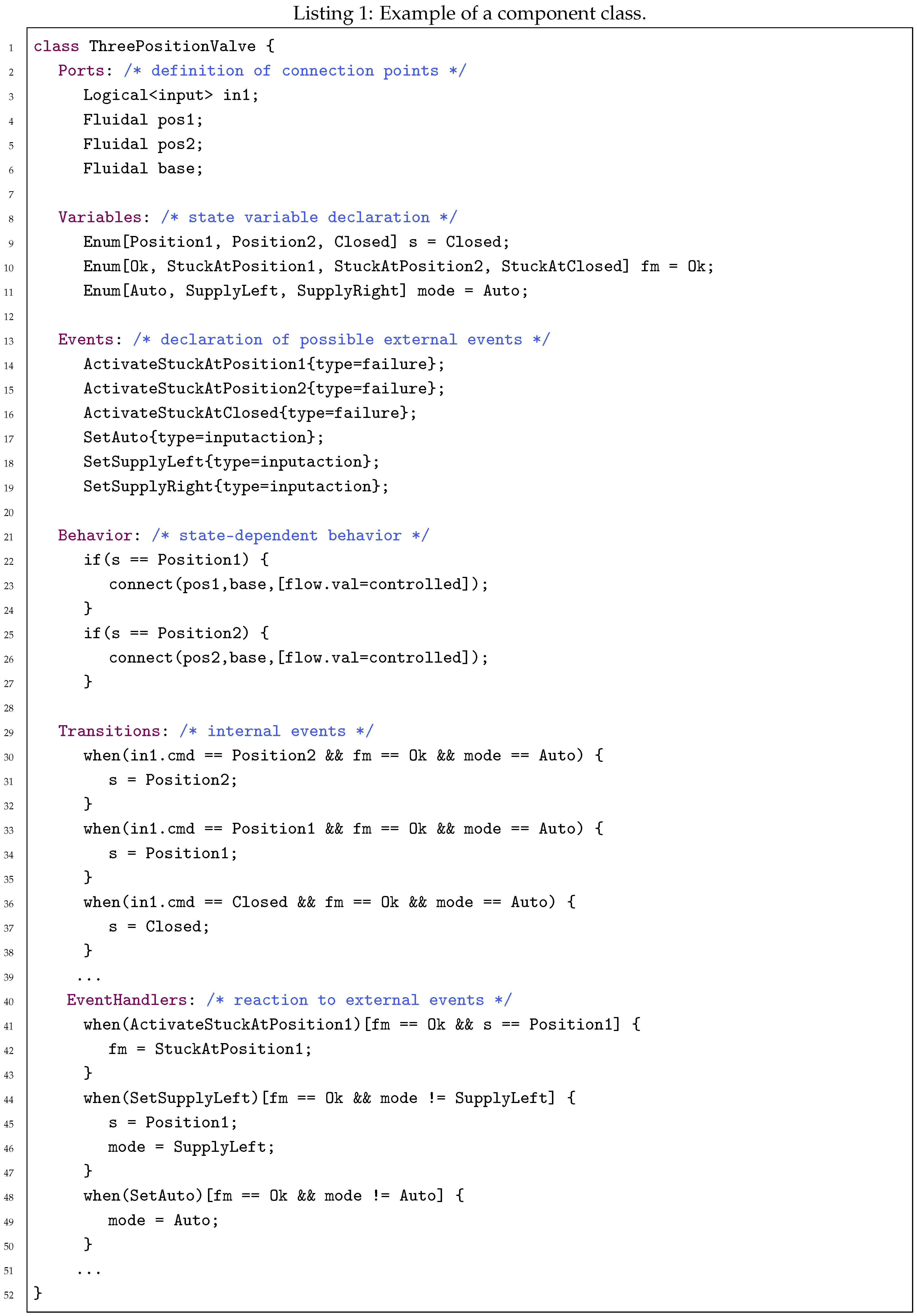
A class consists of a unique name and a sequence of sections. Each section describes a specific aspect of a component. The following sections can be used in a component class: Components, Ports, Variables, Events, Behavior, Transitions, and EventHandlers.
Section Components is used for component instantiation. Of course, each component instance must have a unique name. Section Ports is used to define the connectable ports of a component. For instance, the valve in our example has three ports of type Fluidal and one Logical<input> that is used for controlling the valve by command (Closed, Position1 or Position2).
State variables of a component are defined in the section Variables. The example class contains three state variables, namely s to describe the actual state of the valve, fm to describe the failure mode, and mode, which is necessary since the valve can also be controlled manually. Section Events is used to define external events. Optionally, events can be enriched with features that are indeed key-value pairs. Features can be used, for instance, to categorize events (e.g., group all failure events) or to assign a probability of occurrence. The latter is important for the calculation of the total failure probability.
Since the behavior of components is state-dependent, section Behavior consists of a set of conditional branches. Each conditional branch consists of a boolean expression and a set of actions. The boolean expression can be any logical combination of variable-value-equations. The actual behavior is described using set- and connect-actions. While set only publishes properties at a specific port, connect can be used to connect two ports. In addition, connect can publish a set of properties.
For state transitions, there are two sections, namely Transitions for internal events caused by signal changes initiated by other components, and EventHandlers for external events. Both sections consist of a set of when-clauses where the reaction to the events is specified. A when-clause consists of a condition, an optional guard, and assignments to state variables. A guard is a boolean expression that represents the precondition of a transition. The guard must be fulfilled in order to enable a transition.
5. Formal Verification of Safety Requirements with smartIflow
Basically, there are two types of model checking algorithms, namely symbolic model checking and explicit-state model checking. Symbolic approaches relay on transformations. As discussed in Section 3, NuSMV [7] is quite popular in the field of automated model-based safety analysis. It translates system descriptions into binary decision diagrams. Other approaches originating from the field of program verification reduce the problem to a satisfiability problem or a Horn constraint problem, which is then solved by an SAT (satisfiability) or constraint solver (see e.g., [19]). Symbolic approaches can handle very large state spaces, but the applicability is restricted to special types of system representations. Existing symbolic model checkers do not yet support complicated implicitly defined transitions including complex resistance network analysis steps. Another limitation of existing model checkers is the number of counterexamples provided in case the specification is disproved. Often, a certain system behavior cannot be guaranteed in every imaginable situation, but the likelihood for it can be optimized. In this case, counterexamples are of great interest, and it is not sufficient to deliver just one counterexample (as provided by e.g., NuSMV).
For this reason, we opted for the development of an explicit-state model checker. In our approach, the verification process is divided into two phases. First, the system behavior is simulated, and, in the second step, the specification is verified. This uncoupling has the great advantage that the verification does not depend on the simulation method. Conversely, various specifications can be checked without re-simulating the system. However, this two-phase approach may lead to larger search space exploration costs because simulation cannot profit from the safety requirement specification under verification. Both phases are now described in detail below.
5.1. Simulation
Algorithm 1 describes the simulation steps for behavior prediction. In our algorithm, a model state s consists of three components:
- vstate(s) describes the state of all state variables. It maps each variable to its current value.
- cstate(s) describes the truth value of all event conditions without guards of the parent state. It is a set and contains all fulfilled when-conditions from the Transitions and EventHandlers sections.
- pstate(s) describes the properties of all ports. Each port is mapped to the set of key-value pairs that are currently present at the port. When initializing a new state, each port is mapped to the empty set.
| Algorithm 1 The simulation algorithm |
|
States can be stable, which means that there is no transition that forces the system to move to another state. The model is expected to reach a stable state in every situation (the level of abstraction must be selected accordingly), and all external event triggers are limited to those stable states. Consequently, the dynamic model currently differentiates between two orders of magnitude of time-fast internal state transitions and slower external system stimuli.
After an initialization phase, where all state variables are set to their default value, the subsequent system states can be predicted. A single simulation step consists of four sub-steps. During the network reconfiguration, connections are created and properties are published depending on the values of the state variables. After that, flow directions are determined and properties are propagated. Thereafter, internal and external events are processed depending on the current state variable values and port properties. The result of this sub-step is a set of event-state pairs covering all possible subsequent states. For flow direction determination, different implementations are possible. The reference implementation uses a qualitative solver for order of magnitude (OM) resistance networks [20]. The two-step algorithm first reduces a network with one power source to a single equivalent resistor between the power source connection points by applying well known simplification techniques including e.g., star-polygon transformations. After that, the network is expanded and flow values are assigned at each level of expansion. This approach supports any power domain and multiple power sources. It works reliably for many supply network topologies. However, ambiguous flow results cannot always be avoided (e.g., for bridge circuits, qualitative resistance values are not always sufficient to estimate all flow directions precisely).
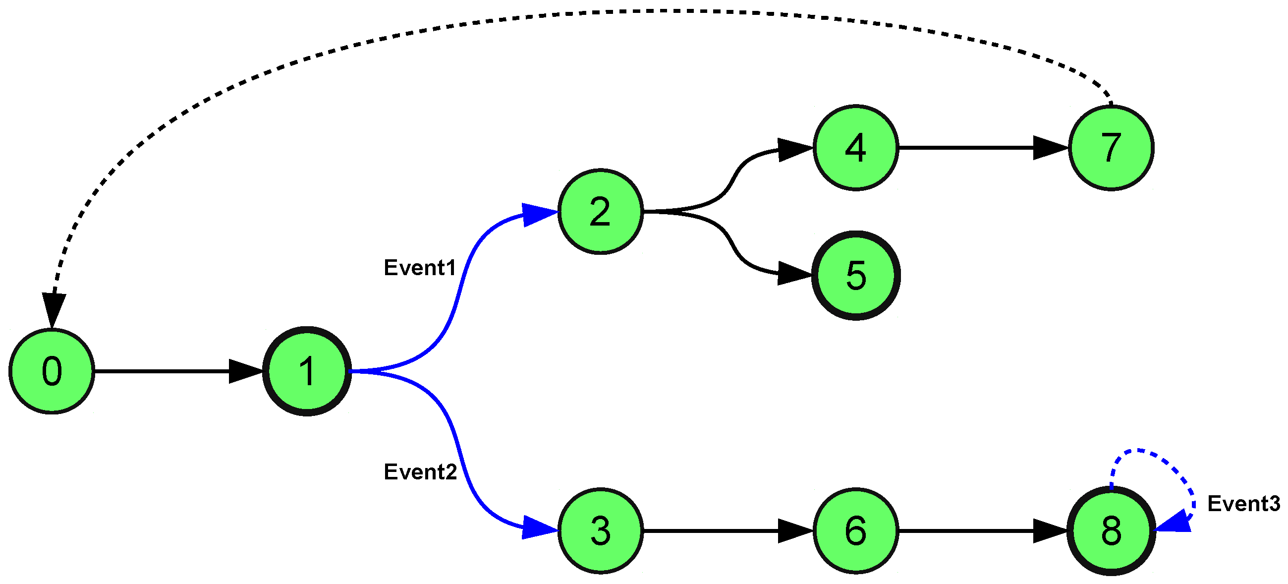
The simulation algorithm builds up a tree of nodes where the root node refers to the initial state, and children refer to successor states. To avoid repeated analyses of the same state, a lookup is used that maps already explored states to corresponding analysis nodes. If the lookup finds a successor, a reference is used instead of a parent–child relationship. Labels of child links and references indicate if the corresponding transitions were caused by external events.
Executing all possible combinations of events at each system state would lead to a state-space explosion. Moreover, it is unnecessary because there is a lot of constellations that cannot occur in reality (e.g., 20 components failing independently). In smartIflow, a formal event trigger specification language allows experts to express their knowledge about relevant event combinations on a path. For instance, events can be restricted to a special type, or the number of events of a specific type (e.g., failure events) can be limited. Due to space limitations, we cannot go into detail on the syntax and semantics of the language, but we will present concrete examples in the Section 6.
Figure 3 shows a possible outcome of behavior prediction.

Figure 3.
A possible simulation result.
5.2. Requirements Verification
The safety requirements need to be specified in a formal language. Typical safety requirements for a technical system might be:
- “It is always possible to reach a state within which some condition ϕ holds”.
- “After pressing button X, the system must react in a special way Y”.
In the case of the first requirement, LTL is not adequate since LTL can only express that a state in which ϕ holds is actually reached and not that it can be reached. As described in Section 2.1, LTL only allows to make specifications on a single path. CTL is able to formulate this property with formula . Therefore, we decided to use CTL. Specifications can be created using all usual CTL operators (). In atomic formulas, comparisons between all kind of variables, including propagated properties and symbolic values, can be expressed. Both properties at ports and variables can be accessed via the absolute path, starting at the root component (e.g., ).
The evaluation of expressions and subexpressions with a leading path quantifier is based on graph exploration. The exploration strategy depends on the operator Q. For instance, if the operator is , then the expression ϕ is verified at each node in all paths. ϕ can be any kind of expression, even an expression with a path quantifier. In that case, the evaluation of the expression does not begin at the root node of the simulation result, but rather at the current position of exploration. In the case of a violation of a CTL formula, a counterexample is generated. A counterexample is characterized by a trace of events that have been executed on the path from the root node to the node where the specification is violated. Unlike NuSMV, which only generates one counterexample, our approach is able to create all counterexamples that violate a specification. However, there are still CTL expressions that will not return any counterexample. For example, the expression will often result in just true or false. Even if the generation of counterexamples is possible for every sub-expression, there will not always exist a common counter example disproving both.
6. Example
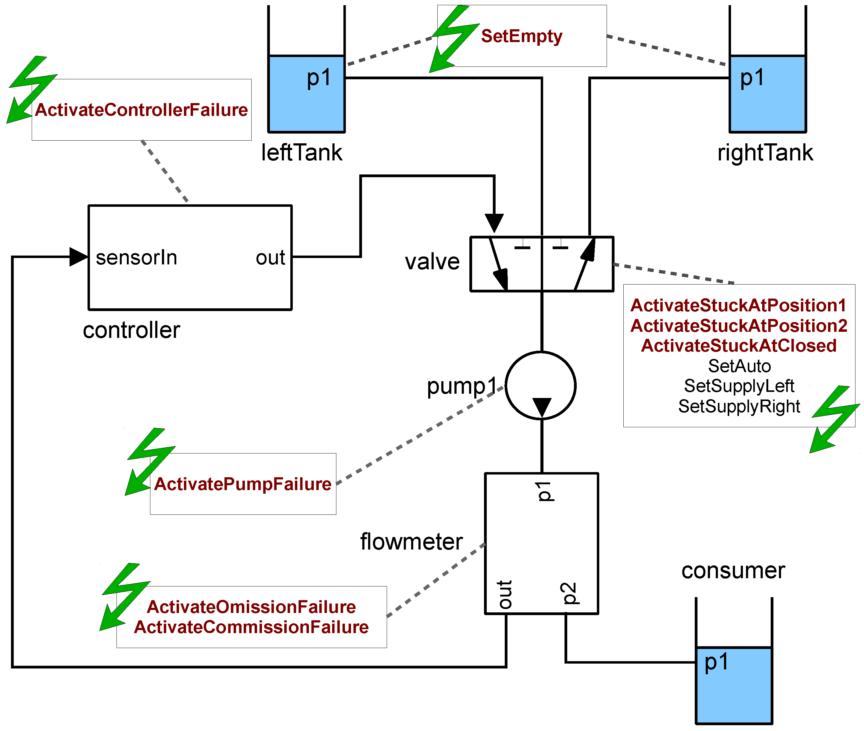
Figure 4 shows a very simple example system. The system consists of two tanks (leftTank, rightTank), a consumer which is modeled as a tank, a three-position valve, a flow meter, a pump, and a controller. The controller is responsible for keeping the consumer always supplied with liquid. In the case of an empty tank failure, the controller receives a zero-flow-message from the flow meter and solves the problem by sending a position change command to the valve. The valve can be controlled either by command or manually, using the external events SetSupplyLeft, SetSupplyRight, and SetAuto.

Figure 4.
Two-Tank-Pump-Consumer system.
In the first scenario, we check whether the system can guarantee liquid flow into the consumer without user interaction if the primary left tank is empty. The corresponding safety requirement in CTL is expressed by:
If we assume that scenarios with more than two independent failures are irrelevant, we can limit the search space using our event trigger specification language:
Verifying the above specification results in a set of counterexamples:
- If the pump is broken, there will not be any flow at all and consequently the consumer is not supplied with fluid.
- If the primary tank is empty and the valve is stuck at the first position (connected to the primary tank), the controller tries to switch to the secondary tank, which is obviously not possible. Consequently, the consumer is not supplied with fluid.
- A faulty flow meter delivers incorrect values to the controller. Therefore, the controller does not recognize the situation when the primary tank is empty.
- A defective controller does not respond to signal changes from the sensor. As a consequence, the system does not react to an empty tank.
In an extended scenario, we want to check whether a smart manual control of the valve can guarantee consumer supply in all cases where the automatic control failed. In order to enable user operations, the event trigger specification needs to be updated:
The updated safety requirement looks as follows:
This means that in case of an empty primary tank, there exists a path (a special manual control strategy) where the consumer is still supplied with fluid. Obviously, this property is not satisfied. Consequently, the verification algorithm delivers a set of counterexamples. The counterexamples show that the pump is a single point of failure. The consumer will no longer be supplied with liquid in case of a pump failure. A possible enhancement to the system for more robustness would be a second pump that is activated if the primary pump fails.
In our implementation, the smartIflow model of the Two-Tank-Pump-Consumer system consists of eight components. Table 3 shows some metrics obtained during simulation and verification.
Table 3.
Metrics of the Two-Tank-Pump-Consumer system.
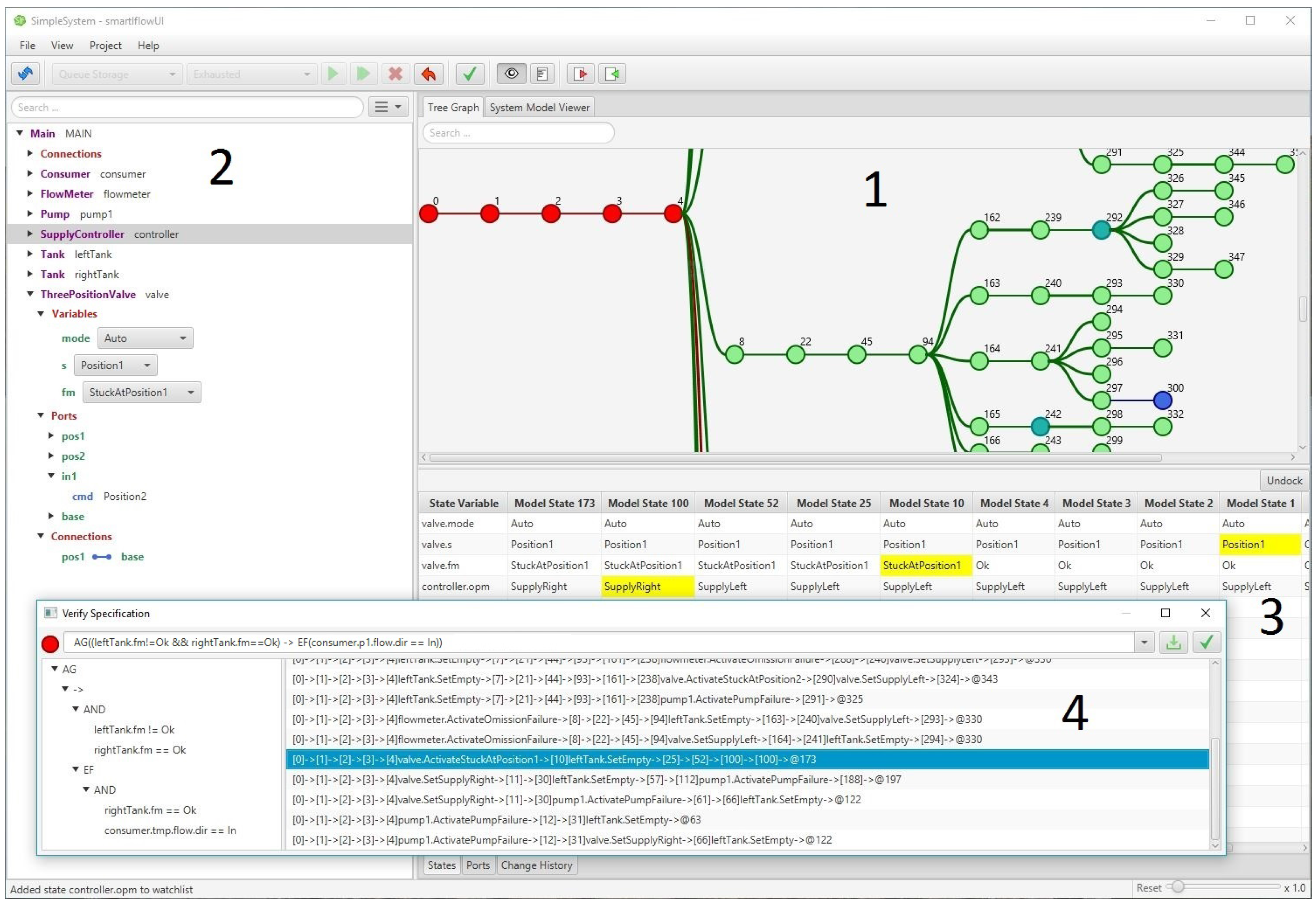
We have developed a tool that integrates the algorithms and provides an intuitive user interface for simulation tasks. Figure 5 shows our tool after simulation of the Two-Tank-Pump-Consumer system. The tree graph (1) visualizes the simulation result. Stable states (turquoise nodes), references to other nodes (blue nodes), and event transitions (bold lines) are highlighted to get a clear understanding about the system behavior. A selected node can be inspected with our model tree view (2). In this view, state variable values, properties at ports, and information about connections can be displayed. Since often only certain variables are of interest, our tool provides a watchlist (3) indicating the changes of certain variables on a selected path. The dialog for verification of safety requirements (4) allows specification of CTL formulas and displays the counterexamples in case of a violation. In addition, counterexamples are visualized in the tree graph by highlighting the state nodes that are part of the trace.
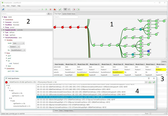
Figure 5.
smartIflow simulation tool.
7. Discussion
As current experience is based on models with limited size, there is still a long way to go to make this approach ready for application in an industrial context. It is not yet proven that the available controls are sufficient to keep search space under control. Understanding the massive data produced by simulation is another challenge, and extended views and analysis tools will be needed for this. Finally, there are many interesting options for extensions, e.g., computing minimal cut sets based on counterexamples resulting from CTL verification or adding component failure probabilities to the model to estimate probabilities of fatal system failures.
8. Conclusions
In this paper, we presented a new approach to model-based safety analysis. It is based on a new component-oriented modeling language that is specialized for safety analysis in early product development stages. Components are viewed as finite state machines, which is a common practice in many other existing approaches. The new modeling language differs from those approaches mainly in the way information is exchanged between the components. smartIflow supports non-causal modeling with bidirectional connections and abstracted physical flow determination on a qualitative level. A flexible property propagation mechanism supports message exchange between components. New messages can be added without the need to change types and add ports or connections. External events are supported as known from other languages like AltaRica. However, here, the concept is generalized for internal events that are triggered by signal changes based on positive edge semantics.
A methodology for formal verification of system design given a safety specification in CTL has been discussed as well. It is basically a model checking approach and uses tree-structured simulation data as input. The tree is created by exhaustive simulation. Expert knowledge from engineers is incorporated by means of a so-called event trigger specification to keep search space size under control. Since, in our model checker, the number of created counterexamples is not limited to just one (as common in other approaches), we believe that the obtained counterexample sets will prove to be useful for many other safety-related tasks, not only for disproving a specification.
The discussed concepts have been implemented and demonstrated using a simple Two-Tank-Pump-Consumer system as an example. The current tool chain includes an intelligent editor with syntax highlighting, a Matlab converter, and a simulation and verification environment with a graphical user interface (GUI). Although currently the size of analyzed models is limited, the obtained preliminary results seem very promising. Despite the abstract and light-weight character of the models, a wide range of aspects can be described adequately, especially physical flows, message exchange, and application logic.
Acknowledgments
We thank Christian Müller for his great work on the graphical part of the simulation tool. Special thanks go to the Institute for Applied Research (IAF) for funding his employment. We would also like to show our gratitude to Karin Lunde for proofreading this work and giving us many helpful comments. This research was supported by the Institute of Computer Science (IFI) of Ulm University of Applied Sciences.
Author Contributions
Rüdiger Lunde had the initial idea for the smartIflow project; the language in its current form has been developed together by Philipp Hönig and Rüdiger Lunde; Philipp Hönig did most of the implementation work, designed the Two-Tank-Pump-Consumer system, and performed the experiments; Philipp Hönig and Rüdiger Lunde wrote the paper; Florian Holzapfel contributed to this work with his application context knowledge; his feedback in regular meetings always encouraged the smartIflow team and influenced the direction of this work.
Conflicts of Interest
The authors declare no conflict of interest.
Abbreviations
The following abbreviations are used in this manuscript:
| CTL | Computation tree logic |
| FI | Failure injection |
| FLM | Failure logic modeling |
| FMEA | Failure mode and effects analysis |
| FSM | Finite state machine |
| FTA | Fault tree analysis |
| LTL | Linear temporal logic |
| MBSA | Model-Based Safety Analysis |
| smartIflow | State Machines for Automation of Reliability-related Tasks using Information FLOWs |
References
- Federal Aviation Administration (FAA). Chapter 9: Analysis Techniques. In FAA System Safety Handbook; Federal Aviation Administration: Washington, DC, USA, 2000. [Google Scholar]
- Lunde, K.; Lunde, R.; Münker, B. Model-Based Failure Analysis with RODON. In Proceedings of the 2006 Conference on ECAI 2006: 17th European Conference on Artificial Intelligence, Riva Del Garda, Italy, 29 August 29–1 September 2006; IOS Press: Amsterdam, The Netherlands, 2006; pp. 647–651. [Google Scholar]
- Batteux, M.; Prosvirnova, T.; Rauzy, A.; Kloul, L. The AltaRica 3.0 project for model-based safety assessment. In Proceedings of the 2013 11th IEEE International Conference on Industrial Informatics (INDIN), Bochum, Germany, 29–31 July 2013; pp. 741–746.
- Papadopoulos, Y.; McDermid, J.A. Hierarchically Performed Hazard Origin and Propagation Studies. In Computer Safety, Reliability and Security; Springer: Berlin/Heidelberg, Germany, 1999; pp. 139–152. [Google Scholar]
- Hönig, P.; Lunde, R. A New Modeling Approach for Automated Safety Analysis Based on Information Flows. In Proceedings of the 25th International Workshop on Principles of Diagnosis (DX14), Graz, Austria, 8–11 September 2014.
- Baier, C.; Katoen, J.P. Principles of Model Checking (Representation and Mind Series); The MIT Press: Cambridge, MA, USA, 2008. [Google Scholar]
- NuSMV 2.5 User Manual. Available online: http://nusmv.fbk.eu/NuSMV/userman/v25/nusmv.pdf (accessed on 29 December 2016).
- Huth, M.; Ryan, M. Logic in Computer Science: Modelling and Reasoning about Systems; Cambridge University Press: New York, NY, USA, 2004. [Google Scholar]
- Lisagor, O.; Kelly, T.; Niu, R. Model-based safety assessment: Review of the discipline and its challenges. In Proceedings of the 2011 9th International Conference on Reliability, Maintainability and Safety (ICRMS), Guiyang, China, 12–15 June 2011; pp. 625–632.
- Simscape. Available online: https://www.mathworks.com/products/simscape.html (accessed on 28 December 2016).
- Fenelon, P.; McDermid, J.; Nicholson, M.; Pumfrey, D. Towards Integrated Integrated Safety Analysis and Design. ACM Appl. Comput. Rev. 1994, 2, 21–32. [Google Scholar] [CrossRef]
- Struss, P.; Dobi, S. Automated Functional Safety Analysis of Vehicles Based on Qualitative Behavior Models and Spatial Representations. In Proceedings of the 24th International Workshop on Principles of Diagnosis (DX-2013), Jerusalem, Israel, 1–4 October 2013; pp. 85–91.
- Simulink. Available online: https://www.mathworks.com/products/simulink/ (accessed on 28 December 2016).
- Joshi, A.; Whalen, M.; Heimdahl, M.P. ModelBased Safety Analysis: Final Report; Technical Report; University of Minnesota: Minneapolis, MN, USA, 2005. [Google Scholar]
- Bozzano, M.; Cimatti, A.; Katoen, J.P.; Nguyen, V.Y.; Noll, T.; Roveri, M. The COMPASS Approach: Correctness, Modelling and Performability of Aerospace Systems. In Proceedings of the 28th International Conference on Computer Safety, Reliability, and Security, SAFECOMP 2009, Hamburg, Germany, 15–18 September 2009; Springer: Berlin/Heidelberg, Germany, 2009; pp. 173–186. [Google Scholar]
- Gudemann, M.; Ortmeier, F. A Framework for Qualitative and Quantitative Formal Model-Based Safety Analysis. In Proceedings of the 2010 IEEE 12th International Symposium on High-Assurance Systems Engineering (HASE), San Jose, CA, USA, 3–4 November 2010; pp. 132–141.
- Lunde, R. Towards Model-Based Engineering: A Constraint-Based Approach; Shaker: Aachen, Germany, 2006. [Google Scholar]
- Hönig, P.; Lunde, R.; Holzapfel, F. Modeling Technical Systems with smartIflow for Safety Related Tasks. In Proceedings of the International Workshop on Applications in Information Technology (IWAIT-2015), Aizu-Wakamatsu, Japan, 8–10 October 2015.
- Beyene, T.A.; Popeea, C.; Rybalchenko, A. Efficient CTL Verification via Horn Constraints Solving. In Proceedings of the 3rd Workshop on Horn Clauses for Verification and Synthesis, San Francisco, CA, USA, 3 April 2016.
- Snooke, N.A.; Lee, M.H. Qualitative Order of Magnitude Energy-Flow-Based Failure Modes and Effects Analysis. J. Artif. Intell. Res. 2013, 46, 413–447. [Google Scholar]
© 2017 by the authors. Licensee MDPI, Basel, Switzerland. This article is an open access article distributed under the terms and conditions of the Creative Commons Attribution (CC BY) license ( http://creativecommons.org/licenses/by/4.0/).