Article

The Information Content of Accounting Reports: An Information Theory Perspective

School of Management, State University of New York at Binghamton, Binghamton, NY 13902, USA
Information 2016, 7(3), 48; https://doi.org/10.3390/info7030048
Submission received: 26 March 2016 / Revised: 1 July 2016 / Accepted: 18 July 2016 / Published: 29 July 2016
(This article belongs to the Section Information Theory and Methodology)

Abstract

:
Is it possible to quantify the information content of accounting reports? If possible, then how? This study examines accounting as a classical communication system with the purpose of providing a framework with which to approach these fundamentally important questions. Information theory was established in the early-mid 20th century to describe the properties of classical communication systems. Applying concepts from this theory to an accounting context provides insight into the questions asked above. Specifically, a measure of the information content of financial statement numbers is developed from these information theory concepts. The measure is also applied to several large companies’ earnings numbers and aids in predicting their price movements.

1. Introduction

Does the financial accounting and reporting process provide non-redundant information to market participants? The over-arching goal of capital markets accounting research is to speak, in some way, to this question. The word “information”, and more pertinently, “accounting information”, appears repeatedly in the literature. However, we do not capture “information”, as defined according to classical information theory, with our stock price-based measure of the information content of accounting numbers.
The first half of the 20th century brought about a revolution in how humans think about information. Claude Shannon (the father of modern information theory) was at the forefront of this revolution. His landmark 1948 paper, A Mathematical Theory of Communication [1], was the first paper to formally describe a communication system in which information plays a central role. Concepts such as the capacity of an information channel, the uncertainty of a source and the optimal rate of information transmission in a noisy environment revolutionized how we think about information. These concepts laid the groundwork for much of the technology we appreciate today (e.g., the computer, cryptography, telecommunications, television, etc.). In the first paragraph of his landmark paper, Shannon describes the principal problem of communication; ironically, a problem not too distant from the purpose of financial accounting and reporting: The fundamental problem of communication is that of reproducing at one point, either exactly or approximately, a message selected at another point.
The purpose of this paper is to show why the long-standing criteria for deciding whether accounting numbers contain information does not logically reconcile with Shannon’s description of information in the context of a classical communication system. The financial accounting process can really be formalized as a classical communication system where information is determined to have been transmitted only when uncertainty regarding a future state-probability distribution has reduced. Consequently, I develop a measure of the information content of accounting reports based on Shannon’s entropy (uncertainty) measure introduced in 1948. The measure captures the information in an observed earnings realization (for example) as the percentage change uncertainty (relative to maximum) regarding which state earnings will be in the next period.

2. Related Research

A search of three of the top accounting journals over each of their respective lives found 341 articles in The Accounting Review, 210 in the Journal of Accounting Research and 99 in the Journal of Accounting and Economics in which the word “information” appeared in the title. Clearly, accounting researchers are interested in the concept of information and how to measure it.
These articles represent two streams of literature (one stream currently remains) that examine the information content of accounting numbers. Both streams borrow from information theory concepts originating with [1] and define information as the change in the state-probability distribution regarding a specific event (variable) upon transmission of a message from a source to a user (the extant stream hardly conceptualizes information explicitly this way anymore; rather, this idea is lurking implicitly in the background). What has differentiated these two streams is how each operationalizes the information content of an accounting message.
Theoretically, since accounting information falls under the realm of “information”, the definition given above is generalizable and maps well to an accounting context. The researcher quickly faces an immediate obstacle, however, when attempting to directly operationalize the definition. Specifically, how should the users’ ex ante (before the message is received) and ex post probability distributions be determined for a particular event or state of the world? These, of course, are not directly observable and, therefore, must be proxied.
The work in [2] was one of the first papers to examine the information content of accounting information; specifically, earnings. He states: The information content of earnings is an issue of obvious importance and is a focal point for measurement controversies in accounting. He looks at investors reaction to earnings announcements, as reflected in the volume and price movements of common stocks in the weeks surrounding the announcement date. He defines the information content of earnings as the degree of change in investors’ assessments of the probability distribution of future returns (or prices), where this change is proxied for by the degree of change in the equilibrium value of a company’s stock upon their announcement of earnings. This study laid the groundwork for a flurry of research (for example, see [3,4,5,6,7], to name a few), which uses the stock price reaction to a firm announcement as a proxy for the degree of change in investors’ assessments of the probability distribution of future returns and, hence, as a proxy for the information content of that particular announcement.
An important distinction is in order. The definition given above does not mention the word “uncertainty”. The definition is rather vague and does not tell us exactly what these investors’ “assessments of the probability distribution of future returns” are. In order for the above definition to reconcile with “information” as defined according to classical information theory, one must introduce the notion of uncertainty. Information is uncertainty reduction. Thus, the information content of earnings is the reduction in uncertainty regarding future earnings. Defined this way, however, the long-standing assumption that price equals discounted expected future earnings does not reconcile with this definition. Assuming price equals discounted expected future earnings implies that changes in price (returns) are equal to changes in discounted expected future earnings. As I discuss later, expected earnings do capture the various states that future earnings could take on, as well as the probabilities of those respective states, but do not capture changes in uncertainty regarding in which state that future earnings will be. Thus returns, viewed purely as a function of the change in discounted expected future earnings, do not capture changes in uncertainty and, hence, do not capture information. I show later that uncertainty regarding future earnings and that regarding expected future earnings are two different concepts. The first depends only on the state probabilities and the number of states and is independent of value. The second depends on the probabilities, the number of states and the value of earnings in each state. Given that information is uncertainty reduction, returns only capture information if one views price as a function of both uncertainty regarding future earnings and discounted expected future earnings.
Concurrent with Beaver’s idea regarding the information content of accounting numbers, a small stream of research surfaced whose intent was to try and capture investors state-probability distributions more directly. The work in [8] initiated interest in a communication theory approach to accounting information; pointing out that communication theory had been introduced in various other sciences, such as experimental psychology, linguistics and biophysics, but had not yet found its way into accounting. They state:
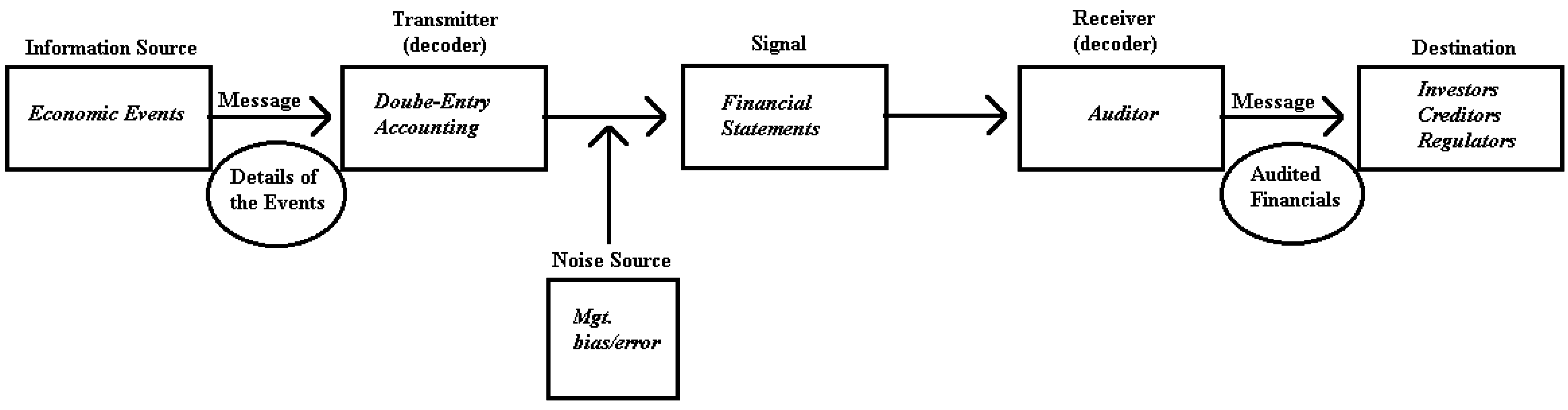
It seems reasonable to assume, however, that viewing accountancy as a communication process may provide a clearer picture of the nature and scope of the accounting function in an economic system. The opportunity exists because the underlying structure of communication theory may be used to describe the accounting process.
—Norton M. Bedford and Vahe Baladouni [8] (p. 650)
University of Chicago economist Henry Theil was the first to formally apply concepts borrowed from communication theory, specifically entropy, to an accounting context. The work in [9,10] applied Shannon’s information theory concept of entropy (uncertainty) (the functional form for entropy was originally proposed in physics by J. Willard Gibbs ([11]) to measure the amount of uncertainty in a particular set of particles (classical system)) to analyze the information content of financial statement items. He realized that every financial statement item can be expressed as some fraction of a total. For example, any particular type of asset can be expressed as a fraction of total assets. These fractions summed over all of the assets equal one by construction similar to an individuals’ state probability distribution. He then allowed these fractions, observed in period t, to proxy for an individuals’ ex ante t + 1 state probabilities (i.e., prior probabilities) for assets in period t + 1 . Once assets in period t + 1 were realized, he then allowed the observed t + 1 fractions to proxy for the individual posterior probabilities. He then could calculate the entropy attributed to the t + 1 asset realizations (message) and called this the information content of t + 1 assets.
Subsequent to this initial application of information theory concepts to accounting reports, [12,13] examined the information loss due to different levels of aggregation in the financial statements. He devised a measure of information loss as the change in entropy induced by varying the level of aggregation. As with Theil, the probabilities used in the entropy calculation were simply ratios of the various respective categories of assets (liabilities) to total assets (liabilities).
The idea of applying information theory in an accounting context is very appealing due to the theoretical similarity that an accounting system has with a communication system (see Figure 1 in the next section), and the above studies provide a reasonable approach along these lines.
This paper purposes to follow Shannon’s concepts as closely as possible to ensure that a theoretically correct application of communication theory to an accounting context is maintained. Along the way, a few, seemingly limiting, assumptions must be made to make things tractable. However, one should judge the measure developed in regards to its predictive ability; some evidence of which is provided in the empirical analysis.

3. Accounting as a Communication System

The general purpose of accounting is to communicate to interested users events that occurred in the past. We judge this communication to have been successful if these users are able, ex post, to “see” those events that transpired ex ante. To this end, we account for these events through time and at some point summarize this accounting by providing the user a set of summary reports.
As described above, accounting is simply a modified classical communication system. Such a system was the focus of Claude Shannon’s influential research and is depicted in Figure 1.
A communication system must begin with an information source that produces a message or sequence of messages to be communicated to an interested user. Economic events (I define economic events as transactions that are accounted for within the double-entry system. Of course, the accounting cannot capture the information in macro-level events, which are not felt at the firm level. To the extent that the firm-specific economic events are a function of the macro-level effects, this framework holds.) are the information source in an accounting context. These events transpire and give rise to the information that interested users demand. Next, a transmitter, or encoder, must be present to operate on the message in some way to produce a suitable signal for transmission. The double-entry system fulfills this purpose. This linear operator ensures that a record is maintained in at least two accounts for every economic event that transpires. There is some noise in this process, however, as Generally Accepted Accounting Principles (GAAP) are inherently subjective in their prescriptions. Furthermore, people are subject to error, as well. Thus, the double-entry system operates on the message in a noisy way; this noise being a function of managerial error, bias and/or subjective interpretation of GAAP. The output from the transmitter is the signal; an encoded version of the message. The financial statements (the statements themselves absent the footnotes) are the signal produced by the double-entry accounting system transmitter. The receiver, an auditor, receives the signal and decodes it. The goal of the decoding process is to try and recover the original message sent from the information source. The auditor performs a series of tests and procedures on the signal to ensure that it is as pure as possible. In a classical communication system, the receiver decodes the signal, recovers the original message with an arbitrarily small level of error and passes it on to its destination. In an accounting context, an auditor attempts to try and understand the original message from the signal, but cannot recover it fully. The auditor simply helps to make the signal a better depiction of the underlying message than it was previously. They act as a sort of filter on the signal. The filtering process intends to remove as much of the error and bias in the signal as possible. The auditor then passes the filtered signal on to its destination. The destination is the intended recipient of the original message sent from the information source through the transmitter. The destination in an accounting context would be investors, creditors, regulators and any other interested user of the financial statements. The analogy between a classical communication system and accounting breaks down at this last step as the destination does not receive the original message; rather, they receive a filtered signal that they must decode (audited financials).
Visualizing accounting with the framework described is a useful exercise as it helps us to realize that accounting is an example of a classical communication system. Of course, there are aspects of accounting that do not map well to the above framework, as pointed out above. Despite this fact, visualizing accounting with this framework enables us to more easily identify important questions regarding the accounting process. For example, we see that the transmitter fulfills an important role in the process, as it is the first stop the message makes towards the destination. The ability of the destination user to extract the original message depends first on certain properties of the transmitter. What are the important properties of a transmitter? It seems reasonable to require that it encode the message in such a way that accurate decoding is possible. That is, the function that encodes the message should have an inverse. If we perform the inverse operation of the transmitter, we should be able to recover the original message. Furthermore, it seems reasonable to require that the transmitter be self-correcting; self-correcting in the sense that, once a signal is observed, we can immediately tell if there is an error, absent any noise in the encoding process. Double-entry accounting does satisfy this property, as it ensures that the accounting equation is always in balance, unless an error has been made.
Another important question that arises from thinking about accounting as a communication system relates to the message itself. Is there a way to quantify the information content of the message that the destination user receives? Information theory was established as a way to analyze information content and other properties of classical communication systems. This seemed a natural progression, as telegraph, telephony, radio and television had all been invented prior to this time period.
Claude Shannon’s influential work in the 1940s described certain properties of classical communication systems mathematically and derived ways in which to ensure that these properties hold. He analyzed both noiseless and noisy communication systems and proved many results relating to the optimal encoding of messages in noisy environments. He proved for example that it is impossible to encode a message in such a way (data compression) that the probability of information loss is arbitrarily small (noise-less coding theorem). He also proved that, given a level of noise, it was possible to encode a message in such a way as to make the error in the resulting signal arbitrarily small (noisy coding theorem).
Arguably, Shannon’s most influential contribution, however, was his formulation of the uncertainty in a given message. His measure of uncertainty, information entropy, was the basis for much of his later work with communication systems (including the theorems above). Ironically, entropy as a measure of uncertainty already existed in physics at the time of his work; he just applied it in a classical communication system setting. He did not only apply it though. He proved his measure of uncertainty was the only function satisfying certain conditions one would intuitively expect such a measure to satisfy. This measure of uncertainty is the basis of the present paper, and in this measure lies one possible answer to the question boldedearlier. I expound on this in the next section.

4. Information Defined and Measured

Information is a rather elusive concept. As [14] point out, the concept of information is too broad to be captured completely by a single definition.
In this paper, I approach information from a probabilistic viewpoint and define information as follows (this definition is consistent with treatment of the term in [15]). Information—Knowledge, after which one receives and processes, that changes, in an uncertainty changing way, their ex ante probability distribution regarding a set of propositions or states. That is, information is a subset of knowledge and is defined in probabilistic terms. Knowledge that is “informative” will change the user’s probability distribution regarding a set of propositions or states in an uncertainty changing way. For example, if an individual received a forecast of tomorrow’s weather and the forecast reduced their uncertainty regarding which state the weather would be in (e.g., rainy or sunny), then the forecast was informative. This view of information being a change in uncertainty where uncertainty is a function of probabilities was most clearly first expressed in [1]. Given a probability distribution, P, for a set of possible states a particular variable could be in, Shannon showed that the following measure, U ( P ) , was the only measure of uncertainty that satisfied three intuitive criteria. (1) U ( P ) should be continuous in the state probabilities P. That is, small changes in P should produce small changes in U ( P ) . (2) U ( P ) should be maximized when all states are equally likely. (3) The uncertainty of a compound set of states S should be equal to a weighted average of the uncertainties of any particular mutually exclusive partitioning of S where the uncertainties of the partitions are weighted by their respective probabilities of occurrence.
U ( P ) = C i = 1 n p i * log ( p i )
where the constant C > 0 simply amounts to a choice of a unit of measure (for simplicity, and without loss of generality, I set C = 1 throughout the rest of this paper) and log ( p i ) is the base 2 logarithm of the i’-th state probability.

4.1. Information and Financial Accounting

The purpose of accounting is to record, and communicate to interested users, the effect of economic events or transactions on an entity. The details of these events are passed through the double-entry system and summarized in a signal commonly known as the financial statements. This signal is then operated on by a third, independent (supposedly “independent” in the case of the auditing firms) party, who filters out noise and error and then passes the signal on to the recipient (market participants) (see Figure 1). These recipients are assumed to be economically linked, in some way, to the entity and, therefore, have already formed ex ante probability distributions regarding the future states of the entity. Information therefore plays a central role in the financial accounting and reporting process. If the message (e.g., financial statements) does not change these users’ ex ante probability distributions regarding the future states of the entity, such that uncertainty changes, then the users are no better off after receiving and processing the message than they were before receiving the message. In this case, the user should be indifferent between these reports and a set of blank reports. Thus, information plays a critical role in helping one assess if the “accounting” that an entity does fulfilled its purpose. If it did not, then we are hard-pressed to find an economic benefit to offset the costs of doing the accounting.
Up to this point, I have introduced a framework that hopefully has persuaded the reader that a direct measure of the information content of a message would be greatly valued; particularly in an accounting context. From the definition, it seems logical to think in terms of measuring the change in uncertainty of the state-probability distribution. I formalize this concept in the next section.

4.2. A Measure of Information Content

Suppose an individual, which we will label a “user”, has a state-space in mind regarding some variable of interest (e.g., the “weather” in the example I gave previously), j, that may or may not affect a future decision. Denote the state-space as S j = { S ; P ( S | K I ) } where S = { s 1 , s 2 , , s n } is a discrete set of n states that the variable j can take on. P ( S | K I ) = P I = { α 1 I , α 2 I , , α n I } is a set of probabilities for each of these states assessed from knowledge possessed initially (that is, P ( S | K I ) is the ex ante, state-probability distribution for variable j) by the user. We assume S is exhaustive from the users’ standpoint, so that i = 1 n α i = 1 . That is, from the users’ standpoint, j must be in one of the states of S. Now, theoretically, j could be continuous and take on infinitely many states. The user, however, due to limited cognitive processing ability, does not view j as thus. She or he partitions the continuous variable j into a set of n states and attaches probabilities to those states. Furthermore, j cannot be in more than one state at a time, and I also assume that each of these n states is distinct (non-overlapping) (that is, s i s k = for all i , k ). Next, a message, M, is sent to the user from a source. Upon receipt of the message, the user processes the knowledge contained therein and updates his or her probability distribution to P ( S | K A ) = P A = { α 1 A , α 2 A , , α n A } . Based on the discussion in Section 4.1, let the information content of M, I C ( M ) , be defined as the scaled percentage change in the users’ uncertainty regarding the state-probability distribution P ( S | K ) as shown in Equation (2):
I C ( M ) = | U ( P I ) U ( P A ) | U ( P I ) if U ( P I ) > U ( P A ) | U ( P I ) U ( P A ) | log ( n ) U ( P I ) if U ( P I ) < U ( P A ) 0 if U ( P I ) = U ( P A )
where U ( P I ) and U ( P A ) are defined as in Equation (1). The function in Equation (2) measures the information content of a message in general. Now, I C ( M ) [ 0 , 1 ] and can be stated in percentage terms. This is possible due to the fact that U ( P ) = i = 1 n p i * log ( p i ) is bounded above by log ( n ) .
To visualize the measure I C ( M ) , consider the following. If we think of a continuum of uncertainty with zero at one end and log ( n ) at the other end, then both U ( P I ) and U ( P A ) lie on this continuum. If U ( P I ) > U ( P A ) , then uncertainty decreased upon receipt of the message. The information content of the message could be thought of as the percentage decrease relative to the maximum decrease that could be obtained. Conversely, if U ( P I ) < U ( P A ) , then uncertainty increased, and the information content of the message could be thought of as the percentage increase relative to the maximum increase that could be obtained. These scenarios are illustrated in Figure 2 and Figure 3.
In Figure 2, U ( P I ) < U ( P A ) ; thus, uncertainty increases by | a b | , and the maximum increase is log ( n ) a , where n is the number of states in the perceived state-space. Therefore, the information content of the message is | a b | log ( n ) a = | U ( P I ) U ( P A ) | log ( n ) U ( P I ) . In Figure 3, U ( P I ) > U ( P A ) ; thus, uncertainty decreases by | a b | , and the maximum decrease is a. Therefore, the information content of the message is | a b | a = | U ( P I ) U ( P A ) | U ( P I ) . Of course, when U ( P I ) = U ( P A ) , uncertainty does not change, and I assume that the information content of the message is zero (I discuss this assumption in more detail in the “Limitations” section). In the next section, I apply I C ( M ) , as given in Equation (2), to the quantitative financial statement information. Note that the measure introduced in Section 4.2 can measure the information content of any time series variable; not just those variables typically found in the financial statements.

5. Applying the Measure to Financial Statements

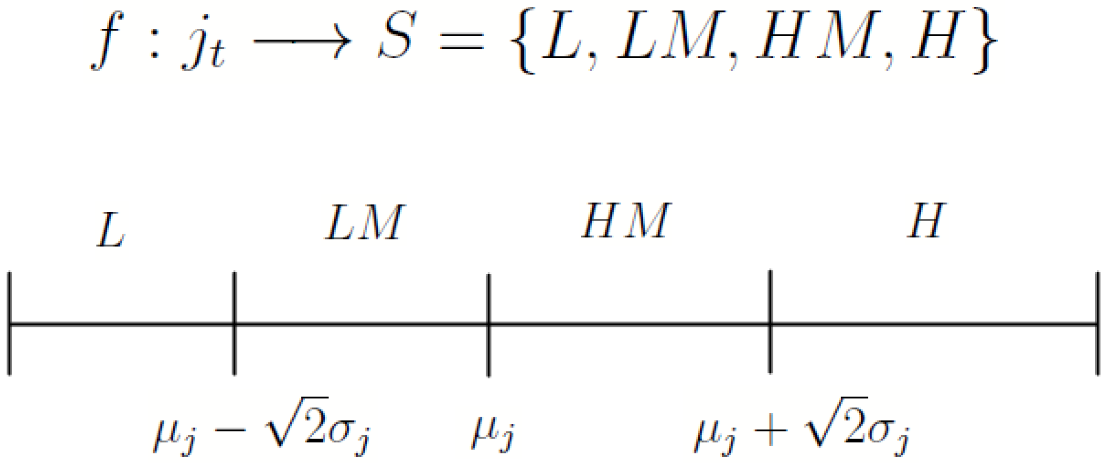
5.1. Mapping the Quantitative Financial Information to States

Consider a set of financial statements (i.e., a balance sheet, income statement, statement of cash flows and statement of retained earnings). These financial statements are each made up of a finite set of k variables, V = { 1 , 2 , , j , , k } , that are reported on each period. Without loss of generality, consider one of these variables, say j = e a r n i n g s . Finally, consider a representative individual. That is, consider an individual whose beliefs represent those of the market of interested users as a whole. I wish to apply I C ( M ) to determine the information content of the number that is reported for j each period to this representative user. Any discussion of information must begin with a state set; a set of states that the user feels that variable of interest j could possibly take on. In the context of the financial statements, j is continuous and does not admit a discrete state-probability distribution by itself. Rather, a function must be developed to map the variable of interest j to a discrete state-set (unless we are privy to the users’ true, perceived, continuous state-probability distribution for j; if we know this, then the uncertainty measure in Equation (3) can easily be modified to the continuous case). This immediately gives rise to the problem of which function to choose and how many states of the world does one consider that variable j could take on. Suppose I choose a function, f j t , which assigns each realization of j to one of four possible states where j t is the value of j reported for period t. The function I have in mind takes the following form:
f j t = H for j t > μ j t + 2 σ j t H M for μ j t j t μ j t + 2 σ j t L M for μ j t 2 σ j t j t < μ j t L for j t < μ j t 2 σ j t
where H, H M , L M and L represent that j t is in a high, high-medium, low-medium or low state, respectively. Notice that f j t is not defined for t = 1 . The idea is that I observe the reporting of j t and then map j t to one, and only one, state in my perceived state-space S = { H , H M , L M , L } based on the mean, μ j t , and standard deviation, σ j t , of the values of j that have been realized through time period t (I assume μ j and σ j both exist and are finite for t 2 ). Of course, this is not feasible initially for j 1 . Instead, I wait until j 2 is realized and then map j 1 to one of the four states in S using the function in Equation (3). The function f ( j t ) maps each earnings realization j t to one of four possible states in the state set S = { H , H M , L M , L } . Let the set X T = f j 1 , f j 2 , , f j T be the set of all values f ( j i ) , where T is the total number of realizations of j (for example, if five earnings realizations have occurred, a possible scenario could be X T = { H M , L M , L M , H , H M } ). Figure 4 illustrates f j t . At this point, one may feel that f ( j t ) , as specified in Equation (3), has been picked out of thin air and is rather arbitrary. Two sources of arbitrariness are perceived to be present. The first is: why choose four states? I admit that there is some arbitrariness in choosing four states. Mathematically, U ( P ) , and hence, I C M , depends on the number of states. Given equally probable states, the more states we add, the more uncertainty. Although the magnitude of I C M depends on the number of states, the interval and ratio properties of I C M do not. We will often want to compare the information contents of earnings releases within-firm across time and across firms. These comparisons do not depend on the number of states chosen, as long as we remain consistent in our choice. Finally, four states seem reasonably intuitive, as well. An individual may view a variable as being high, medium or low, but then wonder on which side of medium the variable is: closer to low or closer to high? Therefore, I model the individual as thinking of the continuous variable j as being in a high, high-medium, low-medium or low state.
The second source of arbitrariness lies in the specific choice of f ( j t ) . It turns out that the choice of f ( j t ) in Equation (3) is the only unbiased choice (unbiased in the sense that f ( j t ) is the only function depending on μ j t and σ j t that creates a mutually exclusive partition of S, which allows the possibility of assigning an equal proportion of j values to each half of the state set) of the function, given that the function depends on the mean and standard deviation of the variable j. Here, I appeal to Chebyshev’s theorem. Precisely stated, let c be any number greater than one. Then, for any sample of data, the proportion of observations lying fewer than c standard deviations from the sample mean is at least 1 1 c 2 . If c = 2 , then Chebyshev implies that at least 50 % of the observations of j lie within 2 standard deviations of μ (to see this, simply set 1 1 c 2 = 0 . 5 and solve for c). As defined in Equation (3), these values of j are mapped to two of the four states H M and L M , respectively. Thus, no more than 50 % of the values of j will be mapped to H and L. Note that Chebyshev does not say anything about the proportion of observations between μ and μ + c σ ; for example, the underlying distribution of j will determine this. The theorem only provides bounds (rather loose ones admittedly) on the proportion of observations that lie in the interval μ c σ , μ + c σ . Thus, Chebyshev directly implies the four-state mapping function as specified in Equation (3) if we want to partition the state-set S in such a way to make it possible for an equal proportion of j values to be mapped to each half of the state set. This ensures, as much as possible, that a particular value of j will not, mechanically, be more likely to be assigned to one of the states (As will be seen later, the function chosen in Equation (3) does not remove all determinism. There still remains the mechanical assigning of early observations of j to the states. This determinism, however, decreases rapidly over time, as will be seen with the example in Section 5.3.).

5.2. Forming the State-Probability Distributions P I and P A

With each value of j t now mapped to a particular state, I now can define the probability-state distributions, P I t and P A t , she or he perceives for j t at the beginning and end of period t, respectively, as follows (We will never be able to know the individuals’ true probability assignments, assuming they consciously form them. To apply an information theory approach, the best we can do is to proxy for these assignments in an intuitive way. f j t , P I and P A intend to do this.):
P I 1 = 1 4 , 1 4 , 1 4 , 1 4 = P I 2 = P A 1
P A t = P I t + 1 = a T , b T , c T , d T t 2
where:
  • a = count ( X T = L ) , b = count ( X T = L M )
  • c = count ( X T = H M ) , d = count ( X T = H )
Equation (4) reflects the assumption that, initially, she or he is completely uncertain as to which state j 1 will be in (intuitive with the notion that uncertainty is at its highest surrounding a firm’s first couple of earnings announcements due to the fact that we have little-to-no, prior, firm-specific history to utilize in forming an expectation), and therefore, she or he perceives the four states of S as being equiprobable. Upon receipt of the second message, j 2 (e.g., earnings in period two), she or he revises P I 2 accordingly to P A 2 . This probability distribution is also her or his initial probability distribution regarding the state that j 3 will be in and so forth. Thus, P A t = P I t + 1 for all t 2 . In forming P A t , I apply f ( j t ) to each of the prior realizations of j. This produces the set, X T = f j 1 , f j 2 , , f j T , T 2 , described in the previous section. I simply count the number of observations that were mapped to each state respectively and divide this frequency by the number of periods that have passed. This produces a frequency of occurrence for each state through time period T. I use this frequency to proxy for the ex ante probabilities that she or he forms for the states of S. An investor likely looks to past earnings in forming a state-probability distribution for future earnings. For example, suppose three out of the first five earnings announcements have been “high” relative to the mean. I model the user as thinking that the earnings in the sixth year will be “high” with 60% probability.

5.3. The Information Content, I C ( j ) , of Financial Statement Variable j

Following Equation (2), the information content, I C j t , of financial statement variable j at time t is as follows:
I C j t = | U j ( P I t ) U j ( P A t ) | U j ( P I t ) if U j ( P I t ) > U j ( P A t ) | U j ( P I t ) U j ( P A t ) | log ( 4 ) U j ( P I t ) if U j ( P I t ) < U j ( P A t ) 0 if U j ( P I t ) = U j ( P A t )
where P I t and P A t are as defined in Equations (4) and (5).
To illustrate, consider the annual earnings, j, of Apple Inc. from the date it went public through the present time (1981–2012) (earnings is the number reported annually for Compustat variable NI). Table 1 reports the results from applying Equations (3)–(6) to calculate I C j t for each of these thirty-three earnings realizations. The information content values, I C ( j t ) , are superscripted with “ ” if j t led to an uncertainty decrease or “ + ” if j t led to an uncertainty increase regarding future earnings realizations. To interpret I C j t from Table 1, observe the information content of earnings in 1981 ( 0 . 5 ). This means that the earnings “message” for 1981 decreased our uncertainty (our uncertainty regarding future realizations of earnings upon receiving the earnings “message” for 1981) by 50 % of the maximum by which it could have decreased it. One important point illustrated in Table 1 is that I C j 1 and I C j 2 are mechanical realizations. Since P I 1 = P A 1 by construction, the information content of first-period earnings will always be zero, independent of the company analyzed. Furthermore, the information content of second-period earnings will always be 0 . 5 independent of the company analyzed. This is due to the mathematical fact that, given any two real numbers a > b , the largest of the numbers a = μ + 2 2 σ and b = μ 2 2 σ , where μ and σ are the mean and standard deviation of the two numbers, respectively. This, along with Equations (3) and (5), immediately implies that the L M state and H M state will be assigned 1 2 probability. Once three earnings realizations have been realized, however, Equations (3) and (5) allow for a little more variation in uncertainty and, hence, variation in I C j t . As the number of earnings “messages” released by the company increases, I C j t becomes less and less mechanical. In essence, j t begins to determine I C j t rather than the mechanical construction set up in Equations (3) and (5). Thus, over time, I C j t better reflects the information content of j t (that is, as time increases, I C j t better reflects the intuitive definition of information offered in Section 4.1).
Keeping in mind Equations (3)–(6), Table 1 illustrates the idea that the earnings realizations, j t , or “messages” if you will, help us to update our priors. I C j t captures this updating and hence, the information contained in each earnings release. In essence, I C j t is a mathematical way to extract as much information as possible out of the earnings realizations. Of course, I C j t , as constructed, is only a function of the earnings realizations themselves and does not take into account any qualitative information surrounding an earnings release (such as contained in the footnotes or a press release, for example). Therefore, one could view I C j t as forming a lower bound on the information content of a given earnings release. I discuss this limitation in more detail later.
Appendix A illustrates how to use the measure developed in Equations (3)–(6) to assess the information content of the financial statements as a whole rather than one particular variable within those statements. This simply becomes an exercise in aggregation; however, one must pay attention to the fact that part of (if not all of) the information content of one variable may already be subsumed by another variable due to inter-variable dependencies within the financial statements.

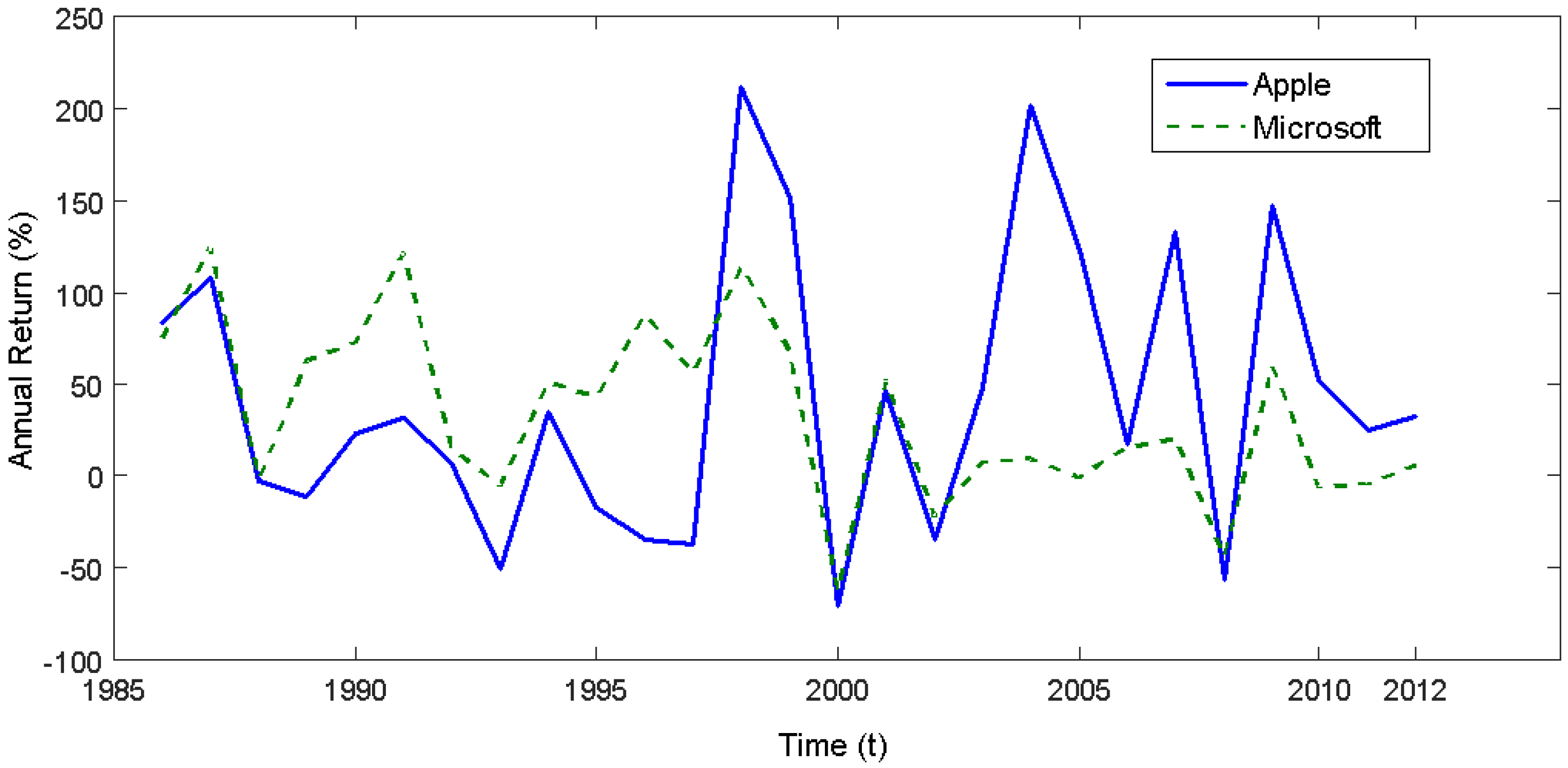
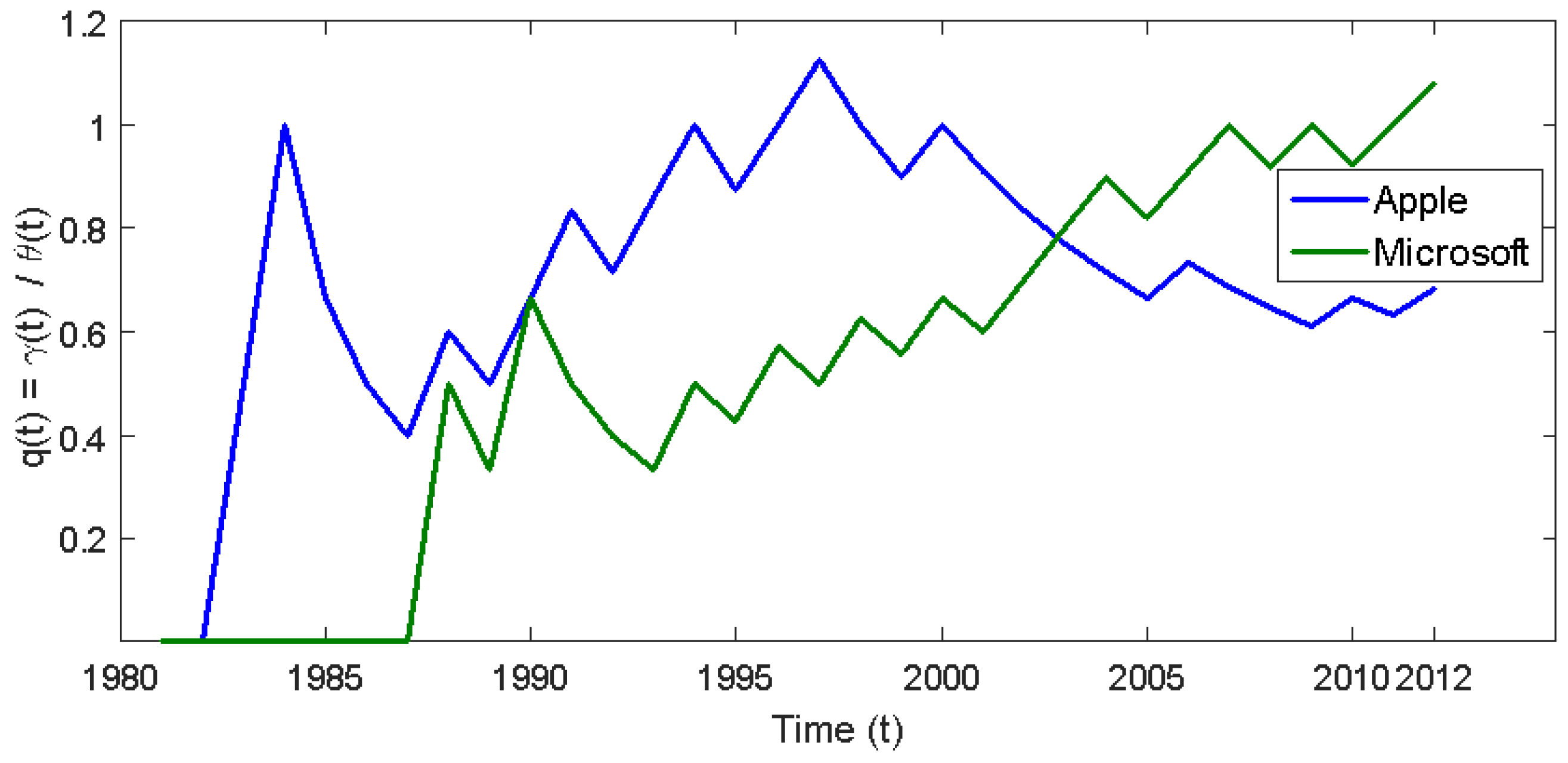
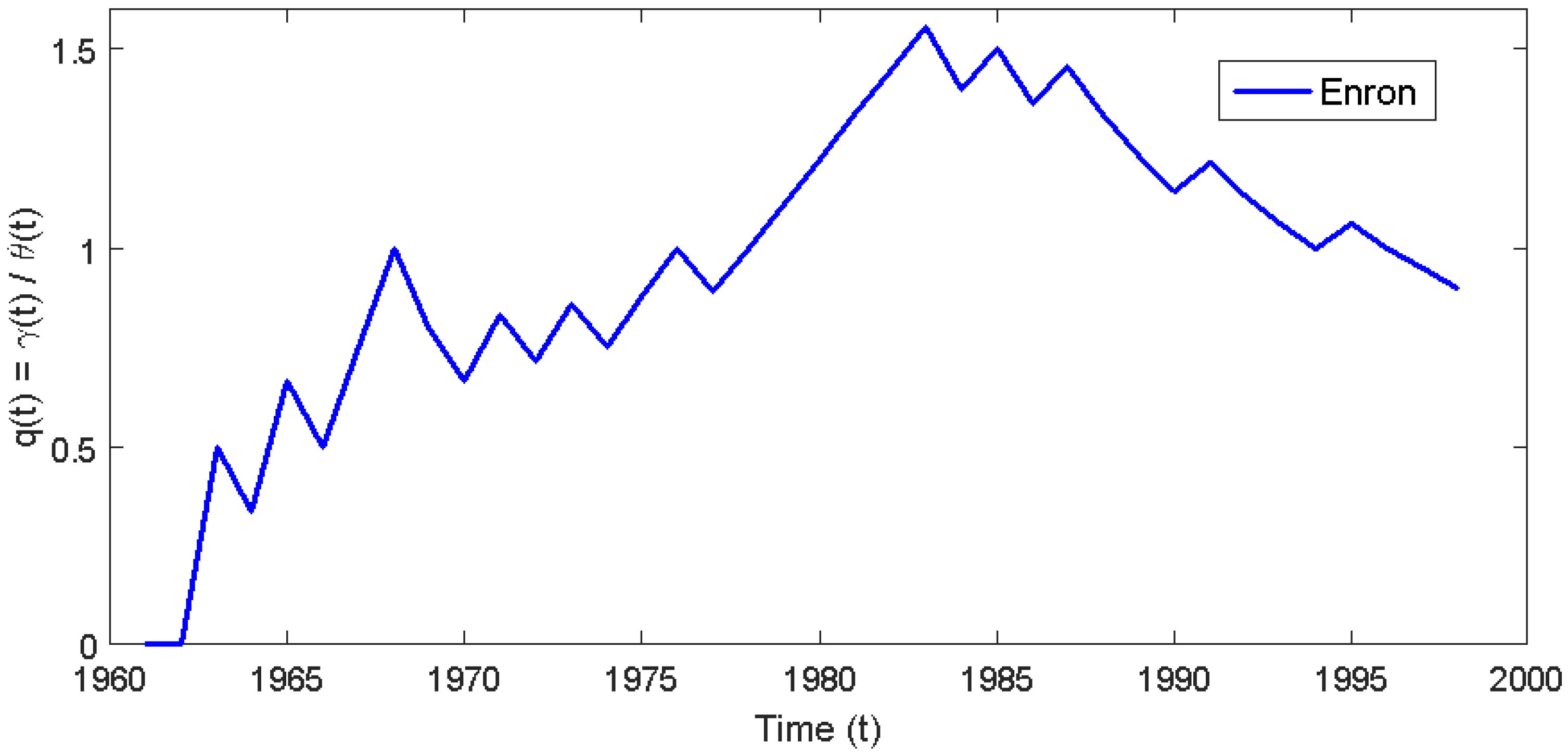
6. An Empirical Application

Theoretically, I C v j t is a perfectly valid measure of the information content of a given financial statement variable j at time period t. The question however becomes, does the framework adhered to in this paper hold in the real world? I acknowledge that it is unlikely that investors form state-probability distributions exactly the way specified in this paper. In fact, investors likely do not even consciously form state-probability distributions. Investors also likely do not consciously develop utility functions and seek to maximize them. Many economic studies, however, provide evidence consistent with the utility maximization assumption. The primary purpose of this paper is not to test the validity of the measures contained therein; I leave that to a future paper. That being said, there is one, interesting, potential application of I C v j t that I will offer (although there may be many applications once the measure is subjected to various empirical tests). You will notice from Table 1 that there have been 13 uncertainty-increasing annual earnings’ releases and 19 uncertainty-decreasing earnings’ releases over Apples’ thirty-three year history through 2012 (the average information content of the uncertainty-increasing releases is 0.1529, and the average information content of the uncertainty-decreasing releases is 0.0980). Ceteris paribus, this should be interpreted as a good thing, given one has a predisposition to favoring an uncertainty-decreasing information release over the opposite alternative. Over time, Apples’ earnings messages themselves are not neutral regarding uncertainty. That is, they tend to release earnings that decrease shareholders’ uncertainty regarding future earnings. Maybe insight could be obtained by examining the pattern of uncertainty-decreasing and uncertainty-increasing earnings’ releases over time within a firm and across firms. These patterns could provide insight into a given firms’ information environment relative to itself over time and relative to other companies. The patterns might also speak to the relative quality of earnings within a firm across time or across firms. I have the following idea in mind. Consider the function:
q ( t ) = γ ( t ) θ ( t )
where:
γ ( t ) = #  of uncertainty-increasing  earnings  realizations through time period  t θ ( t ) = #  of uncertainty-decreasing  earnings  realizations through time period  t
An interesting question is how this function behaves over time for a given firm and across firms. If we plot this function for Apple and Microsoft, the interesting picture in Figure 5 emerges. Analyzing Apple, we see that q ( t ) spikes initially and then fluctuates upwardly through year seventeen (1997) of their history. From year eighteen onward, q ( t ) follows a generally declining trend. As of now, the proportion of uncertainty-increasing earnings releases relative to uncertainty-decreasing ones is q A ( 2012 ) = 13 19 0 . 684 . Since 2000, q ( t ) < 1 for all t, and thus, Apple has been announcing fewer uncertainty-increasing earnings’ “messages”(see Table 1). Microsoft, on the other hand, has experienced a faster increase in q ( t ) as time has passed.
One interpretation of these observed patterns could be that Microsoft had a better information environment and higher quality earnings from 1985–2002 ceteris paribus. At some time t * between 2002 and 2003 (the time axis of Figure 5 is not depicted at a fine enough level of granularity to enable the user to easily see this), the two firms had identical proportions and q A ( t * ) = q M ( t * ) 0 . 8 . After this “critical” point, the information environment and earnings quality for Microsoft and Apple respectively have diverged. From the looks of the graph, I would have preferred Microsoft stock to Apple stock until sometime in 2002, when Apples’ stock looks more attractive. This prediction fits the risk-averse profile of the typical investor. Investors likely prefer companies with a better information environment (less information asymmetry). Thus, given a choice between a company announcing a higher (and generally increasing) ratio of uncertainty-increasing to uncertainty-decreasing earnings’ “messages” and a company whose same ratio is lower (and generally decreasing), they prefer the more transparent, less risky company. Based on the previous discussion and assuming q ( t ) adequately captures the strength of the information environment surrounding each company, Figure 5 implies that investors would prefer Microsoft over Apple from 1985–2002 and Apple over Microsoft from 2002–2012. Given earnings’ “messages” that increase uncertainty regarding future earnings, potential investors shy away from the Apple stock in the former time period in favor of the Microsoft stock. The risk-averse Apple shareholders would also react to the increased uncertainty and seek to sell their shares. They, however, would have difficulty finding a buyer due to reduced demand. Therefore, the price of Apple shares would fall, and the value of each shareholders’ investment would diminish. The opposite phenomenon would happen with the Microsoft shareholders during the early time period. These dynamics however would reverse after 2002.
Figure 6 plots the annual return from 1986–2012 for both Microsoft and Apple. Notice how the return of Microsoft is generally greater than Apple from 1986–2002, and then, consistent with the Figure 5 implications, the return drops below Apple and remains there (a graph of the annual closing share price for both companies reveals this even more clearly).
Figure 6 does not validate the measure of information content introduced in this paper. However, Figure 6 does offer some interesting insights into the potential usefulness of the measures introduced. The consistency of Figure 6 with the predictions implied from Figure 5 provides some evidence in favor of the measure (neither earnings, earnings per share nor return on assets tell the same story when graphed for both firms. There seems to be “hidden” information in earnings that I C v j t and, hence, q ( t ) capture).
As a simple test, I also regressed the annual returns of ten, large companies (over their respective lives to-date) on q with the following OLS, simple linear regression model:
R i t = α 0 + α 1 q i t + ϵ i t
where R i t is the annual return for firm i earned over time period t and q i t is the uncertainty ratio given in Equation (21) for firm i, respectively, as of the end of time period t (regressing returns on earnings, earnings per share, return on assets or their lagged values respectively for this sample does not produce a significant coefficient, and the average R 2 from these regressions is zero). Table 2 gives the companies used along with the number of observations for each company.
The coefficient on q i t was −0.9 (t-stat: 5 . 31 ), and the R 2 was 9.28% (I also regressed returns on lagged q i t to see how well the information measure can predict future returns. The coefficient was 0 . 39 (t-stat: 3 . 01 ), and the R 2 was 3 . 42 % . Furthermore, the correlation between earnings level and q i t was 0 . 06 .). This is consistent with the reasoning earlier. An increase in q from t to t + 1 implies that the t + 1 earnings announcement increased our uncertainty regarding future earnings for firm i. Risk-averse shareholders do not like increases in uncertainty and, thus, seek to sell their shares ceteris paribus. The reduced demand prevents the price from rising much (if at all), and therefore, returns fall. Interestingly, the explanatory power of Equation (8) for returns is 9.28%. One should notice at this point that the example given above (i.e., q ( t ) ) does not use, in any way, the magnitude of I C v j t . Instead, I simply counted the number of times the measure indicated an increase and decrease in uncertainty, respectively. A more direct attempt to validate I C v j t could be undertaken (I hope to test this idea and some others in a future paper) as follows. Suppose a set of analysts are forecasting earnings, E t + 1 , for period t + 1 for a given firm. These analysts observe earnings in period t and use this “message” to form their forecasts accordingly. It seems reasonable to assume that if E t increased their uncertainty regarding E t + 1 , then their subsequent forecasts will be more dispersed than if E t decreased their uncertainty regarding E t + 1 . This actually is assumed when analyst forecast dispersion is used as a proxy for uncertainty. One could test this assumption with I C v j t to see if, in fact, the assumption holds.

7. Broader Applications

Although the application chosen in this paper is a narrow (but important) financial accounting one, the measure introduced can be applied in a more general sense and is similar in thrust to [16]. The firm, or information consumer if you will, receives a vector of knowledge regarding the realization of any possible number of variables. Casting aside measurement issues for the moment (i.e., assuming the knowledge received by the information consumer is reliable and has been measured correctly), they only need a perceived state space for each variable in order to apply the measure and arrive at an estimate of the information content contained in the knowledge they received. Appendix A shows how this can be done if the vector consists only of knowledge regarding n financial statement variables. The theory applies to any vector of knowledge the information consumer receives, however, not just one particular type (e.g., financial knowledge). For example, the vector could provide knowledge regarding financial statement numbers (say current earnings and total assets) and the current level of information technology security within the firm. As long as these variables can be quantitatively summarized, the measure can use their realizations (along with past realizations) to estimate the change in uncertainty and, hence, information content of any particular realization using Equations (3)–(6).

8. Limitations

One limitation surrounding I C M as a measure of information content (I revert back to the original notation, without loss of generality, in the interest of simplicity. M is any message at a given point in time. P I is the individuals’ prior state-probability distribution, and P A is the individuals’ posterior state-probability distribution.) is the fact that I have defined I C ( M ) = 0 when U ( P I ) = U ( P A ) . To illustrate, consider the weather example from Section 4.1. Suppose initially P I = { rainy , sunny } = { 0 . 9 , 0 . 1 } . Next, the individual receives a weather forecast = M . Upon receiving and processing the knowledge contained in M, she or he updates her or his prior state-probabilities regarding the weather tomorrow to P A = { 0 . 1 , 0 . 9 } . It is trivial to check that U P I = U P A , and hence, as defined, I C M = 0 . Her or his overall level of uncertainty regarding which state will be realized has not changed upon receipt of M. She or he is more certain, after M, that it will rain tomorrow than she or he was before M. However she or he is less certain that it will be sunny tomorrow. The increase in certainty regarding the rainy state is exactly offset by the decrease in certainty regarding the sunny state. Thus, quantitatively, her or his overall uncertainty remains the same. Qualitatively though, one would argue that M does contain information. M informs her or him that she or he should probably bring an umbrella to the beach and leave her or his sunscreen at home! The limitation highlighted above is that I C ( M ) captures only the quantitative information content of M ([17] points out that the Shannon entropy function is a measure of uncertainty, “but it is uncertainty when all the information we have consists of just these numbers ”). There often will be qualitative information contained in M. In this case, I C ( M ) does not capture this. This limitation is particularly important in an accounting context if we use I C ( M ) to measure the information content of the financial statements. I have been careful to say that I C ( M ) captures the information content of the quantitative portions of the financial statements. Other “messages” within the financial statements are the footnotes. It is interesting to think about the problem of quantifying the information content of the qualitative footnotes. Recent advances in textual analysis, including readability measures and positive/negative tone measures for example, have helped researchers deal with this problem. One could think of I C ( M ) as forming a lower bound on the information content of the financial statements. Combining I C ( M ) with some of these other measures of footnote information content would provide a more robust measure.
Another limitation lies in the reliability of the accounting numbers themselves. Since the measure is a function of accounting variables, which are subjective estimates of the firm, it is subject to at least as much underlying noise already contained in the underlying variables. Earnings, for example, is an accrual number that captures cash flows in expectation. To the extent companies engage in earnings management, the measure noisily captures the true information. For example, I applied the measure to Enron’s earnings numbers over 1962–2000 (The Northern Natural Gas company was formed in 1932 and later reorganized into a holding company and renamed InterNorth. Enron was organized as the main subsidiary of InterNorth in 1979. I used data on Northern Natural Gas going back as far as Compustat allows (1962).). Figure 7 plots the information content ratio, q ( t ) , from Equation (7) and was highest in 1984, the year prior to Kenneth Lay being hired as CEO. From then on, the ratio of uncertainty increasing earnings announcements relative to uncertainty decreasing earnings announcements declined. Thus, over the 16-year period from 1985–2000, the measure suggests that Enron’s earnings contained less and less uncertainty regarding the state of future earnings, yet we know (ex post) that Enron filed for bankruptcy in 2001.

9. Conclusions

This paper defines information as that subset of knowledge that changes a users’ uncertainty regarding the state a particular variable of interest will assume in the future. This definition is firmly grounded in an information theory framework. From this definition, I then develop a measure of the information content of a message in general. Shannon entropy, as a measure of uncertainty, is applied to form this measure. Several examples, along the way, illustrate how the measure can be applied.
I also argue that accounting fits within a classical communication system framework. I apply the measure developed to the problem of measuring the information content of “messages” that are transmitted from the accounting and reporting process to interested users. The messages are of interest to users because they contain information regarding future variables of interest (e.g., earnings, cash flows, etc.). I modify the general measure to form a specific measure of the information content of accounting “messages” (e.g., earnings, assets, financial statements). I then provide a firm-specific example where the “message” is period t earnings and the variable of interest is period t + 1 earnings. This example provides some evidence validating the measures’ construct validity.
When applied to an accounting context, the underlying idea is that the quantitative financial statements, in aggregate and at the variable level, contain information that, at first glance, cannot be observed from the numbers themselves. The measure I C v j t , however, is able to extract this information in a way that is both interesting and insightful.

10. Future Research

This paper only scratches the surface regarding how information theory can be applied to an accounting context. If one accepts the particular way in which I apply information theory, then there are a host of questions surrounding the measures introduced. For example, can the measures predict bankruptcies, earnings restatements or other firm-level calamities? Are the measures consistent with the more traditional earnings-response coefficient information content measure? Do the measures proxy for firm-level risk (both creditor and shareholder risk; evidence of a higher cost of capital for those firms with lower information content financial statements, ceteris paribus, may provide evidence that the measures can capture risk)?
The measures introduced may also provide an avenue by which to approach deeper, more fundamental questions. For example, what is the optimal reporting period from an investors’ standpoint for a given firm or across firms? In fact, applying the measures introduced to Apple and Microsoft quarterly earnings instead of annual earnings provides earlier evidence that Apple would have been a better investment than Microsoft. This is consistent with the notion that investors would want both companies to report quarterly instead of annually if they had to choose between the two. Of course, Microsoft would choose annually over quarterly reporting given the same choice ceteris paribus. This is consistent with a favorable view of the Securities and Exchange Commission fulfilling its duty of protecting investors.
Another fundamental question the measure could render attainable is at what level of aggregation should the financial statements be presented? If all of the information contained in a particular variable j is already subsumed by some combination of the other variables, then maybe j should not be reported within the statements. The costs of processing the redundant information in j outweigh the benefits.
These questions, particularly the more theoretical ones, are fundamental to understanding accounting as a communication system. Hopefully, this paper has made the prospect of providing answers to these questions seem a little more attainable.
multiple

Acknowledgments

I gratefully acknowledge the helpful comments and suggestions of Roger Debreceny and John Fellingham, as well as workshop participants at Binghamton University and at the University of Kentucky.

Conflicts of Interest
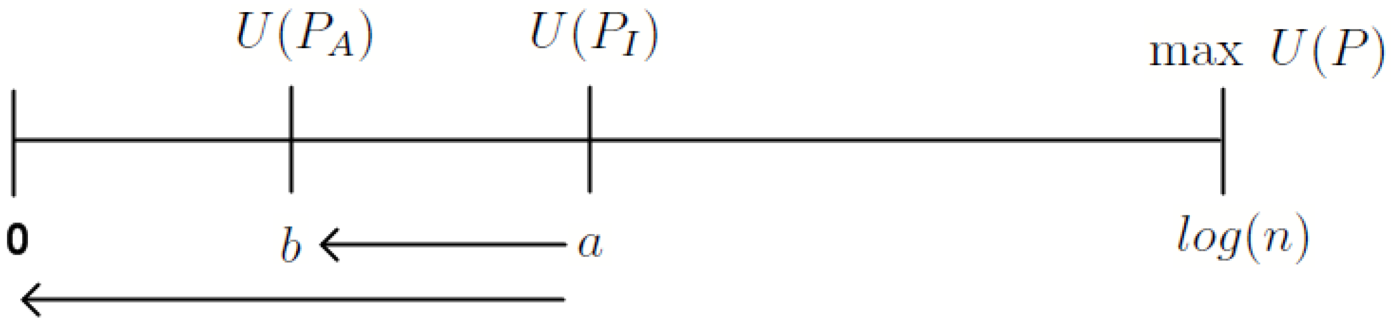
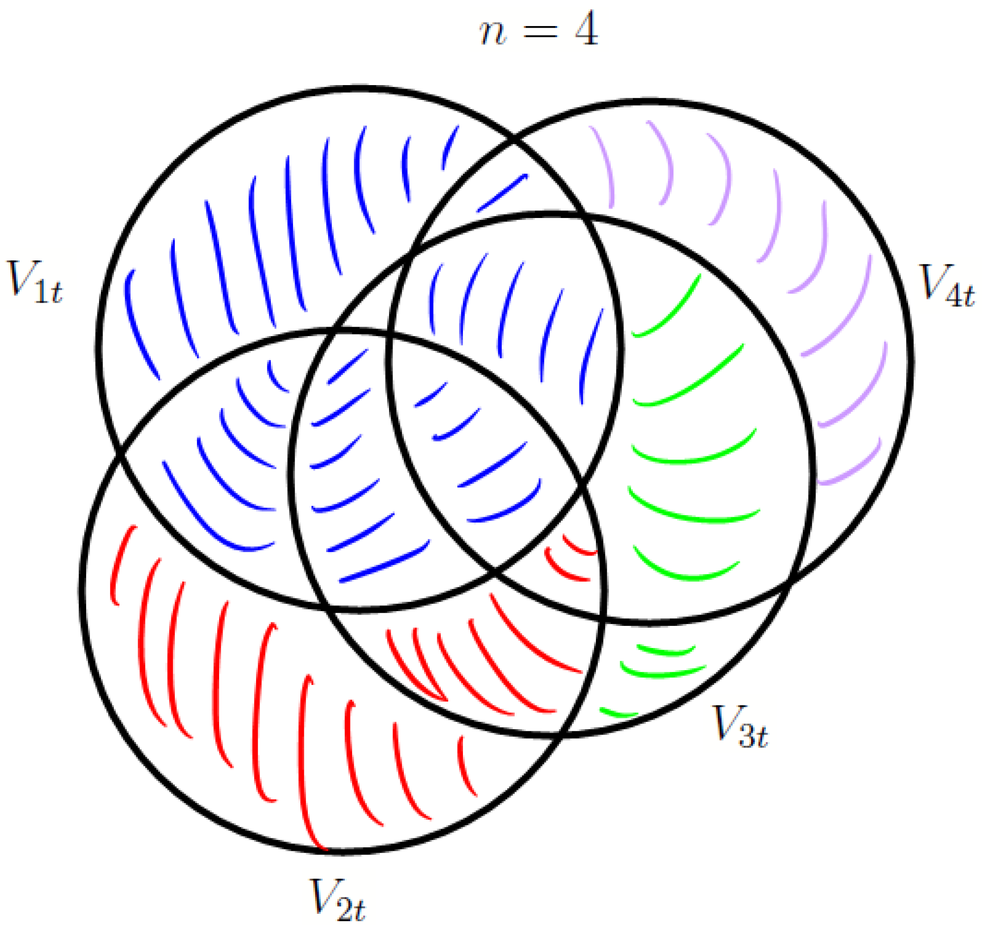
The author declares no conflict of interest.

Appendix A. The Information Content, I C F , of the Financial Statements

Up to this point, I have focused on the information content, I C j t , of variable j in time period t. Suppose a set of financial statements, F t , is released at time period t. Let this set be described as follows (I change notation here, by allowing v j t to represent “variable j t ”. Note also that n now refers to the number of variables instead of the number of states. The number of states is fixed, by assumption, at four, while the number of variables in the financial statements is n.):
F t = { v 1 t , v 2 t , , v n t }
That is, at time period t, we have a set of financial statements comprised of n variables. Now, I wish to assess I C F t . Simply calculating the sum j = 1 n I C v j t does not quite work, however, since some of the information in any one of the n variables will already be contained in one, or more, of the other variables. Summing in this way will lead to double counting this information.
Figure 7 illustrates what I would like to do when n = 4 , for example. The shaded regions in Figure A1 begin by shading in the information provided by v 1 t with blue. Next, I move counterclockwise and shade in (red) the portion of v 2 t not shaded blue. I then shade in (green) the portion of v 3 t not already shaded blue or red. Finally, I shade in (purple) the portion of v 4 t not already shaded blue, red or green. The information content of the financial statements is then equal to the sum of the information contents of each of the colored regions. This process of “sweeping” out the information contents of each financial statement variable one at a time (without double counting) can be accomplished by using the principle of inclusion-exclusion from mathematical set theory. Equation (A1) captures the idea for n = 3 :
I C F t = j = 1 3 I C v j t I C v 1 t I C v 2 t I C v 1 t I C v 3 t I C v 2 t I C v 3 t + I C v 1 t I C v 2 t I C v 3 t
As given in Equation (A1), F t is a set consisting of n variables. We can measure the size of the information contained in F t by considering the size of the information (information contents) contained in each of these variables. The problem is, when summing over these sets, we over-estimate by counting intersections more than once. Equation (A2) excludes these “over-included” intersections. In the process, we exclude too much and, thus, need to add back a final term (one can readily check, with a Venn diagram, that the above formula is correct). The formula above is a special case of the general formula, attributed to Abraham De Moivre, an 18th century French mathematician. The general formula for evaluating the size of a given set by considering the sizes of the different, non-mutually exclusive subsets of which it is comprised is given in Equation (A3). I express the formula in the context of the present discussion, and therefore, information content ( I C ) is the “size of the information”.
I C F t = i = 1 n I C v i t i , j : 1 i < j n I C v i t I C v j t + i , j , k : 1 i < j < k n I C v i t I C v j t I C v k t + ( 1 ) n 1 I C v 1 t I C v n t
I admit that Equation (A3) is cumbersome to follow. It is the classic example of condensing something rather complicated into one precise formula. Nevertheless, one can check their understanding at this point by plugging n = 3 into Equation (A3); you should recover Equation (A2). Notice the alternating signs. This helps to ensure that anything we over-include in summing over the information contents of all of the variables we make sure to exclude. Applying Equation (A3), when n = 4 , will precisely give the intuitive result in Figure A1.
What is the point of all of the math you ask? The idea is that aggregating is a delicate task that requires caution. We need to ensure that we only “sweep” out information content once, as in Figure A1. Furthermore, Equation (A3) highlights the importance of defining the intersections. I turn next to this problem.
I will define the intersection of information content as follows:
I C v i t I C v j t = 1 ξ 2 I C v k * t i = I * n 1 j = i + 1 n ρ i j t
where:
  • v k * t = the variable with the smallest information content, i k * j
  • I * = the starting variable index
  • n = the ending variable index
  • ρ i j t = the Pearson correlation between i and j through time t 2
  • ξ = the # of variables intersected
Figure A1. Information content of four-variable financial statements. This figure illustrates the non-overlapping information content of the financial statements reporting on four variables only.
Information 07 00048 g008
Equation (A4) is a general expression for the intersection of information contents between any combination of variables beginning with variable i through variable j. Equation (A4) calculates the information content of variable i that is already subsumed in the other variables up through variable j. Everything needed in Equation (A3) to calculate I C F t , given the financial statement variables, is provided by Equation (A4). Precisely, given variables v i t , , v j t , Equation (A4) is the average of all possible pair-wise Pearson correlations multiplied by the smallest information content. This is consistent with the notion that the information content of the intersection can be no greater than the smallest information content. For example, suppose you are given I C v 1 t = 0 . 2 , I C v 2 t = 0 . 3 , I C v 3 t = 0 . 1 and ρ 12 = 0 . 6 , ρ 13 = 0 . 9 and ρ 23 = 0 . 95 . The information content common to all three variables is 0 . 1 * 1 3 2 * ( 0 . 6 + 0 . 9 + 0 . 95 ) 0 . 08167 . Although this is likely an estimate, it is intuitive with the notion that the information content common to all three variables is an increasing function of the correlation between the variables. The absolute value sign prevents the meaningless case of negative joint information. Although any two variables could be negatively correlated, knowing this is just as informative as knowing that they are positively correlated with each other! In other words, I do not lose anything by disregarding the sign of the correlation between the two variables.
One will recall from the Apple Inc. example that I C v j t can be signed (superscripted) to indicate whether uncertainty increased or decreased. When aggregating the information contents, however, I disregard whether v j t increases or decreases the individuals’ uncertainty. I assume that a realization of v j t , which increases our uncertainty regarding future realizations of v j , is equally as informative as a realization of v j t , which decreases our uncertainty regarding future realizations of v j . Therefore, theoretically, 0 I C F t n (recall that 0 I C v j t 1 for all j). Calculating I C F t = 4 , for example, where F t consists of ten variables, implies that the information content of F t is 40 % of the maximum amount it could have theoretically been (60% shy of “perfect” information; perfect in the sense that all of the information contained in each variable j is unique to j and is equal to one;I call this percentage I C * * F t in Appendix B). A different way to express the information content of the financial statements, which may be more meaningful, is to divide I C F t by the sum of the individual variable information contents. If there is no information common to any of the variables, then I C F t would equal this sum, and we could say that the financial statements contained maximum information relative to the information contents of each of the variables therein. Thus, a more meaningful measure of financial statement information content is given below:
I C * F t = I C F t i = 1 n I C v i t
The above discussion implies that I C F t is maximized, theoretically, when each of the financial statement variables is independent of the others. If this is the case, the numerator and denominator of Equation (A5) are equal, and I C * F t = 1 . The equivalent of this pictorially is where the circles in Figure A1 do not intersect each other. The converse of this occurs when each of the n variables is perfectly correlated with each of the others. If this is the case, I C F t = I C v k * t and I C * F t = I C v k * t / i = 1 n I C v i t . Pictorially, this implies that the circles in Figure A1 are perfectly superimposed over each other, such that the information in the smallest information content variable is the most the user can obtain from the statements.
Next, I provide an empirical example to help illustrate some of the potential applications of I C v j t . In Appendix B, I continue with the Apple Inc. example to illustrate I C * F t and I C * * F t (in Appendix B, I deal with the problem of signing I C F t ; see Equations (B1) and (B2)).

Appendix B. The Information Content of Apple’s Financial Statements

To illustrate the calculation of I C F t for a given company, consider Apple Inc. over the time period 1980–1990. Without loss of generality, suppose Apple’s financial statements, for each of these years, consisted of only four variables: earnings, total revenue, total assets and total liabilities (variables N I , R E V T , T A and T L , respectively, from Compustat). Thus, we consider the following set:
F t = e a r n i n g s t , t o t a l r e v e n u e t , a s s e t s t , l i a b i l i t i e s t = v 1 t , v 2 t , v 3 t , v 4 t
First, calculate the correlations ρ i j t between each pair of variables through each time period t 2 . Thus, for each time period, a vector of six correlations is produced. For example, through t = 5 , the correlation between earnings and total revenue is ρ 12 5 = 0 . 7726 . These correlations are listed in Table B1.
Table B1. Correlations among Apple’s financial statement variables. This table reports the correlations of Apple’s financial statement variables (earnings, total revenue, total assets and total liabilities) in the Appendix B example.
Yeart | ρ 12 t | | ρ 13 t | | ρ 14 t | | ρ 23 t | | ρ 24 t | | ρ 34 t |
198121.00001.00001.00001.00001.00001.0000
198230.99440.99490.99750.97860.98450.9995
198340.96320.98340.93580.98910.99220.9822
198450.77260.82500.66540.99330.98670.9702
198560.66880.73320.59730.99420.99320.9823
198670.72220.83350.78040.98250.98270.9895
198780.84470.90240.89110.98960.98800.9931
198890.92960.93760.96120.99410.99170.9885
1989100.96230.96650.97860.99700.99430.9928
1990110.97370.97620.98100.99780.99350.9940
Next, calculate the information contents of each of the four variables over the 1980–1990 time frame. These are displayed in Table B2. Now, apply Equations (B1) and (B2) to calculate the information content of the financial statements. For example, to illustrate I C F 8 , you get the following:
I C F 8 = I C v 18 + I C v 28 + I C v 38 + I C v 48 I C v 18 I C v 28 I C v 18 I C v 38 I C v 18 I C v 48 I C v 28 I C v 38 I C v 28 I C v 48 I C v 38 I C v 48 + I C v 18 I C v 28 I C v 38 + I C v 18 I C v 28 I C v 48 + I C v 18 I C v 38 I C v 48 + I C v 28 I C v 38 I C v 48 I C v 18 I C v 28 I C v 38 I C v 48 = 0 . 0762 + 0 . 4142 + 0 . 0432 + 0 . 0432 ( 0 . 0762 * 0 . 8447 ) ( 0 . 0432 * 0 . 9024 ) ( 0 . 0432 * 0 . 8911 ) ( 0 . 0432 * 0 . 9896 ) ( 0 . 0432 * 0 . 9880 ) ( 0 . 0432 * 0 . 9931 ) 0 . 0432 3 * ( 0 . 8447 + 0 . 9024 + 0 . 9896 ) 0 . 0432 3 * ( 0 . 8447 + 0 . 8911 + 0 . 9880 ) 0 . 0432 3 * ( 0 . 9024 + 0 . 8911 + 0 . 9931 ) 0 . 0432 6 * ( 0 . 8447 + 0 . 9024 + 0 . 8911 + 0 . 9896 + 0 . 9880 + 0 . 9931 ) 0 . 4278
Now, use Equation (A5) to express I C F 8 in percentage terms and derive I C * F 8 :
I C * F 8 = 0 . 4278 ( 0 . 0762 + 0 . 4142 + 0 . 0432 + 0 . 0432 ) 0 . 7417 or 74 %
Thus, the information content of Apples’ 1987 financial statements was 74 % of the maximum it could have been, given the information contained in the variables of which the statements were comprised. That is, given the information contents of each of the variables, if the variables were all independent, the maximum information content would have been i = 1 4 I C v i t = 0 . 5768 . However, given the additional constraint that the variables not only be independent, but also have maximal information themselves (i.e., I C v i t = 1 for all i), the information content of the 1987 financial statements was I C * * F t = I C F t / n = 0 . 4278 / 4 0 . 1070 . Thus, the 1987 statements changed our uncertainty regarding future financial statements 10 . 7 % of the maximum amount it possibly could have. Note in Table B2 that this was an uncertainty-increasing change. Notice that I have not signed I C F t . To accomplish this, consider the proportion of variables that increased uncertainty to those that decreased uncertainty. Call this function p ( t ) :
p ( t ) = ϕ ( t ) ψ ( t )
where:
ϕ ( t ) = the #  of uncertainty-increasing  variables  at time  t ψ ( t ) = the #  of uncertainty-decreasing  variables  at time  t
Table B2. Information content of Apple’s financial statement variables. This table reports the information content of Apple’s financial statement variables (earnings, total revenue, total assets and total liabilities) in the Appendix B example using Equation (B2).
Yeart IC v 1 t IC v 2 t IC v 3 t IC v 4 t
198010.0000000
198120.5000 0.5000 0.5000 0.5000
198230.0817 0.0817 0.0817 0.0817
198340.0755 + 0.0755 + 0.0755 + 0.0755 +
198450.3709 + 0.3709 + 0.0290 0.3709 +
198560.0870 0.1402 + 0.0282 + 0.0870
198670.0821 0.3247 0.3787 + 0.1699 +
198780.0762 0.4142 + 0.0432 + 0.0432 +
198890.1737 + 0.0384 0.0384 0.0384
1989100.0552 0.1441 0.0415 0.0297 +
1990110.1808 + 0.1808 + 0.0196 + 0.0950
Thus, the information content of the financial statements at time t can be signed as follows:
I C F t = I C F t + if p ( t ) > 1 I C F t if p ( t ) < 1
Now, if p ( t ) = 1 , then half of the variables increased our uncertainty regarding future realizations of those variables, and half of the variables decreased our uncertainty. In this case, we consider the magnitude of the information contents of the uncertainty-increasing and uncertainty-decreasing variables. Define a new function as follows:
z ( t ) = ω ( t ) ζ ( t )
where:
ω ( t ) = the mean information content of uncertainty-increasingvariables at time t ζ ( t ) = the mean information content of uncertainty-decreasingvariables at time t
The information content of the financial statements in this case is defined as follows:
I C F t = I C F t + if z ( t ) > 0 I C F t if z ( t ) 0 if p ( t ) = 1
Table B3 reports I C F t , I C * F t and I C * * F t for Apple from 1980–1990.
Table B3. Information content of Apple’s financial statements (1980–1990). This table reports the information content of Apple’s financial statements using each the measures from Equations (A5) and (B2), respectively.
Yeart IC F t IC * F t IC * * F t
19801000
198120.5000 0.2500 0.1250
198230.0837 0.2563 0.0209
198340.0813 + 0.2692 + 0.0203 +
198450.5135 + 0.4497 + 0.1283 +
198560.1837 0.5367 0.0459
198670.4132 + 0.4324 + 0.1033 +
198780.4278 + 0.7416 + 0.1069 +
198890.1775 0.6144 0.0443
1989100.1469 0.5425 0.0367
1990110.1865 + 0.3916 + 0.0466 +

References

  1. Shannon, C. A mathematical theory of communication. Bell Syst. Tech. J. 1948, 27, 379–423. [Google Scholar] [CrossRef]
  2. Beaver, W.H. The information content of annual earnings announcements. J. Account. Res. 1968, 6, 67–92. [Google Scholar] [CrossRef]
  3. Bowen, R.M.; Burgstahler, D.; Daley, L.A. The incremental information content of accrual versus cash flows. Account. Rev. 1987, 62, 723–747. [Google Scholar]
  4. Freeman, R.N.; Tse, S. The multiperiod information content of accounting earnings: Confirmations and contradictions of previous earnings reports. J. Account. Res. 1989, 27, 49–79. [Google Scholar] [CrossRef]
  5. Landsman, W.R.; Maydew, E.L. Has the information content of quarterly earnings announcements declined in the past three decades? J. Account. Res. 2002, 40, 797–808. [Google Scholar] [CrossRef]
  6. Waymire, G. Additional evidence on the information content of management earnings forecasts. J. Account. Res. 1984, 22, 703–718. [Google Scholar] [CrossRef]
  7. Beaver, W.; Lambert, R.; Morse, D. The information content of security prices. J. Account. Econ. 1980, 2, 3–28. [Google Scholar] [CrossRef]
  8. Bedford, N.M.; Baladouni, V. A communication theory approach to accountancy. Account. Rev. 1962, 37, 650–659. [Google Scholar]
  9. Theil, H. Economics and Information Theory; North Holland Publishing Co.: Amsterdam, The Netherlands, 1967; Volume 7. [Google Scholar]
  10. Theil, H. On the use of information theory concepts in the analysis of financial statements. Manag. Sci. 1969, 15, 459–480. [Google Scholar] [CrossRef]
  11. Gibbs, J.W. On the equilibrium of heterogeneous substances. Am. J. Sci. 1878, 96, 441–458. [Google Scholar] [CrossRef]
  12. Lev, B. The aggregation problem in financial statements: An informational approach. J. Account. Res. 1968, 6, 247–261. [Google Scholar] [CrossRef]
  13. Lev, B. The informational approach to aggregation in financial statements: Extensions. J. Account. Res. 1970, 8, 78–94. [Google Scholar] [CrossRef]
  14. Cover, T.M.; Thomas, J.A. Elements of Information Theory, 2nd ed.; John Wiley & Sons: Hoboken, NJ, USA, 2006. [Google Scholar]
  15. Christensen, J.A.; Demski, J. Accounting Theory; Irwin/McGraw-Hill: New York, NY, USA, 2002. [Google Scholar]
  16. Sun, L.; Srivastava, R.P.; Mock, T.J. An information systems security risk assessment model under the dempster-shafer theory of belief functions. J. Manag. Inf. Syst. 2006, 22, 109–142. [Google Scholar] [CrossRef]
  17. Jaynes, E.T. Probability Theory: The Logic of Science; Cambridge University Press: Cambridge, UK, 2003. [Google Scholar]
Figure 1. Accounting as a communication system. This figure displays how accounting fits into the classical framework of a communication system.
Information 07 00048 g001
Figure 2. Uncertainty increasing message. This figure illustrates how uncertainty increases relative to the maximum amount by which it could have increased.
Information 07 00048 g002
Figure 3. Uncertainty decreasing message. This figure illustrates how uncertainty decreases relative to the maximum amount by which it could have decreased.
Information 07 00048 g003
Figure 4. Earnings state mapping function. This figure depicts the earnings state mapping function, f ( j t ) from Equation (3).
Information 07 00048 g004
Figure 5. Uncertainty ratio for Apple and Microsoft. This figure plots the earnings uncertainty ratio in Equation (7) for Apple and Microsoft from their inceptions as companies through 2012.
Information 07 00048 g005
Figure 6. Annual return for Apple and Microsoft. This figure plots the annual share price return for Apple and Microsoft from their inceptions as companies through 2012.
Information 07 00048 g006
Figure 7. Uncertainty ratio for Enron (1962–2012). This figure plots the earnings uncertainty ratio in Equation (7) for Enron over the period 1962–2000. The Northern Natural Gas company was formed in 1932 and later reorganized into a holding company and renamed InterNorth. Enron was organized as the main subsidiary of InterNorth in 1979. I used earnings data on Northern Natural Gas going back as far as Compustat allows (1962).
Information 07 00048 g007
Table 1. Information content of Apple Inc. earnings (1980–2012). This table reports the information content of each of Apple’s thirty-three earnings releases from its inception as a company through 2012 using the information content measure from Equation (A1).
t j t ($millions) P It P At IC ( j t )
1980$11.70 1 / 4 , 1 / 4 , 1 / 4 / 1 / 4 1 / 4 , 1 / 4 , 1 / 4 / 1 / 4 0
1981$39.42 1 / 4 , 1 / 4 , 1 / 4 / 1 / 4 0 , 1 / 2 , 1 / 2 , 0 0 . 5
1982$61.306 0 , 1 / 2 , 1 / 2 , 0 0 , 1 / 3 , 2 / 3 , 0 0 . 0817
1983$76.714 0 , 1 / 3 , 2 / 3 , 0 0 , 1 / 2 , 1 / 2 , 0 0 . 0755 +
1984$64.055 0 , 1 / 2 , 1 / 2 , 0 1 / 5 , 1 / 5 , 3 / 5 , 0 0 . 3710 +
1985$61.223 1 / 5 , 1 / 5 , 3 / 5 , 0 1 / 6 , 1 / 6 , 2 / 3 , 0 0 . 0870
1986$153.963 1 / 6 , 1 / 6 , 2 / 3 , 0 0 , 5 / 7 , 1 / 7 , 1 / 7 0 . 0821
1987$217.496 0 , 5 / 7 , 1 / 7 , 1 / 7 0 , 3 / 4 , 1 / 8 , 1 / 8 0 . 0762
1988$400.258 0 , 3 / 4 , 1 / 8 , 1 / 8 0 , 2 / 3 , 2 / 9 , 1 / 9 0 . 1738 +
1989$454.033 0 , 2 / 3 , 2 / 9 , 1 / 9 0 , 7 / 10 , 1 / 10 , 1 / 5 0 . 0552
1990$474.895 0 , 7 / 10 , 1 / 10 , 1 / 5 0 , 7 / 11 , 2 / 11 , 2 / 11 0 . 1809 +
1991$309.841 0 , 7 / 11 , 2 / 11 , 2 / 11 0 , 7 / 12 , 1 / 4 , 1 / 6 0 . 1088 +
1992$530.373 0 , 7 / 12 , 1 / 4 , 1 / 6 0 , 8 / 13 , 4 / 13 , 1 / 13 0 . 1051
1993$86.589 0 , 8 / 13 , 4 / 13 , 1 / 13 0 , 4 / 7 , 2 / 7 , 1 / 7 0 . 1838 +
1994$310.178 0 , 4 / 7 , 2 / 7 , 1 / 7 0 , 8 / 15 , 1 / 3 , 2 / 15 0 . 0335 +
1995$424 0 , 8 / 15 , 1 / 3 , 2 / 15 0 , 9 / 16 , 3 / 8 , 1 / 16 0 . 1086
1996$(816) 0 , 9 / 16 , 3 / 8 , 1 / 16 1 / 17 , 8 / 17 , 8 / 17 , 0 0 . 0218 +
1997$(1045) 1 / 17 , 8 / 17 , 8 / 17 , 0 1 / 9 , 7 / 18 , 1 / 2 , 0 0 . 1605 +
1998$309 1 / 9 , 7 / 18 , 1 / 2 , 0 2 / 19 , 7 / 19 , 10 / 19 , 0 0 . 0160
1999$601 2 / 19 , 7 / 19 , 10 / 19 , 0 1 / 10 , 7 / 20 , 11 / 20 , 0 0 . 0172
2000$786 1 / 10 , 7 / 20 , 11 / 20 , 0 2 / 21 , 8 / 21 , 10 / 21 , 1 / 21 0 . 3553 +
2001$(25) 2 / 21 , 8 / 21 , 10 / 21 , 1 / 21 1 / 11 , 9 / 22 , 5 / 11 , 1 / 22 0 . 0067
2002$65 1 / 11 , 9 / 22 , 5 / 11 , 1 / 22 2 / 23 , 10 / 23 , 10 / 23 , 1 / 23 0 . 0088
2003$69 2 / 23 , 10 / 23 , 10 / 23 , 1 / 23 1 / 12 , 5 / 12 , 11 / 24 , 1 / 24 0 . 0104
2004$276 1 / 12 , 5 / 12 , 11 / 24 , 1 / 24 2 / 25 , 11 / 25 , 11 / 25 , 1 / 25 0 . 0081
2005$1335 2 / 25 , 11 / 25 , 11 / 25 , 1 / 25 1 / 13 , 11 / 26 , 6 / 13 , 1 / 26 0 . 0094
2006$1989 1 / 13 , 11 / 26 , 6 / 13 , 1 / 26 2 / 27 , 4 / 9 , 11 / 27 , 2 / 27 0 . 1995 +
2007$3496 2 / 27 , 4 / 9 , 11 / 27 , 2 / 27 1 / 14 , 4 / 7 , 2 / 7 , 1 / 14 0 . 0514
2008$4834 1 / 14 , 4 / 7 , 2 / 7 , 1 / 14 0 , 23 / 29 , 4 / 29 , 2 / 29 0 . 3918
2009$8235 0 , 23 / 29 , 4 / 29 , 2 / 29 0 , 5 / 6 , 1 / 15 , 1 / 10 0 . 1228
2010$14,013 0 , 5 / 6 , 1 / 15 , 1 / 10 0 , 25 / 31 , 4 / 31 , 2 / 31 0 . 0629 +
2011$25,922 0 , 25 / 31 , 4 / 31 , 2 / 31 0 , 27 / 32 , 3 / 32 , 1 / 16 0 . 1236
2012$41,733 0 , 27 / 32 , 3 / 32 , 1 / 16 0 , 9 / 11 , 4 / 33 , 2 / 33 0 . 0605 +
Table 2. Annual returns as a function of the uncertainty ratio. This table reports the companies used in the Equation (A3) test relating annual returns to the annual uncertainty ratio, q i t , given in Equation (A2). The companies were chosen from the S&P 100 arranged in alphabetical order by company name. If a particular company did not have the required data to calculate the variables of interest (over its respective life from inception through 2012), the next company in the alphabetically-arranged S&P 100 was chosen.
COMPANY# of Observations
Amazon15
Amgen28
Apple31
Dell24
Fed Ex33
Home Depot31
Microsoft26
Nike31
Starbucks20
Walmart39
Total Firm – Year Observations278

