1. Introduction
Nowadays data warehousing and on-line analytical processing (OLAP) become essential elements for the most of the companies. They help them to intelligent strategic decisions. A data warehouse is a “subject-oriented, integrated, time varying, non-volatile collection of data that is used primarily in organizational decision making” [
1]. Data warehouses store two kinds of tables [
2]: Fact tables that contain facts or measures about a business (e.g., the quantity sold, the sales amount, . . . ) and dimension tables that represent those characteristics that are measured (e.g., customer, product, store, . . . ). The attributes of a dimension table are usually used to qualify, categorize or summarize facts.
To facilitate complex analysis and visualization of the data stored in a data warehouse, an on-line analytical processing (OLAP) server is used as intermediate between the data warehouse and the end-user tools (visualization, data mining, querying/reporting, ...). The role of an OLAP server is to provide a multidimensional data view to the end-user in order to facilitate analytical operations such as slice and dice, roll-up, drill down,
etc. [
2] There are four main types of OLAP servers: (1) Relational OLAP (ROLAP) in which the data is directly retrieved from the relational data warehouse and transformed on the fly to multidimensional format using complex queries in order to be presented to the end-user; (2) Multidimensional OLAP (MOLAP) in which the data is pre-calculated and stored in special multidimensional databases using multidimensional arrays structure; (3) Hybrid OLAP (HOLAP), which is an attempt to combine some of the features of MOLAP and ROLAP technologies; (4) Desktop OLAP (DOLAP), which is an inexpensive and easy to deploy variant of ROLAP.
In Multidimensional DBMSs (MDBMSs) the data structure is based on multidimensional arrays, in which the values of dimension attribute play the role of indexes of cells that store the corresponding fact values. For example, the cell sales (1, 5, 120) = 13,500 represents an instance of the array sales, which stores sales fact values per product, per customer and per time dimensions. This cell is the intersection of product number 1 and customer number 5 and time number 120, for which the sales amount is 13,500. Cells can contain null values at many intersected dimension values, for example the sales amount can be null for a specific time value as for example sales (1, 5, 122) = Null, if 122 represents a week-end day or a holiday during which the store was closed. Such null values lead to sparse multidimensional array and thus waste memory space. In addition to the unnecessary space used, sparse arrays affect the performance and the response time of queries. Moreover, the problem with MOLAP is that large arrays would be loaded in primary memory, which can slow down the system or even saturate its memory in the case of excessive useless space that could be avoided. A solution to this problem is to use a compact structure in which only dense data of sparse multidimensional arrays are maintained for querying operations.
Many compressing methods have been used to solve the problem of sparsity; the most common are the mapping-complete methods. Those methods provide both forward and backward mapping to allow accessing directly the compressed data without the need to decompress it. The bitmap compression method was largely adopted in MOLAPs. As a result, the bitmap method allowed the reduction of the space used for data loading in primary and secondary memory, and as a consequence, it sped up the query processing. Other methods based on constant removal [
3] have been also developed for compressing MOLAP data.
In this article, we present an extension to the classical bitmap compression algorithm in which we use multiple efficient data structures (e.g., the balanced binary tree, the hash table and the clustered indexing), instead of a linear one-dimensional array structure that is originally used, to store the dense compressed data. These structures allow the queries to access directly the compressed data in logarithmic even in constant time complexity without the need of any decompression in order to get the original data. The proposed extensions are based on a new indexing strategy retrieved from the hypercube structure. They have been tested over multiple data sets and compared with each other as well as to the standard bitmap compression algorithms. The empirical results that have been done to access compressed structure showed that the proposed extensions overcome the classical bitmap compression based algorithms over all the benchmarks.
In the second section of this article, we discuss the classical bitmap compression algorithm adopted for MOLAPs. In the third section, we detail our extension and the adaptation of the binary tree structure to store dense data as well as to generate indexes. In the fourth section, we theoretically evaluate our algorithm compared with the classical bitmap compression one. In the fifth section, we show some empirical results for comparison before concluding our work.
2. Bitmap Compression
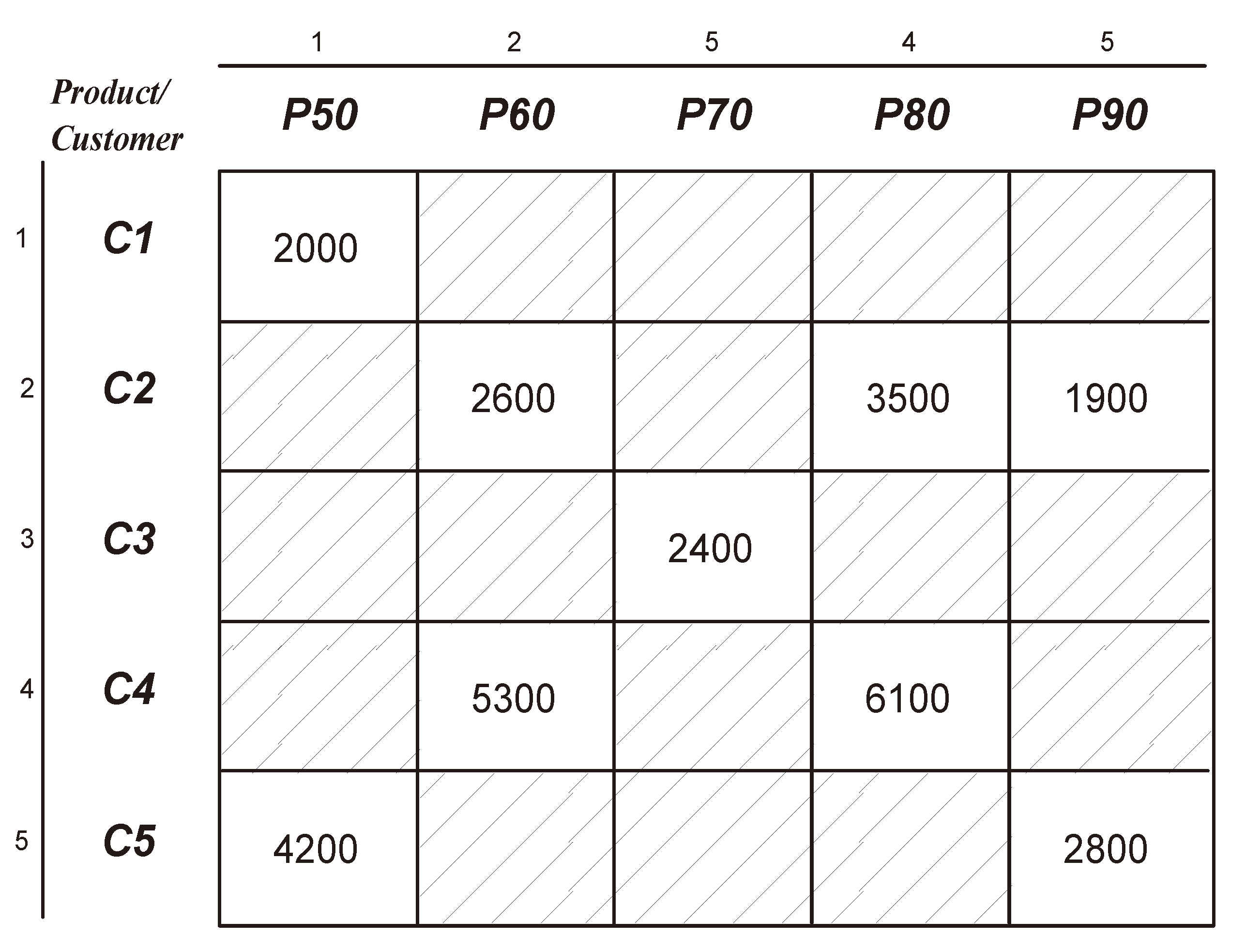
In this section, we detail the bitmap compression method used in MOLAP by presenting a simplified example consisting of a two dimensional array. The dimensions representing the indexes of this array are respectively products and customers, and the values represent sales amounts, each of which is a fact fora specific customer anda specific product.
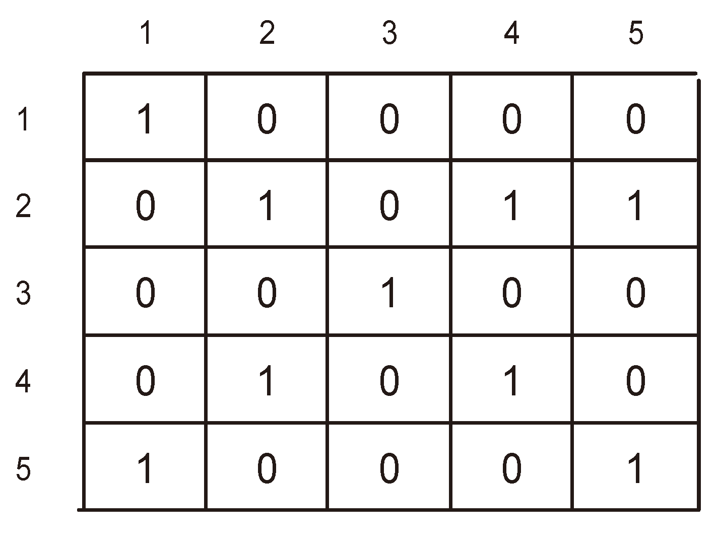
Figure 1 shows the original non-compressed matrix (two-dimensional array), in which null values are represented by dashed cells.
Figure 1.
Two-dimensional sparse matrix.
The bitmap compression scheme is using a bitmap multidimensional array (here a matrix of two dimensions for simplification) and a physical file vector that stores only the non-null values of a sparse multidimensional array [
4]. The role of the bitmap is to indicate the presence or the absence of non-null values in the original multidimensional array. In general, this technique is suitable for sparse data sets than for dense ones, so it can be largely used in OLAP systems.
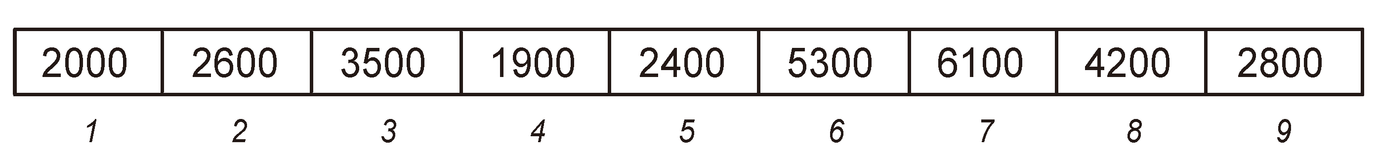
The bitmap compression starts by creating a multidimensional array of bits, which has the same number of dimensions as the original one, and another one-dimensional array called the value vector [
5], which stores the non-null values of the original multidimensional array. Therefore, for each cell in the original multidimensional array, if its value is null, then the corresponding value in the bit multidimensional array will be set to 0, otherwise it will be set to 1 and its measure will be added to the value vector (see
Figure 2 and
Figure 3). The basic method used to search a non-null value in the bitmap compressed structure consists of counting the number of values equal to one in the bitmap multidimensional array by traversing the cells starting from the first up to the corresponding searched value position. Once counted, their count result is used as the index of the non-null searched value in the value vector.
Figure 2.
Generated bitmap matrix corresponding to
Figure 1.
Using this bitmap compressed structure, the null values can be put away from any processing and only non-null values will occupya complete storage space.
For example, the sales of customer
C4 of product
P70 is null as
cell(4,3) = 0 (
Figure 2). But, the sales of
C4 for product
P80 is not null as
cell(4,4) = 1 (
Figure 2). To locate the corresponding sales amount in the compressed bitmap structure, we have to count the number of 1s starting from the first cell up to
cell(4,4) included. The count can be calculated by summing the implied cells such as
cell(1,1) +
cell(2,2) + ... +
cell(4,4) = 7, which means the corresponding sales amount value can be accessed directly at the 7th index of the value vector (
Figure 3), which contains the value
6100 matching the sales amount of customer
C4 for product
P80 in the non-compressed structure (
Figure 1).
3. Using Binary Search Tree to Store Compressed Data
Many algorithms based on the use of different tree structures were proposed for storing or indexing the data cube [
6,
7]. We propose an algorithm based on the bitmap compression method combined to the binary tree data structure. This algorithm starts by calculating a multidimensional array of bits to represent the existence of data elements in a sparse multidimensional data cube. The generation of the multidimensional array of bits is the same as in the bitmap method (
Figure 2). However, compared with the classical bitmap method, instead of using the value vector of bitmap method (
Figure 3), we use a binary search tree (BST) [
8] data structure to store the compressed data instead of the linear value vector used in bitmap.
A binary search tree is a binary tree in which each internal node
x stores a value such that the values stored in the left sub-tree of
x are less than or equal to
x and the values stored in the right sub-tree of
x are greater than
x [
9].
To adjust the binary search tree structure to store and maintain the data of a multidimensional array, we introduce the following two algorithms for inserting and searching values in the adapted binary search tree structure. To be able to make the mapping between the cells of the multidimensional array of bits created at the first bitmap phase and the data location within the binary search tree, we use the original indexes—instead of the value—of the data element in the multidimensional data cube as a traversal guide in the BST.
Therefore, the adapted binary will be organized as a binary tree, in which each internal node x stores a value such that the values stored in the left sub-tree of x have indexes in the original multidimensional data cube that are less than the indexes of x, and the values stored in the right sub-tree of x have indexes in the original multidimensional data cube that are greater than the indexes of x. Each node x of the tree will store, in addition to the value, a vector containing the indexes of this value in the original multidimensional cube. The vector size is static and equal to the dimension of the matrix representing the multidimensional cube. A more compact indexing method can be used to replace the vector of indexes in order to guide the traversal of the binary tree. This indexing method will be based on the observation introduced in the next section.
3.2. Inserting a Cell Value into the BST
This algorithm is used to insert the values of the multidimensional cube into the BST. Each value has to be inserted in the BST according to its key index ki.
Therefore, a node of the BST will store, for each non-null multidimensional cube cell, the pair constituted by the value v contained at this cell and its key index ki. The parameters of the recursive algorithm “insert” include the value v, its key index ki and a node initialized to the root of the BST at each call. The algorithm creates a new node for v by inserting it in addition to its key index into that new node when a null node pointer is reached (e.g., if the root is null, v will be inserted as a root). Before the null node pointer is reached, the algorithm will recursively call its right child node or its left child node and test the key index ki of the value v. It will go right if v is greater than the key index of the visited node and go left if otherwise. Note that the key index of the inserted value cannot be equal to an existing key index in the BST, as each key index represents a different cell in the multidimensional cube.
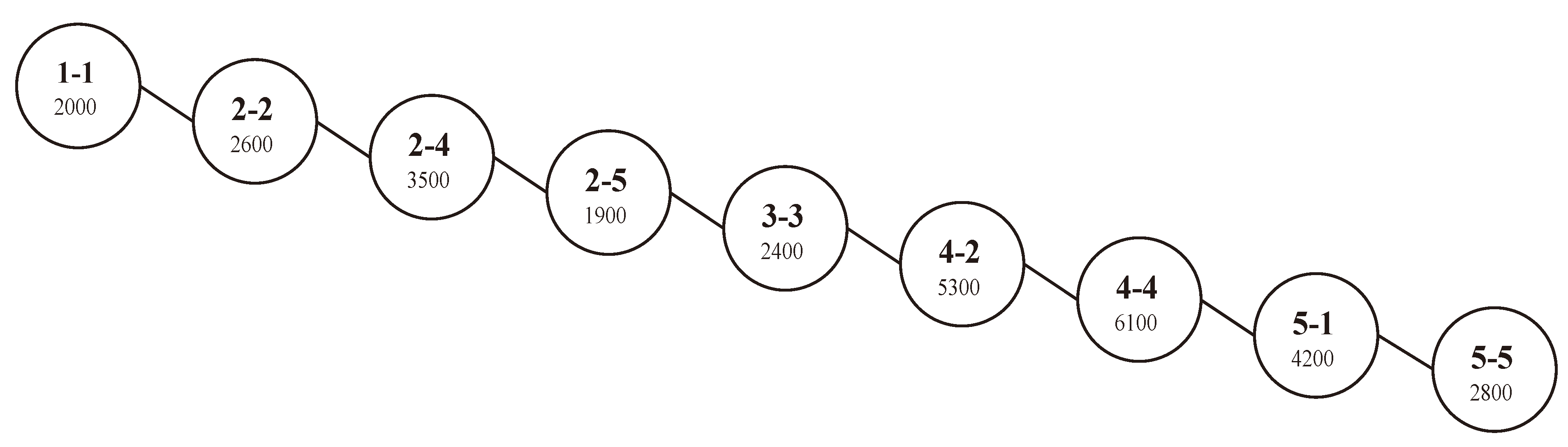
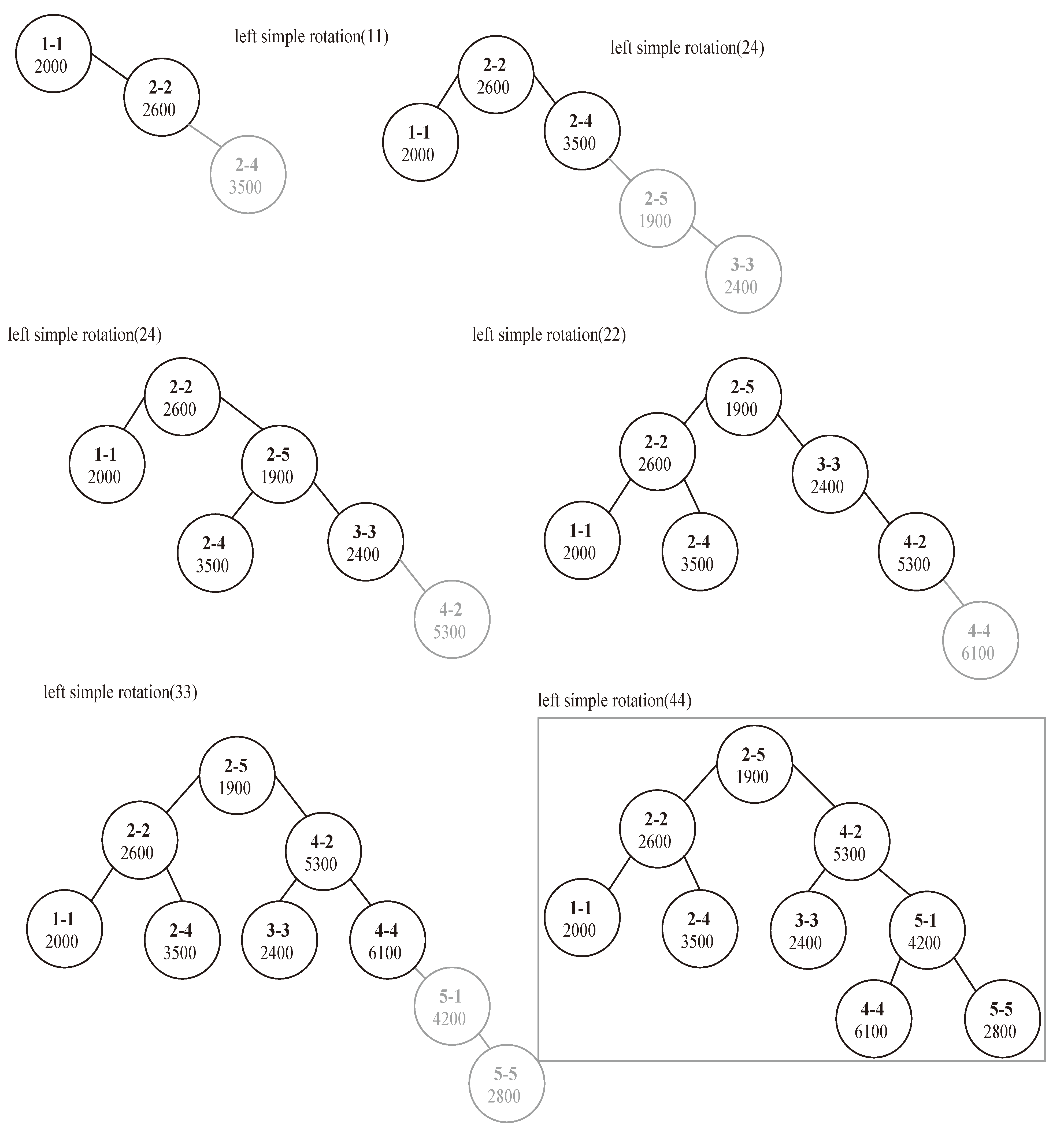
For example, we will show the result of applying of the “insert” algorithm to the values stored in the matrix of
Figure 1. The values of this matrix will be inserted sequentially in the data cube as in a real world application where the sequence of inserting is the sequence of data arrival from the loading process, in which facts are added as new values to the end of the multidimensional cube. Each non-null value from the sparse matrix (
Figure 1) has to be inserted into the BST. We start by the fact value
v = 2000 of
C1,
P50, which occupies the cell [1,1] on the matrix, so its key index
ki =1 − 1. This pair of data (
v = 2000,
ki =1 −1) will be stored in new node representing this cell in the BST. As the tree is empty, the corresponding node will be inserted as a root without further processing (see
Figure 4). The next non-null fact value
v = 2600 in the matrix matches the dimensions
C2,
P60, which has a key index
ki = 2 − 2. The index of the cell is 2 − 2 > 1 − 1 (the index of the root) and thus the new node for the pair (
v = 2600,
ki =2 −2) needs to be inserted to the right of the root. Afterward, new nodes will be created respectively for the pairs (
v,
ki) as in
Figure 4 having the values (3500, 2 − 4), (1900, 2 − 5), (2400, 3 − 3), (5300, 4 − 2), (6100, 4 −4), (4200, 5 − 1) and (2800, 5 − 5) [
11].
Figure 4.
Binary search tree corresponding to the matrix of
Figure 1.
The search in the BST is done according to the value of the key index. Like the insert algorithm, the search algorithm compares the key indexes to know the direction to be followed in order to retrieve the searched value.
3.3. Searching a Cell Value in the BST
The search algorithm takes as first parameter a key index ki, which represents the indexes of the searched cell (normally a cell that has a value “1” in the bitmap multidimensional array), and the current node “node”, which is initiated to the root at each external call. If the searched key index ki is found into a node in the BST, then the algorithm will return the value v from this node.
For example, the value at position [2,4] in the bitmap matrix of
Figure 2 is
1. Thus, to locate the original value, we apply the search algorithm using
204 as actual parameter for
ki. The algorithm will return the value
v = 3500 from the node having
ki =2 − 4, which corresponds to the original value at position [2,4] in the two-dimensional sparse matrix of
Figure 1.
Applying the search for a value in the BST structure can be done in a logarithmic time in the best case depending on the size of the problem
n (number of non-null value in the multidimensional array), which is better than the linear time requested by the bitmap search. However, the BST can become unbalanced as in our example in
Figure 4, which leads to a linear time complexity in the worst case. Thus, the proposed algorithm will be at the same complexity level in the worst case as the classical bitmap search algorithm.
3.4. Balancing the Tree to Reduce the Time Complexity
To overcome the lack of time complexity in the worst case scenario, we choose to use a balanced binary search tree instead of a classical one. For this reason, we choose the AVL tree structure [
12]. Inserting a node into an AVL tree is a two-part process. First, the item is inserted into the tree using the usual method for insertion as in a binary search tree. After the item has been inserted, it is necessary to check that the resulting tree is still balanced. A tree is considered balanced if for any node of this tree the height of its left sub-tree differs from the height of its right sub-tree by at most one level. This difference is called the balance factor of that node. When the tree becomes unbalanced, a single or a double rotation to the left or to the right has to be applied to the tree in order to re-balance it.
A single rotation to the left means rotating from the left toward the right. The right child of a node is rotated about it. In other words, the node becomes the left child of its right child. A single rotation to the right is done in the other way; the node becomes the right child of its left child (symmetric to the left rotation).
A double rotation can be regarded as a combination of left and right single rotations. A double left rotation at a node can be defined to be a single right rotation at its right child followed by a single left rotation node itself. Rotations are done symmetrically for the double right rotation.
By keeping the tree balanced, we can maintain a time complexity of
O(log(
n)) search capability even in the worst case. For that, an additional test for the balance factor has to be added to the inset algorithm (in
Figure 4) and one of four rotation functions has to be called when |
balancefactor|≥ 2 (which means that the tree is not an AVL).
Remarks:
Figure 5.
Balanced BST corresponding to the matrix of
Figure 1.
4. Incremental Hashing
In [
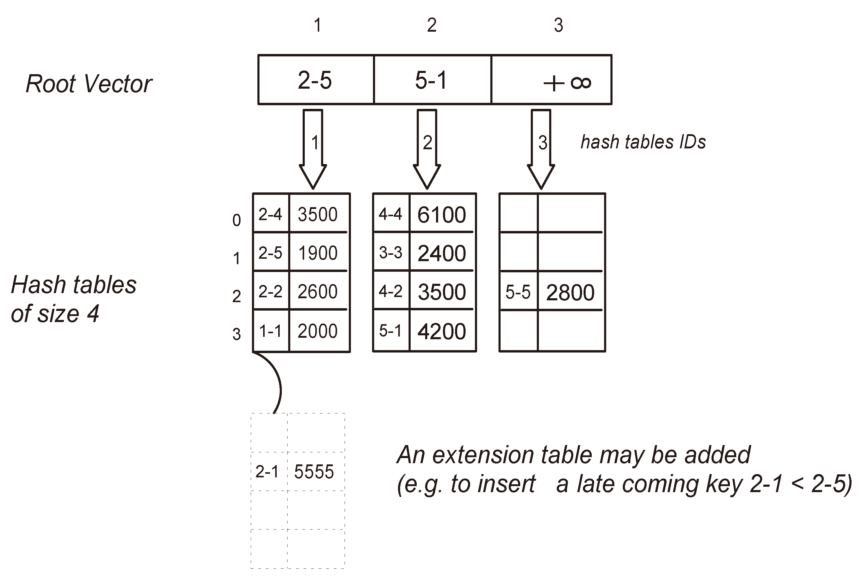
15], a novel compressed bitmap index approach is proposed, which reduces CPU and disk loads by introducing a reordering mechanism based on the locality-sensitive hashing (LSH). Furthermore, combining bitmap compression and hashing storage techniques can be useful for reducing space and accelerating the query response as it has been demonstrated. Our intension to profit from the advantage of this combination leads us to use the compressed bitmap schema to incrementally generate fact indexes and then to use them to insert and locate fact data in a dynamic hash structure. We start by creating a collection of hash tables having the same size. The generation of these tables will be done incrementally in a way that when the existing tables become full, one new table will be automatically created to allow the insertion of new keys. A vector containing critical key indexes will be used as a root of the proposed data structure to handle the insertion of keys into the corresponding hash tables and the search of the keys within the hash tables. This vector will play the role of an interface that guides the access to the concerned hash tables in order to minimize the time complexity of insertion and search operations (see
Figure 6). On the other hand, the goal of the incremental creation of hash tables is to minimize the space complexity of the used data structure, as only one small-sized hash table will be created and maintained at a time instead of a single huge-sized one that reserves empty null-valued cases. Consequently, the limited small size of hash tables will minimize the time complexity needed for handling the collisions that can happen during the insertion into these tables.
Figure 6.
Structure of incremental hashing.
4.1. Handling the Operations
Initially the root vector will contain only one value, which is the infinity, and it will point to an empty hash table of size m.
4.1.1. Insert Operation
Inserting data will always take place into the hash table pointed by a critical key that is greater than or equal the key index of the data to be inserted. The initial and last cell value of the root vector will be always the infinity value. This insertion method will generate values in the root vector in ascending order, where each value of this vector will finally point to a hash table containing keys less than or equal to it.
After locating the insertion point of a value in the corresponding hash table, a closed hashing method is applied over the key index to solve the collisions and to find an available empty cell in which the key index and its related data element value from the multidimensional cube have to be inserted. To simplify our tests, we used the linear probing as a closed hashing method, but other methods can be used such as the double hashing in order to avoid the primary clustering problem that can happen with the former method.
When the pointed hash table becomes full, the maximum value among its key indexes will be returned back to the root vector and placed in the cell pointing to this hash table that was originally pointed by the infinity value. Subsequently, the infinity value will be shifted up to a new cell just after the newly inserted maximum key index. Finally, a new hash table of size m will be created to allow new insertions. This process will continue as long as new non-null-valued cells are loaded into the MOLAP cube.
In order to keep the ascending ordering of the root vector adequate, we allow the creation of extension hash tables (of the same size m) that will be pointed by the corresponding full hash table to be extended. This can happen when the insertion point of a late incoming key index is located at a full hash table.
4.1.2. Search Operation
To search a value having a key index
ki, the search will start into the root vector by comparing the value of the index key consecutively with the values of the root vector until reaching a value greater than or equal
ki [
16]. In the worst case, the last infinity value will be greater than
ki. Once this greater or equal value is found, the hash table pointed by its case (numbered as its index) will be elected as containing the searched key. Thus, the search will take place only into this hash table of size
m and probably in its extensions if they exist. The same hash method used during insertion will be applied in order to find the key location within the elected hash table.
According to our proposed indexing properties (see
Section 3.1) and the previous insertion algorithm, the searched key index cannot be found in another table if it has not been found in the elected one or its extensions, because the key indexes are supposed to be inserted in the ascending order of the root vector. This search strategy also facilitates the search of a range of keys in a way that a subset of hash table most likely adjacent will be elected as containing the keys of the range interval and the search will take place only within this subset. The root vector has a size of
k, which is proportional to the number of key indexes
n currently existing in the multidimensional cube and the fixed size of hash tables
m, such that
k ≈ n/m + 1, by ignoring the extension tables, which are in fact rare.
Remarks:
(1) The time complexity of operations in the worst case is:
(2) In the average and best cases the time complexity is constant O(1).
5. Empirical Results
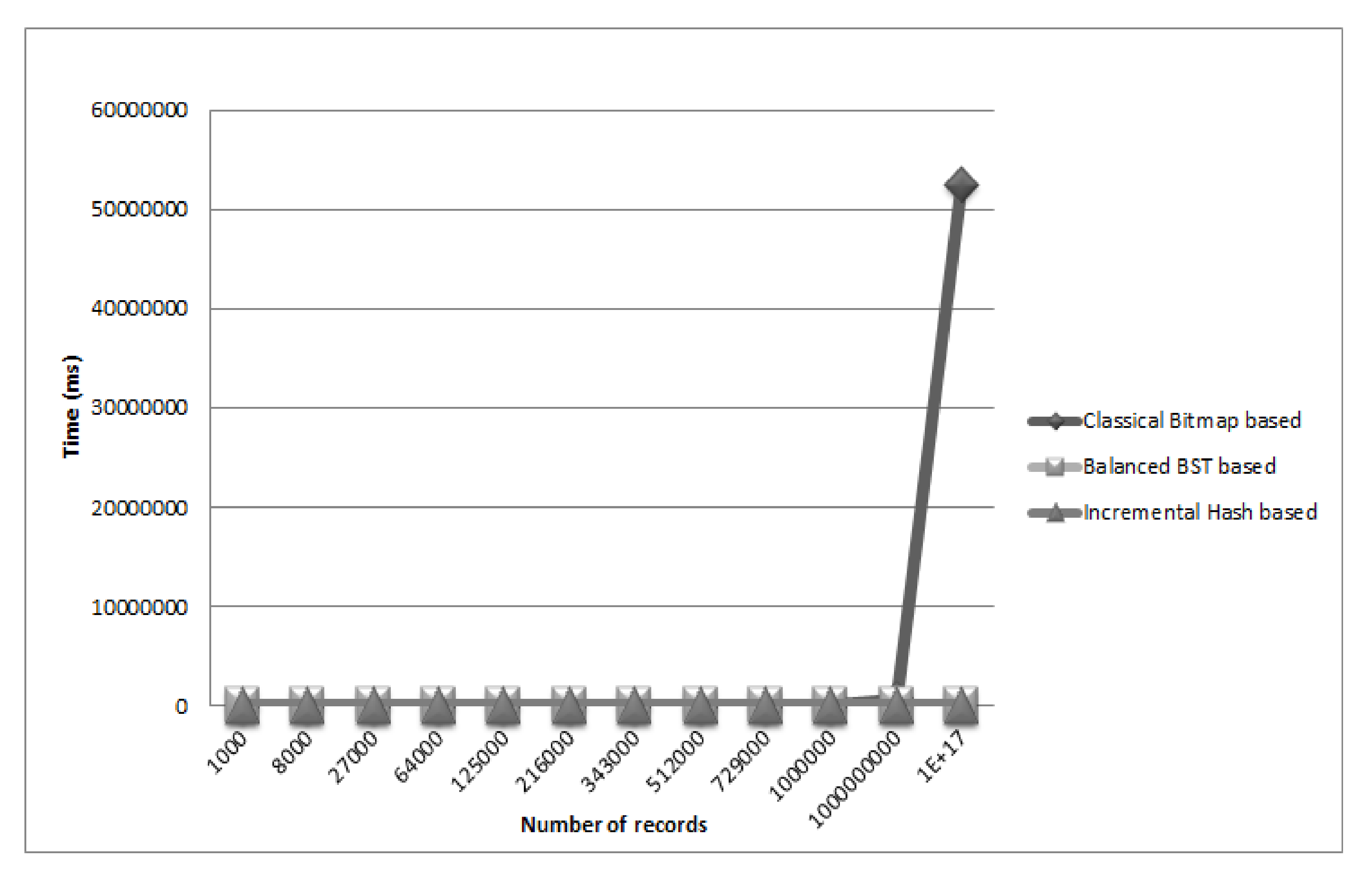
In this section, we show some empirical results obtained by running prototypes of our algorithms written in C++ language and the classical bitmap algorithm over a number of data sets. Each chosen data set represents a data cube (three-dimensional array). The number of facts (null or not) in the cube is represented in the first column of
Table 1. The sparsity in all cubes is about 20%. The last three columns of the table represent respectively the running time in millisecond for the classical bitmap algorithm, for the balanced BST based algorithm and for the Incremental Hash based algorithm.
Figure 7 represents graphically the difference in running time among the three algorithms while searching for data. According to the obtained result, the algorithms based on BST and Incremental Hash dramatically outperform the classical bitmap, especially when the number of cells increases above 1,000,000,000. Besides, the Hash based algorithm performs faster than the BST based algorithm when the data size increases.
Table 1.
OLAP Search time comparison.
| 3-D cube size | Classical Bitmap | Balanced BST | Incremental Hash |
|---|
| (Number of cells/facts) | Time (ms) | Time (ms) | Time (ms) |
|---|
| 103 = 1000 | 17.1 | 16.21 | 15.24 |
| 203 = 8000 | 53.73 | 17.28 | 16.98 |
| 303 = 27,000 | 168.2 | 19.88 | 19.34 |
| 403 = 64,000 | 328.4 | 21.63 | 21.67 |
| 503 = 125,000 | 653.6 | 26.47 | 24.81 |
| 603 = 216,000 | 993.2 | 30.01 | 27.12 |
| 703 = 343,000 | 1394 | 34.12 | 31.23 |
| 803 = 512,000 | 2570 | 50.76 | 35.22 |
| 903 = 729,000 | 3047 | 69.20 | 40.03 |
| 1003 = 1,000,000 | 59,911 | 155.31 | 46.52 |
| 10003 = 1,000,000,000 | 600,054 | 232.01 | 70.39 |
| 1016 | 52518054 | 2120 | 1412 |
Figure 7.
Running time comparison.
For all the tested benchmarks, the compression ratio was proportional to the sparsity of the cube. For 20% of sparsity the compression ratio was 18.4% and 24.18% depending on the size of the cube [
17], and for 40% sparsity it was 39.16% and 46.34%.
6. Conclusions
In this paper, we adapted multiple data structures that can store multidimensional arrays (hypercubes) in a way to eliminate the sparsity of these arrays and to accelerate the search process within their data contents. Several methods have been recently developed for compressing data cubes in MOLAP systems and some others for speeding up the query processing. Our objective was to combine these two tasks by using convenient data structures that can serve to compress the data and to optimize the operations over them without the need for decompression. We proposed a new compact indexing strategy that can be easily calculated and then retrieved directly from the uncompressed hypercube structure. This indexing strategy has been subsequently used to identify the data elements in two different compressed data structures. The first compressed structure consists of using the classical bitmap technique by creating a multidimensional cube of bits having the same number of dimensions as the original uncompressed hypercube, but it replaces the single dimension array used to store the non-null values by a balanced binary tree (i.e., the AVL tree), in which the nodes are inserted and later searched depending on their compact indexes (which are calculated according to their indexes of cells in the original uncompressed hypercube) instead of their values. This chosen structure allows to search within compressed data in logarithmic time instead of the linear time required for searching in a classical bitmap compression structure. The second compressed structure is based on hashing, in which multiple hash tables of a limited prefixed size are created dynamically on demand, one after another and maintained by a vector containing a subset of critical compact indexes. This later allows speeding up the search in the proposed structure and consequently the other operations such that the insertion will be also accelerated as its acceleration is based on the speed of the search operation. On the other hand, the limited size of the hash tables allows the reduction of time needed to handle the collisions that can happen in these tables. This structure requires a time complexity that varies from logarithmic in the worst case for all the operations to constant in the average and the best cases. The incremental hash algorithm requires less execution time as well as less space to maintain its structure compared with the balanced tree based algorithm. Our perspective is to try additional data structures that can serve for data compression always by using our proposed compact indexing strategy. As a tactical objective, we will try to use the compact indexes to serve as clustered indexes for records containing the facts as attribute values. We think that this structure will be beneficial when a query tries to retrieve some interval of index values, as the input/output operations will be reduced due to the physical order of data stored at each disk block.


