Abstract
Due to the increasing harmfulness of software vulnerabilities, it is increasingly suggested to propose more efficient vulnerability assessment methods. However, existing methods mainly rely on manual updates and inefficient rule matching, and they struggle to capture potential correlations between vulnerabilities, thus resulting in issues such as strong subjectivity and low efficiency. To this end, a vulnerability severity assessment method named Latent Space Networks (LSNet) is proposed in this paper. Specifically, based on a clustering analysis in Common Vulnerability Scoring System (CVSS) metrics, we first exploit relations for CVSS metrics prediction and propose an adaptive transformer to extract vulnerability from both global semantic and local latent space features. Then, we utilize bidirectional encoding and token masking techniques to enhance the model’s understanding of vulnerability–location relationships, and combine the Transformer method with convolution to significantly improve the model’s ability to identify vulnerable text. Finally, extensive experiments conducted on the open vulnerability dataset and the CCF OSC2024 dataset demonstrate that LSNet is capable of extracting potential correlation features. Compared with baseline methods, including SVM, Transformer, TextCNN, BERT, DeBERTa, ALBERT, and RoBERTa, it exhibits higher accuracy and efficiency.
1. Introduction
As digitalization continues to advance, software vulnerabilities have become increasingly prominent. The International Business Machines Corporation (IBM) “2024 Cost of a Data Breach Report” [1] indicates that the average cost of data breaches, primarily caused by software vulnerabilities, has reached 4.88 million USD, resulting in a growing severity of economic losses. Pan et al. [2] propose that a strategy gaining traction is to detect new software vulnerabilities by analyzing related development activities, which facilitates timely alerts for open source software users. Consequently, in both enterprise economic activities and the process of users utilizing software, accurate and efficient vulnerability severity assessment is becoming increasingly significant. However, traditional vulnerability assessment methods predominantly rely on manual updates and inefficient rule-matching approaches [3]. These methods suffer from inherent limitations such as high subjectivity and inefficiency, rendering them inadequate for addressing increasingly complex cybersecurity threats.
In recent years, intelligent analytical approaches represented by machine learning algorithms have emerged as a research focus, including classification-based methods like Markov models [4], Support Vector Machines (SVM) [5], K-Nearest Neighbors (KNN) [6], and clustering-based methods like K-means cluster [7]. For example, Zheng et al. [6] proposed a KNN-based vulnerability exploitability assessment method. This approach pioneered a network environment-oriented evaluation framework and introduced a group expert–statistical dimensionality reduction paradigm for indicator selection, significantly enhancing assessment accuracy and effectiveness. However, most machine learning models depend on high-quality human-annotated data. For example, Microsoft proposes a “risk matrix” methodology to determine the severity levels of software vulnerabilities [8,9]. Vulnerability severity labeling necessitates both theoretical analysis and practical attack validation. Consequently, these methods exhibit constrained performance boundaries and limited generalizability when confronted with multi-source, heterogeneous, dynamically evolving vulnerabilities and complex threat scenarios. Additionally, they demand substantial domain-specific expertise. Currently, with the rise of deep learning technology, its capacity to autonomously learn deep-seated features of data through multilayered nonlinear networks offers a new paradigm for overcoming the performance constraints of traditional machine learning in vulnerability severity assessment. Compared to shallow machine learning models reliant on manual feature engineering, deep learning models like Convolutional Neural Networks (CNN) and their variants [10,11], as well as Recurrent Neural Networks (RNN) [12], significantly enhance automation and precision in complex scenarios.
Despite their success, the current paradigm faces critical limitations: it struggles to maintain high accuracy when processing highly specialized, domain-specific vulnerability descriptions characterized by intricate semantics, substantial information density, and urgent demands for rapid assessment [13]. Likewise, it is still not feasible to conduct vulnerability severity assessments in a fully automated and highly efficient method. Specifically, vulnerability data frequently suffer from noise interference and sparse critical features [14], while single deep learning models used for vulnerability assessment exhibit limitations in extracting composite features of critical vulnerabilities [15], as represented within Figure 1a.
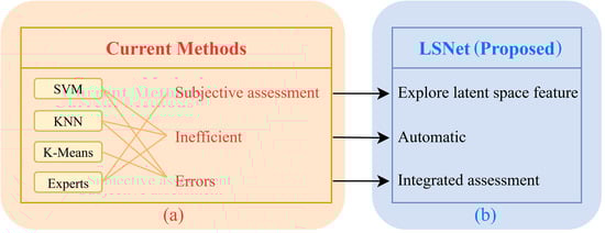
Figure 1.
(a,b) Comparison between the current methods and LSNet.
To address these flaws, we propose a vulnerability classification model integrating clustering feature analysis and Transformer architecture by combining cluster analysis, the BERT pretrained model, Transformer structures, and TextCNN modules. The model decomposes vulnerability severity assessment into eight submodels, each responsible for classifying specific metrics within the Common Vulnerability Scoring System (CVSS) vector string. Initially, the pretrained BERT model generates word vectors from cleaned vulnerability text data. Subsequently, explicit and implicit textual features are fused through bidirectional encoding and token masking modules. The Transformer’s self-attention mechanism and convolution modules then extract global and local features from the vulnerability descriptions. Finally, the model jointly trains global and local latent space features alongside explicit and implicit information to enhance classification performance. The classification results are concatenated to form the CVSS vector string, from which the CVSS scores are calculated to determine vulnerability severity levels. This severity assessment serves as the basis for evaluating vulnerability threats, thereby enabling timely countermeasures. Its advantages are illustrated in Figure 1b. The main contributions of this paper are as follows:
- (1)
- We propose a novel vulnerability severity assessment model named LSNet, which handles longer textual information and extracts more effective latent associations features from vulnerability descriptions.
- (2)
- We perform feature extraction through clustering to enhance latent associations within the text. Subsequently, we propose bidirectional encoding and token masking to strengthen the model’s comprehension of textual semantics, and integrate the Transformer method with convolution to extract vulnerability text features, significantly enhancing the model’s capability to identify vulnerability texts.
- (3)
- Experiments conducted on NVD and CCF OSC2024, supplemented by vulnerability density fitting curves, demonstrate the highest accuracy of 97.1% and average mean squared error improvements of 11.16% in vulnerability severity assessment tasks compared to prior state-of-the-art vulnerability severity assessment methods and baseline models.
The rest of this paper is organized as follows. Section 2 discusses existing work on vulnerability severity assessment. Section 3 introduces the proposed model methodology, highlighting the innovation and rationale of this work. Section 4 discusses experiments and data analysis, presenting the dataset, testing environment, and comparative performance of model metrics, along with a detailed error analysis and ablation studies to comprehensively validate the method’s effectiveness. Section 5 concludes the paper and outlines future research directions. Similarly, we produce a table to summarize the key abbreviations used throughout the paper, as shown in Table 1:

Table 1.
Table of key abbreviations.
2. Related Work
In this section, we will first introduce the background of the creation of the CVSS, and then review the latest progress in the current state-of-the-art vulnerability severity assessment work and vulnerability severity assessment methods.
2.1. Common Vulnerability Scoring System
The Common Vulnerability Scoring System serves as a critical evaluation framework in information security, playing a pivotal role in quantifying vulnerability threats. Developed by the National Infrastructure Advisory Council (NIAC) and maintained by the Forum of Incident Response and Security Teams (FIRST), this system introduces standardized metrics to classify vulnerability severity, providing objective foundations for risk management [16]. It has gained widespread application in vulnerability prioritization, compliance auditing, and enterprise information security maintenance, establishing itself as the benchmark for modern vulnerability management ecosystems. The metrics comprise three key scores: the Base Score (BS), Exploitability Score (ES), and Impact Score (IS), and they can be used to quantify vulnerability severity [17]. These scores collectively measure: (1) vulnerability characteristics throughout the lifecycle; (2) domain-specific network security threats; and (3) potential impacts on end-users [3]. Derived from CVSS vector strings, these metrics are primarily determined by subject matter experts based on established evaluation criteria. The National Vulnerability Database (NVD) assigns standardized severity assessments for each vulnerability within its public repository, known as the Common Vulnerabilities and Exposures (CVE) list. This scoring methodology comprehensively considers exploitability, impact scope, attack complexity, and other factors, and is widely used and extensively adopted for vulnerability threat prioritization. While the system offers significant advantages in facilitating vulnerability prioritization, such as providing objective risk quantification, it has inherent limitations, including its limited adaptability to dynamic attack vectors, low automation level and excessive reliance on domain experts for manual judgment. Consequently, this paper concentrates on quantification gaps within specific vulnerability lifecycles, introduces an innovative analysis pathway incorporating comprehensive threat modeling to enhance precision in risk identification, and constructs a fully automated vulnerability assessment system based on CVSS3.1.
2.2. K-Means Clustering Based Vulnerability Severity Assessment
K-means clustering plays a crucial role in feature extraction. This algorithm partitions high-dimensional vulnerability data into K clusters by minimizing within-class variance, thereby revealing common patterns and shared characteristics of vulnerability exploits [18]. Applied in vulnerability detection, it offers a superior alternative to traditional rule-based feature analysis methods. K-means effectively captures feature data, such as code similarity, memory access patterns, and dynamic behaviors across vulnerabilities. This capability enhances the model’s comprehension of latent relationships between vulnerability descriptions and their corresponding threat levels [19,20]. The current framework of vulnerability clustering approaches primarily focuses on analyzing latent correlations among vulnerabilities, thereby neglecting essential dimensions required for comprehensive severity assessment, leading to suboptimal classification outcomes. Thus, this study bridges this gap by leveraging transformer technology to integrate clustering features with severity analysis mechanisms.
2.3. Transformer Model
Vaswani et al. [21] introduced a Transformer encoder–decoder architecture based on the self-attention mechanism, offering a novel solution for vulnerability severity assessment. This framework abandons the sequence modeling paradigm of traditional recurrent neural networks (RNNs), employing a structure solely based on the attention mechanism to model global dependencies in input sequences [22]. The model significantly enhances parallel processing capabilities and long-range dependency capture through multi-head attention and feed-forward neural networks. For vulnerability severity assessment tasks, the Transformer encoder–decoder architecture effectively handles long-distance dependencies and complex semantic structures within vulnerability description texts. The self-attention mechanism enables the model to dynamically focus on critical vulnerability features, while multi-head attention concurrently captures global contextual representations, thereby extracting holistic characteristics of vulnerability texts and identifying intricate patterns within them [23,24]. Previous Transformer-based vulnerability severity assessment models still fail to integrate underlying correlations because the models ineffectively capturing latent dependencies between vulnerabilities. Building on that basis, this paper integrates feature biases derived from K-Means clustering to optimize the vulnerability classification model. By incorporating clustering patterns into the Transformer framework, the approach enables the model to assimilate both explicit dependency relationships and latent cluster characteristics, thereby achieving enhanced assessment accuracy for vulnerability severity levels through multi-dimensional feature fusion. This integration strategy significantly advances beyond conventional single-model solutions.
3. Method
In this paper, we propose a vulnerability severity assessment model integrating clustering feature analysis and the Transformer method, which comprises four hierarchical layers, depicted in Figure 2. First, the word-embedding layer processes vulnerability information text through data cleaning and lexical preprocessing, converting tokens into node vectors. This layer incorporates bidirectional text encoding and token masking mechanisms to enhance the positional awareness of Common Vulnerability Scoring System vector strings [25]. Secondly, the TextCNN-based [26] feature extraction layer captures local textual patterns while integrating clustered features. Third, the Transformer-TextCNN feature fusion layer amalgamates vulnerability characteristics extracted via clustering, further strengthening the model’s positional sensitivity to vector strings. Finally, the fully connected output classification layer synthesizes distributed features, generates one-hot probability distributions, and ultimately produces predicted classification.
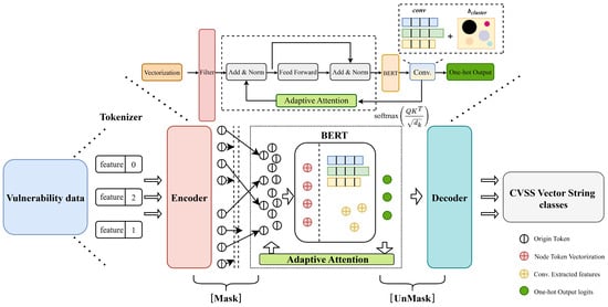
Figure 2.
Model architecture of LSNet.
3.1. Clustering Feature Analysis
In this paper, we propose clustering-based data mining analysis as its foundational motivation, uncovering a novel method for predicting CVSS scores. It utilizes the results of clustering feature analysis as feature weights during model training.
Given the complexity of raw textual data, dimensionality reduction becomes essential for processing the extracted features from Common Vulnerabilities and Exposures vulnerability text. Principal Component Analysis (PCA) [27] serves as the dimensionality reduction technique, with empirical findings indicating optimal performance at two dimensions. This approach sufficiently preserves feature integrity while significantly streamlining data complexity [28]. Subsequent standardization processing enables the revelation of latent vulnerability behavioral patterns within the data. The methodology involves in-depth analysis of textual information through the CVSS framework to examine inter-component relationships across vulnerability elements. K-Means clustering then excavates underlying threat patterns from this analysis. Simultaneously, a postulated Gaussian Mixture Model investigates Gaussian distributions across vulnerability datasets, simulating vulnerability propagation dynamics throughout their lifecycle evolution [29].
The desired outcome for each cluster is maximized intra-cluster similarity and minimized inter-cluster similarity. To quantify cluster separability, this methodology introduces Minkowski distance measurement
and cosine similarity assessment
as dual quantitative metrics.
In the formula above,
denotes the lateral separation distance between clusters,
is the defined dimensionality and
is the order of distance, while
represent the horizontal and vertical separation distance.
By integrating the following three comparative methods and applying the elbow criterion, it is possible to determine an effective combination of dimensionality reduction parameters and cluster count [30]:
(1) Sum of Squared Errors Criterion: A smaller sum of squared errors indicates better clustering performance, which measures the predictive accuracy of a model by calculating the sum or average of squared differences between predicted and actual values, as follows:
where
denotes observed values and
represents predicted values, followed by summation over all samples. This formula quantifies the discrepancy between predicted and observed values.
(2) Silhouette Coefficient: This metric evaluates the impact of different algorithms or algorithmic configurations on clustering results using identical raw data and quantifies how well each data point fits into its assigned cluster relative to other clusters. Normalized within [−1, 1], values closer to 1 signify superior intra-cluster cohesion and inter-cluster separation.
Specifically,
measures the cohesion of a sample point, where
denotes other samples within the same cluster as sample
, and distance computes the distance of
.
is computed similarly to
, but requires iterating through other clusters to obtain multiple values, with the minimum selected as the final result. A smaller
indicates tighter cluster cohesion.
(3) Calinski–Harabasz Index: Defined as the ratio of between-cluster dispersion to within-cluster dispersion and quantifying the compactness and separation of clusters by calculating the ratio of between-cluster variance to within-cluster variance, where higher values denote better clustering outcomes.
where
represents the Calinski–Harabasz Index.
denotes the between-cluster scatter matrix, reflecting dispersion among cluster centroids, while
is the within-cluster scatter matrix, indicating dispersion among samples within the same cluster.
indicates the total number of vulnerability data points, and k represents the number of clusters.
However, considering practical constraints, excessively low dimensionality reduction may lead to an insufficient data volume in some clusters. Therefore, we select a configuration of 2-dimensional reduction with 4 clusters, which significantly mitigates the sample distribution imbalance issue [31]. The resulting clustering outcomes are visually presented in Figure 3, where the x-axis represents the first principal component, and the y-axis represents the second principal component. Principal components are linear combinations of all original features. The first principal component (PC1) indicates the direction that maximizes data variance, while the second principal component (PC2) is orthogonal to PC1 and explains the maximum remaining variance.
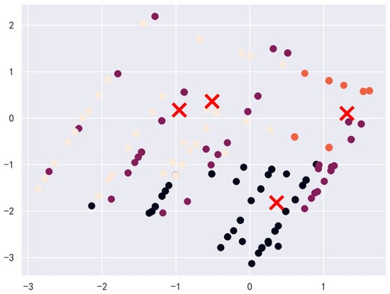
Figure 3.
Cosine similarity clustering analysis for vulnerabilities.
In this paper, we propose heatmap visualization to analyze the clustered data, examining the relationships and magnitudes of influence between individual metrics in CVSS vector strings and multidimensional CVSS scores. The heatmap illustrating the clustering analysis is depicted in Figure 4.
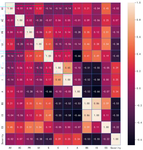
Figure 4.
Clustering analysis heatmap on CVSS metrics.
Consequently, the vulnerability severity assessment method proposed in this paper subdivides CVSS score prediction into eight distinct subproblems, each corresponding to individual metrics within the CVSS vector string [32]. By predicting outcomes for each metric, the approach synthesizes the predicted CVSS vector string, with the final CVSS scores thus calculated. This research designs a BERT-based deep learning model for CVSS scores prediction. The model separately trains and predicts each metric within the CVSS vector string, aggregates results, and consequently computes the CVSS scores for a given vulnerability instance.
3.2. Word Embedding
In this subsection, we elaborate on the word-embedding approach, covering data cleaning, initialization operations, encoding techniques, and the token-masking module to introduce the input data processing for LSNet’s training.
3.2.1. Data Cleansing
Before model training, data cleansing is essential to streamline the dataset and align it with task requirements. This paper adopts an approach to discard irrelevant columns such as “CVE-ID”, “Issue_Url_old”, “Issue_Url”, and “Repo_new” from the text information. Although potentially useful in other contexts, these features generally contribute minimally to vulnerability analyses or vulnerability correlation training. Consequently, retaining the vulnerability description text, CVSS vector strings, CVSS scores, and threat severity levels proves sufficient. For disordered vulnerability labels and irrelevant gibberish (e.g., “CVE_ID”:”CVE-2018-20847,” “description”:”Heap buffer overflow... NUMBERTAG ERRORTAG... URLTAG... NUMBERTAG”), regular expressions filter out erroneous terms and meaningless noise. Without this cleaning step, such artifacts would cause the model to fit noise and converge to a non-optimal solution.
3.2.2. Data Preprocessing
Preprocessing serves as a critical phase in natural language processing, transforming raw text into structured and standardized formats [33]. The subsequent clustering analysis suggested visualizing the processed data through heatmaps to examine relationships between individual CVSS v3.1 vector metrics and multi-dimensional CVSS severity scores. These visualizations reveal the contribution weights of each vector metric toward the final CVSS scores [34], reflecting their criticality in severity assessment. This preprocessing methodology enhances semantic comprehension for subsequent analytical models. Word preprocessing in our framework involves two sequential operations:
- (1)
- Stemming reduces words to their root forms, a technique widely applied in linguistic preprocessing. For vulnerability severity assessment, stemming extracts key terminology from vulnerability descriptions, simplifying feature expressions while boosting model convergence efficiency.
- (2)
- Lemmatization converts words to their canonical forms based on grammatical context. Unlike stemming, lemmatization accounts for syntactic roles, ensuring morphological standardization. In CVSS severity analysis, lemmatization strengthens the model recognition of polymorphic vulnerability-related terms. For instance, the words “attack” and “attacked” were grouped into identical lexical entries, minimizing interpretation ambiguities.
Our experiments use the Natural Language Toolkit (NLTK) for text preprocessing. Input vulnerability descriptions are first tokenized, then processed through NLTK’s Porter stemmer and WordNet lemmatizer modules. This pipeline standardizes lexical variations while preserving critical semantic indicators essential for transformer-based vulnerability classification.
3.2.3. Bidirectional Information Encoding
For vulnerability severity assessment tasks, transforming them into metric classification tasks for CVSS vector strings reveals that the sequence and relative position information of feature metrics play a decisive role in accurately parsing and determining vulnerability characteristics [35]. Given that encoding itself does not involve directionality, while bidirectional information is captured through model architecture, different orders of occurrence within the sequence often represent vastly different vulnerability configurations and severity implications. Thus, the proposed model first integrates an explicit bidirectional information encoding module, synergistically coupled with an implicit token masking mechanism at the subsequent layer. During word embedding of CVSS vector strings, the foundational Transformer model typically presents learnable absolute positional encoding to encode positional indices of each token in the sequence [36]. The resulting embedding vector matrix
contains position features implicitly acquired through internal model processing, primarily relying on absolute token indices [21,25]. However, this mechanism places greater emphasis on fixed sequential order, struggling to adequately model complex and critical functional dependencies and relative distance relationships among vulnerability metrics within vector strings, such as combinatorial effects between adjacent metrics or tight interconnections within specific metric groups.
To more effectively capture such inter-metric relative positional semantics embedded in CVSS vector strings, a bidirectional information encoding approach distinct from absolute positional encoding exclusively focused on fixed sequences is proposed. Beyond mere sequential order considerations, bidirectional information encoding can perceive forward and backward relative positional offsets between tokens, for example, the offset of metric AC relative to AV or C relative to I, while also offering inherent continuity and smoothness advantages [37]. Leveraging the periodic nature of sine and cosine functions, this encoding strategy enables the model to more robustly learn relative positional relationship features between any two metrics across varying distance scales, thereby significantly enhancing the comprehension of structured semantics in CVSS vector strings and improving classification accuracy for the metrics.
3.2.4. Token Masking
Token masking segments the string into minimal tokens to accurately localize specific indicator values for masking operations, thereby preventing the model from disrupting logical associations between labels and values and enabling the model to learn finer positional relationships in text [38]. This model utilizes the masked language modeling capabilities of BERT to implement token masking on CVSS vector strings. For the input CVSS vector string label
, we randomly mask and replace certain tokens of each indicator label with the special token [MASK] [25,39]. The model then predicts and recovers these masked tokens based on contextual information, leveraging vulnerability description text as input word vectors and the original CVSS vector string as the learning target label. This approach outputs classification results for each indicator in the CVSS vector string. The specific design of token masking is detailed in Figure 5.
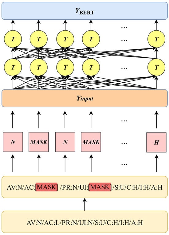
Figure 5.
Token masking encoding representation.
3.3. Transformer Adaptive Latent Space Feature Fusion
We propose LSNet, which integrates the self-attention mechanism of the Transformer method to capture global feature relationships within sequences, subsequently incorporating residual networks, layer normalization, and feed-forward networks to enhance model performance and training efficiency. For the transformer-encoded vulnerability text data
, the hidden states of the input sequence
(where
represents the sequence length and
denotes the hidden layer dimension) undergo linear transformations to generate query (), key (), and value () matrices as follows:
where
,
, and
, respectively, represent the query, key, and value matrices for the head, and
,
,
denote learnable weight matrices. We then use the following equation:
where
signifies the dimension of the key vector. Subsequently, we concatenate the attention scores
, obtained from h attention heads, and then multiply this concatenated result by the output projection weight matrix to obtain matrix
[21].
Then, TextCNN is used for feature extraction, where a textual description of vulnerability
is first passed through the convolutional layer to filter individual word vectors. The resulting vectors are then utilized as inputs to TextCNN. Using four adaptively sized convolutional kernels, the model extracts feature maps by performing convolution operations on the text sequence [26]. The resulting feature map sequences, denoted as
, incorporate the clustering vector association weights
obtained from Section 3.1 as convolutional bias, as illustrated below:
where
denotes vertical stacking, while
represents the convolution operation,
, determined by the optimizer. Leveraging TextCNN, we propose multi-channel, multi-kernel convolution operations on feature representation vectors generated by the Transformer encoder. This process extracts local commonality features across varying granularities of textual words and syntactic structures. Subsequently, maximum pooling is applied to achieve feature dimensionality reduction.
The pooled feature vectors are fed into the representation integration layer for classification operations and undergo nonlinear transformation via an adaptive activation function. The concatenated feature vector
is computed with the fully connected layer’s weight matrix
and bias term
.
where
denotes the weight matrix of the representation integration layer, and
represents the bias term that dynamically adjusts via adaptive attention mechanisms. The resulting
constitutes the nonlinearly transformed string feature vector.
The feature distribution
, after max pooling in the feature fusion layer, is input into a fully connected layer for classification, transforming it into a feature probability vector
. This vector undergoes normalization via the softmax function, enabling multi-class classification of each metric within the CVSS vector string to obtain their corresponding one-hot probabilities:
In this process, LSNet outputs the label value for each CVSS vector string. It applies the softmax function to determine the class with the highest probability, assigns a value of 1 to that class, and sets all other classes to 0, thereby obtaining the definitive label value for each CVSS vector string.
During experimental training, the model uses cross entropy as the loss function to quantify the discrepancy between predictions and ground truth labels. The Adam optimizer utilizes backpropagation to iteratively refine training parameters. This process progressively reduces classification loss while enhancing the model’s classification accuracy. The specific calculation for the cross entropy loss function is as follows:
where
represents the ground truth (GT) label,
denotes the total number of entries in the CVSS vector string, and
represents the model-predicted probabilities.
4. Experiment and Analysis
In this section, we comprehensively outline the overall framework for experimental design and result analysis. We first introduce the experimental setup and basic procedures. By comparing the performance of different models, we systematically assess the effectiveness of various methods. Furthermore, we combine multiple metrics and error analysis of prediction results to thoroughly investigate model behavior and limitations. Finally, we employ ablation experiments to validate the role of key components and their contributions to overall performance.
4.1. Dataset
To comprehensively validate the effectiveness of our proposed model for vulnerability severity assessment, we collected publicly available vulnerability data from the NVD (https://nvd.nist.gov/, accessed on 27 July 2025), spanning January 2018 to December 2024. After data preprocessing to remove entries with missing critical information, we obtained 126,607 valid entries. We randomly partitioned this corpus into training, validation, and test sets to form a large-scale dataset denoted as NVD throughout this paper. Additionally, we incorporated the vulnerability severity assessment dataset from the 7th China Computer Federation Open Source Competition (https://www.gitlink.org.cn/competitions/track4_vulnerability, accessed on 27 July 2025) as a small-scale dataset, referred to as the CCF OSC2024 in this paper (Table 2).
Table 2.
Statistics of datasets.
4.2. Experimental Setup
In this paper, all experiments employed identical environmental configurations. The operating system was Ubuntu 22.04 LTS, with an NVIDIA GeForce RTX 4090 GPU and Python 3.9 as the programming language. Deep learning models were built using PyTorch 2.5.0. Regarding hyperparameter selection, we refer to the original papers of BERT and TextCNN, employing the most commonly adopted initial learning rate, convolution kernel count and dimensions, convolution fusion layer parameters that demonstrated optimal performance for the classification task. The Adam optimizer dynamically adjusts the learning rate during training, with specific configuration details provided in Table 3.
Table 3.
Model parameter settings.
4.3. Evaluation Metrics
In this paper, we introduce quantitative methods to evaluate model performance and vulnerability severity assessment outcomes. For the classification results of CVSS vector string metrics generated by the model, samples are categorized into four types based on their ground truth labels and model predictions: correctly classified positive samples are true positives (TP), incorrectly classified positive samples are false positives (FP), correctly classified negative samples are true negatives (TN), and incorrectly classified negative samples are false negatives (FN). Based on these categorizations, the model’s accuracy (Acc), Precision, and F1 Score serve as evaluation metrics. The corresponding formulas are as follows:
Within the CVSS, the classification results of CVSS vector string metrics generated by our model undergo standardization through a computational formula, yielding normalized values within the [0, 10] interval. Consequently, this paper additionally adopts mean squared error (MSE) as a performance evaluation metric for the proposed vulnerability severity assessment method, thereby demonstrating its effectiveness. MSE represents the average of the squared differences between true values and predicted values, serving to quantify the deviation between observations derived from our vulnerability severity assessment approach and ground truth. The calculation formula is as follows:
where
is the true label value and
is the predicted label value.
4.4. Model Performance Comparision
To validate the effectiveness of the proposed model, we conducted comparative performance experiments against seven baseline models using two datasets. Evaluation metrics included accuracy (Acc), precision, F1 Score, and the mean squared error (MSE) of CVSS scores calculated by combining and aggregating model outputs. Experiments evaluated the aforementioned models and the proposed method using both standard datasets, with detailed performance comparison outcomes demonstrated in Table 4, Table 5 and Table 6.
Table 4.
The performance comparison between the proposed model and other baseline models on ACC.
Table 5.
The performance comparison between the proposed model and other baseline models on precision.
Table 6.
The performance comparison between the proposed model and other baseline models on the F1 Score.
The proposed model demonstrates smaller errors in CVSS score prediction with a more stable error distribution, evidencing its high prediction accuracy and strong stability. However, opportunities for improvement remain regarding the impact score, primarily due to the Confidentiality (C), Integrity (I), and Availability (A) indicators within the CVSS vector strings. As Table 3 indicates, the model exhibits suboptimal prediction accuracy for these three specific metrics.
4.5. Analysis of Experimental Results
The model output results are merged and concatenated into CVSS vector strings, which are then input into the CVSS calculator toolkit to consequently compute all CVSS scores. Based on these results, we conduct error analysis and generate density fitting plots, integrating ablation experiments to demonstrate the effectiveness of our model.
4.5.1. Analysis of Comparative Experiments on Baseline Models
To validate the effectiveness of our model, performance evaluation and experimental error analysis were conducted for three distinct score categories. The selected performance metrics included accuracy (Acc), precision, and F1 Score, while mean squared error (MSE) was utilized for error analysis. Baseline models comprised the following:
- (1)
- SVM [5]: This approach utilized support vector machines to extract text features, compute text similarity, and classify CVSS vector strings.
- (2)
- BERT [25]: Leveraging the BERT pretrained model to dynamically generate feature vectors, it measured text similarity through cosine similarity between sentence embeddings for CVSS vector string classification.
- (3)
- BERT-TextCNN [40]: Combining BERT embeddings with TextCNN convolutional layers to extract local features, this method generated sentence vectors via pooling and classified CVSS strings using cosine similarity.
- (4)
- DeBERTa [41]: Utilizing the DeBERTa pretrained model for dynamic feature representation, it determined text similarity through the cosine distance between sentence vectors to classify CVSS strings.
- (5)
- ALBERT [42]: Utilizing the ALBERT pretrained model to dynamically generate sentence embeddings, it classified CVSS vector strings by calculating the cosine similarity between vectors.
- (6)
- RoBERTa [43]: Adopting the RoBERTa pretrained model for dynamic sentence representation, it classified CVSS strings through cosine similarity comparisons.
The error comparison of baseline models is presented in Table 7.
Table 7.
The performance comparison between the proposed model and other baseline models on MSE.
As evidenced in Table 7, models based on BERT and its variants, including BERT-TextCNN, DeBERTa, ALBERT, and RoBERTa, demonstrate superior classification performance over traditional SVM methods. This outcome confirms that BERT’s pre-trained embeddings capture rich textual features crucial for enhancing classification efficacy, thus justifying BERT as the selected word embedding approach. The BERT-TextCNN hybrid reduces MSE for base CVSS scores by 24.6% and 23.8% across two datasets compared to standalone BERT, highlighting the TextCNN module’s role in strengthening local feature extraction and interconnections.
In vulnerability severity assessment, particularly for multi-class predictions, the proposed model delivers significant improvements in accuracy, F1 Score, and precision relative to baseline models. Figure 6 and Figure 7 visually compare its MSE for base CVSS scores against RoBERTa, a representative baseline.
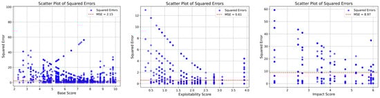
Figure 6.
Proposed model CVSS base score mean squared error plot.
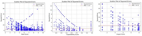
Figure 7.
Comparative model RoBERTa CVSS base score mean squared error plot.
The results in Table 6 confirm the proposed model’s superior performance across both vulnerability text datasets. These gains stem from its integrated architecture, combining clustering feature analysis, Transformer mechanisms, and TextCNN modules. By effectively fusing bidirectional encoding and token masking, the model enhances positional awareness. The Transformer’s self-attention captures global dependencies, while TextCNN extracts local patterns, collectively strengthening generalization. This optimized design yields state-of-the-art results in vulnerability severity assessment.
In CVSS, vulnerabilities with base scores in [7, 10] are judged as high-risk vulnerabilities. The model proposed has a low square error in judging the severity level of high-risk vulnerabilities, and the prediction effect is excellent, as shown in Figure 8. This shows that the model proposed can achieve a good assessment effect on high-risk vulnerabilities without any manual intervention, significantly improving the speed and accuracy of security detection.
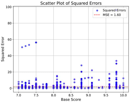
Figure 8.
Proposed model high-risk vulnerability squared error.
4.5.2. Fitted Density Plot
In this paper, we plot the real year density fitting curve and the predicted year CVSS scores density fitting curve to label vulnerability severity levels and compare the differences. Based on the density fitting graph of the experimental data, we observe that the predicted curve shows general consistency with the real curve, following the same trend. The fluctuations in the predicted curve maintain good synchronization with those in the real curve, and the error range remains within acceptable limits. Experimental results demonstrate that our model not only reasonably simulates past data distributions but also effectively predicts future trends. As Figure 9 showcases, this outcome proves the accuracy and stability of our model in capturing data patterns and verifies its generalization ability.
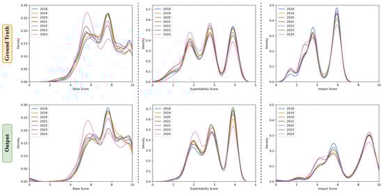
Figure 9.
Proposed model vulnerability severity assessment fitted density plot.
4.5.3. Ablation Study
To validate the impact of token masking, bidirectional encoding, clustering feature weights, and the TextCNN module on model classification performance, we constructed four model variants for ablation studies: w/o-BPE (model without bidirectional encoding), w/o-M (model without token masking), w/o-Cluster (model without cluster bias), and w/o-BPE&Mask (model lacking both bidirectional encoding and token masking modules).
As shown in Table 8, the primary performance improvement stems from the combined effect of bidirectional encoding and token-masking modules. This integrated approach enables the multi-scale fusion of word-order positioning and vulnerability features, achieving highly precise vulnerability severity classification through collaborative decision-making mechanisms.
Table 8.
Results of ablation studies.
5. Conclusions
In this paper, we present LSNet, an adaptive and efficient model that addresses suboptimal and inefficient prediction in vulnerability severity assessment. To uncover latent space features from vulnerability description texts, we design clustering algorithms and explicitly incorporate textual structural information into the self-attention mechanism of the Transformer-TextCNN architecture through bidirectional information encoding. Text features are comprehensively extracted by decomposing vector strings into labels via masked language modeling, which implicitly embeds them into the model. Extensive experiments demonstrate that LSNet effectively addresses traditional methods’ limitations: inaccurate assessments resulting from rigid vulnerability evaluation rules and inefficiencies caused by manual severity judgments.
Our method successfully extracts and integrates latent textual features to enhance assessment accuracy. However, this paper reveals certain limitations in the temporal modeling of vulnerability evolutionary characteristics. In this paper, we report considerable limitations in capturing and representing temporal dynamics inherent to the evolution of software vulnerabilities. Specifically, we encountered several challenges in modeling evolutionary patterns of vulnerability over time: On the one hand, the scarcity of consistently documented historical data across different software versions and platforms impedes the construction of continuous temporal sequences. On the other hand, the heterogeneous and non-uniform nature of vulnerability disclosures leads to fragmented and irregular time-series characteristics, complicating the learning of long-range dependencies. We utilize sophisticated data processing techniques and distinctive predictive approaches to decompose the comprehensive task of vulnerability severity assessment into manageable sub-problems, address them sequentially, and, ultimately, yield the final outcomes.
In future work, we will explore incorporating temporal analysis modules and integrating vulnerability lifecycle data to further optimize the timeliness and adaptability of severity assessments. We plan to extend the current framework by incorporating temporal analysis modules and integrating comprehensive vulnerability lifecycle data. These enhancements will allow the model to dynamically capture time-sensitive patterns and contextual shifts in threat landscapes.
Author Contributions
Methodology, Y.W.; Software, Y.W.; Formal analysis, Y.W.; Resources, J.Z.; Data curation, Y.W.; Writing—original draft, Y.W.; Writing—review & editing, J.Z. and M.H.; Funding acquisition, M.H. All authors have read and agreed to the published version of the manuscript.
Funding
This paper was supported by the National Natural Science Foundation of China with grant number 62402063, and was supported by the Natural Science Foundation of Hunan Province with grant number 2024JJ6067.
Data Availability Statement
The CCF OSC2024 dataset underlying this article is available in [competition-vd/data_1] at https://www.gitlink.org.cn/Eshe/competition-vd/dataset (accessed on 27 July 2025). The raw data NVD dataset was derived from sources in the public domain: https://nvd.nist.gov/vuln/data-feeds (accessed on 27 July 2025).
Conflicts of Interest
The authors declare no conflict of interest.
References
- IBM Annual Report 2024. 2025. Available online: https://www.ibm.com/investor/services/annual-report (accessed on 27 July 2025).
- Pan, S.; Bao, L.; Zhou, J.; Hu, X.; Xia, X.; Li, S. Towards More Practical Automation of Vulnerability Assessment. In Proceedings of the IEEE/ACM 46th International Conference on Software Engineering, Lisbon, Portugal, 14–20 April 2024. [Google Scholar]
- Spring, J.; Hatleback, E.; Householder, A.; Manion, A.; Shick, D. Time to Change the CVSS? IEEE Secur. Priv. 2021, 19, 74–78. [Google Scholar] [CrossRef]
- Gao, Z.; Yao, Y.; Yao, F.; Liu, Y.Z.; Luo, P. Predicting Model of Vulnerabilities Based on the Type of Vulnerability Severity. Acta Electrinica Sin. 2013, 41, 1784–1787. [Google Scholar]
- Zhang, P.; Xie, X. Vulnerability classification based on binary tree with entropy multi-class support vector machine. J. Comput. Appl. 2014, 34, 3283–3286. [Google Scholar]
- Zheng, J.; Kai, S.; Shi, F. Vulnerability exploitability assessment method based on network environment. J. Univ. Chin. Acad. Sci. 2024, 41, 842–852. [Google Scholar]
- Javadi, S.; Hashemy, S.; Mohammadi, K.; Howard, K.; Neshat, A. Classification of aquifer vulnerability using K-means cluster analysis. J. Hydrol. 2017, 549, 27–37. [Google Scholar] [CrossRef]
- Younis, A.A.; Yashwant, K.M. Comparing and Evaluating CVSS Base Metrics and Microsoft Rating System. In Proceedings of the 2015 IEEE International Conference on Software Quality, Reliability and Security, Washington, DC, USA, 3–5 August 2015; IEEE: New York, NY, USA, 2015. [Google Scholar]
- Naik, N.; Grace, P.; Jenkins, P.; Naik, K.; Song, J. An evaluation of potential attack surfaces based on attack tree modelling and risk matrix applied to self-sovereign identity. Comput. Secur. 2022, 120, 102808. [Google Scholar] [CrossRef]
- Qu, L.; Jia, Y.; Hao, Y. Automatic Classification of Vulnerabilities Based on CNN and Text Semantics. Transcations Beijing Inst. Technol. 2019, 39, 738–742. [Google Scholar]
- Alshubaily, I. TextCNN with attention for text classification. arXiv 2021, arXiv:2108.01921. [Google Scholar] [CrossRef]
- Sahin, C.B. DCW-RNN: Improving Class Level Metrics for Software Vulnerability Detection Using Artificial Immune System with Clock-Work Recurrent Neural Network. In Proceedings of the 2021 International Conference on INnovations in Intelligent SysTems and Applications (INISTA), Kocaeli, Turkey, 25–27 August 2021; IEEE: New York, NY, USA, 2021. [Google Scholar]
- Le, T.H.M.; Chen, H.; Babar, M.A. A survey on data-driven software vulnerability assessment and prioritization. arXiv 2021, arXiv:2107.08364. [Google Scholar] [CrossRef]
- Wu, T.; Chen, L.; Du, G.; Zhu, C.; Cui, N.; Shi, G. CDNM: Clustering-Based Data Normalization Method For Automated Vulnerability Detection. Comput. J. 2024, 67, 1538–1549. [Google Scholar] [CrossRef]
- Hao, J.; Luo, S.; Pan, L. A novel vulnerability severity assessment method for source code based on a graph neural network. Inf. Softw. Technol. 2023, 161, 107247. [Google Scholar] [CrossRef]
- Common Vulnerability Scoring System (CVSS). 2025. Available online: https://www.first.org/cvss/ (accessed on 27 July 2025).
- CVSS Vulnerability Metrics. 2025. Available online: https://nvd.nist.gov/vuln-metrics/cvss (accessed on 27 July 2025).
- Ramesh, M.; Selvan, M.T.; Sreenivas, P.; Sahayaraj, A.F. Advanced machine learning-driven characterization of new natural cellulosic Lablab purpureus fibers through PCA and K-means clustering techniques. Int. J. Biol. Macromol. 2025, 306, 141589. [Google Scholar] [CrossRef]
- Vardakas, G.; Likas, A. Global k-means++: An effective relaxation of the global k-means clustering algorithm. Appl. Intell. 2024, 54, 8876–8888. [Google Scholar] [CrossRef]
- Blackhurst, J.; Rungtusanatham, M.J.; Scheibe, K.; Ambulkar, S. Supply chain vulnerability assessment: A network based visualization and clustering analysis approach. J. Purch. Supply Manag. 2018, 24, 21–30. [Google Scholar] [CrossRef]
- Vaswani, A.; Shazeer, N.; Parmar, N.; Uszkoreit, J.; Jones, L.; Gomez, A.N.; Kaiser, Ł.; Polosukhin, I. Attention is all you need. In Proceedings of the 31st Conference on Neural Information Processing Systems (NIPS 2017), Long Beach, CA, USA, 4–9 December 2017. [Google Scholar]
- Crawshaw, M. Multi-task learning with deep neural networks: A survey. arXiv 2020, arXiv:2009.09796. [Google Scholar] [CrossRef]
- Yang, J.; Xiang, L.; Chu, P.; Wang, X.; Zhou, C. Certified Distributional Robustness on Smoothed Classifiers. IEEE Trans. Dependable Secur. Comput. 2023, 21, 876–888. [Google Scholar] [CrossRef]
- Fu, M.; Tantithamthavorn, C.K.; Nguyen, V.; Le, T. Chatgpt for Vulnerability Detection, Classification, and Repair: How Far are We? In Proceedings of the 2023 30th Asia-Pacific Software Engineering Conference (APSEC), Seoul, Republic of Korea, 4–7 December 2023; IEEE: New York, NY, USA, 2023. [Google Scholar]
- Devlin, J.; Chang, M.-W.; Lee, K.; Toutanova, K. BERT: Pre-Training of Deep Bidirectional Transformers for Language Understanding. In Proceedings of the 17th Conference of the North American Chapter of the Association for Computational Linguistics: Human Language Technologies (HLT-NAACL), Minneapolis, MN, USA, 2–7 June 2019; pp. 4171–4186. [Google Scholar]
- Kim, Y. Convolutional Neural Networks for Sentence Classification. In Proceedings of the Conference on Empirical Methods in Natural Language Processing, Doha, Qatar, 25–29 October 2014. [Google Scholar]
- Festa, D.; Novellino, A.; Hussain, E.; Bateson, L.; Casagli, N.; Confuorto, P.; Del Soldato, M.; Raspini, F. Unsupervised detection of InSAR time series patterns based on PCA and K-means clustering. Int. J. Appl. Earth Obs. Geoinf. 2023, 118, 103276. [Google Scholar] [CrossRef]
- Elbaz; Clément; Rilling, L.; Morin, C. Automated Keyword Extraction from “One-day” Vulnerabilities at Disclosure. In Proceedings of the NOMS 2020-2020 IEEE/IFIP Network Operations and Management Symposium, Budapest, Hungary, 20–24 April 2020; IEEE: New York, NY, USA, 2020. [Google Scholar]
- Kisi, O.; Heddam, S.; Parmar, K.S.; Petroselli, A.; Külls, C.; Zounemat-Kermani, M. Integration of Gaussian process regression and K means clustering for enhanced short term rainfall runoff modeling. Sci. Rep. 2025, 15, 7444. [Google Scholar] [CrossRef] [PubMed]
- Frei, M.; Kwon, J.; Tabaeiaghdaei, S.; Wyss, M.; Lenzen, C.; Perrig, A. G-sinc: Global Synchronization Infrastructure for Network Clocks. In Proceedings of the 2022 41st International Symposium on Reliable Distributed Systems (SRDS), Vienna, Austria, 19–22 September 2022; IEEE: New York, NY, USA, 2022. [Google Scholar]
- Zhu, R.; Huang, Y. Efficient and Precise Secure Generalized Edit Distance and Beyond. IEEE Trans. Dependable Secur. Comput. 2020, 19, 579–590. [Google Scholar]
- Vicarte, J.R.S.; Flanders, M.; Paccagnella, R.; Garrett-Grossman, G.; Morrison, A.; Fletche, C.W. Augury: Using Data Memory-Dependent Prefetchers to Leak Data at rest. In Proceedings of the 2022 IEEE Symposium on Security and Privacy (SP), San Francisco, CA, USA, 22–26 May 2022; IEEE: New York, NY, USA, 2022. [Google Scholar]
- Feuerriegel, S.; Maarouf, A.; Bär, D.; Geissler, D.; Schweisthal, J.; Pröllochs, N.; Robertson, C.E.; Rathje, S.; Hartmann, J.; Mohammad, S.M.; et al. Using natural language processing to analyse text data in behavioural science. Nat. Rev. Psychol. 2025, 4, 96–111. [Google Scholar] [CrossRef]
- Xu, X.; Xu, Z.; Ling, Z.; Jind, Z.; Du, S.; Pachori, R.B.; Chen, L. Comprehensive Implementation of TextCNN for Enhanced Collaboration Between Natural Language Processing and System Recommendation. In Proceedings of the International Conference on Image, Signal Processing, and Pattern Recognition (ISPP 2024), Guangzhou, China, 13 June 2024; SPIE: Bellingham, WA, USA, 2024; Volume 13180. [Google Scholar]
- Huang, T.; Xu, Z.; Yu, P.; Yi, J.; Xu, X. A Hybrid Transformer Model for Fake News Detection: Leveraging Bayesian Optimization and Bidirectional Recurrent Unit. arXiv 2025, arXiv:2502.09097. [Google Scholar]
- Le, T.H.M.; Hin, D.; Croft, R.; Babar, M.A. Deepcva: Automated Commit-Level Vulnerability Assessment with Deep Multi-Task learning. In Proceedings of the 2021 36th IEEE/ACM International Conference on Automated Software Engineering (ASE), Melbourne, Australia, 15–19 November 2021; IEEE: New York, NY, USA, 2021. [Google Scholar]
- Gardazi, N.M.; Daud, A.; Malik, M.K.; Bukhari, A.; Alsahfi, T.; Alshemaimri, B. BERT applications in natural language processing: A review. Artif. Intell. Rev. 2025, 58, 166. [Google Scholar] [CrossRef]
- Zheng, W.; Zhu, X.; Wen, G.; Zhu, Y.; Yu, H.; Gan, J. Unsupervised feature selection by self-paced learning regularization. Pattern Recognit. Lett. 2020, 132, 4–11. [Google Scholar] [CrossRef]
- Farmer; Leopold; Rosales, V.; Anderton, O.; Salvatore, A.; Braithwaite, R. Optimizing human-controlled preference alignment in large language models via dense token masking: A methodological approach. Authorea, 14 October 2024. [Google Scholar]
- Pang, H.; Li, C. A BERT and TextCNN Integration-Based Method for Public Complaints and Proposals Text Classification. In Proceedings of the 8th International Conference on Computer Science and Application Engineering, Shanghai, China, 28–29 November 2024. [Google Scholar]
- He, P.; Liu, X.; Gao, J.; Chen, W. Deberta: Decoding-enhanced bert with disentangled attention. arXiv 2020, arXiv:2006.03654. [Google Scholar]
- Lan, Z. Albert: A lite bert for self-supervised learning of language representations. arXiv 2019, arXiv:1909.11942. [Google Scholar]
- Liu, Y. Roberta: A robustly optimized bert pretraining approach. arXiv 2019, arXiv:1907.11692. [Google Scholar]
Disclaimer/Publisher’s Note: The statements, opinions and data contained in all publications are solely those of the individual author(s) and contributor(s) and not of MDPI and/or the editor(s). MDPI and/or the editor(s) disclaim responsibility for any injury to people or property resulting from any ideas, methods, instructions or products referred to in the content. |
© 2025 by the authors. Licensee MDPI, Basel, Switzerland. This article is an open access article distributed under the terms and conditions of the Creative Commons Attribution (CC BY) license (https://creativecommons.org/licenses/by/4.0/).