A Novel q-Type Semi-Dependent Neutrosophic Decision-Making Approach and Its Applications in Supplier Selection

Abstract

The principles of least effort and the illusion of control may influence the decision-making process. It is challenging for a decision-maker to maintain complete independence when assessing the membership and non-membership degrees of indicators. However, existing neutrosophic sets and q-rung orthopair fuzzy sets assume full independence of such information. In view of this, this paper proposes a new neutrosophic set, namely the q-type semi-dependent neutrosophic set (QTSDNS), based on the classical neutrosophic set, whose membership and non-membership degrees are interrelated. QTSDNS is a generalized form of classical semi-dependent fuzzy sets, such as the intuitionistic neutrosophic set. It contains a regulatory parameter, which allows for decision-makers to flexibly adjust the model. Furthermore, a multi-attribute group decision-making (MAGDM) algorithm is proposed by integrating QTSDNS with evidence theory to solve the supplier selection problem. The algorithm first utilizes QTSDNS to represent the preference information of experts, then employs the q-TSDNWAA (or q-TSDNWGA) operator to aggregate the evaluation information of individual experts. Following the analysis of the mathematical relationship between QTSDNS and evidence theory, evidence theory is used to aggregate the evidence from each expert to obtain the group trust interval. Then, the best supplier is determined using interval number ranking methods. Finally, a numerical example is provided to demonstrate the feasibility of the proposed method.

1. Introduction

Under the backdrop of global economic integration, globally diversified procurement helps enterprises to quickly, flexibly, and efficiently meet the needs of downstream customers at a lower cost. Procurement strategies can be categorized into single-source and multi-source procurement based on the number of suppliers. Multi-source procurement reduces dependency on individual suppliers, mitigates supply risks, and fosters competition among suppliers to secure better pricing and services. For example, industries such as power generation, automotive parts, agricultural commodities, electronic components, and other highly standardized products typically adopt multi-source procurement strategies. It is essential for enterprises to select suppliers scientifically. In earlier research, supplier evaluation primarily focused on economic performance. With the emergence and evolution of the concept of sustainable development, the supplier evaluation system has gradually incorporated a comprehensive set of indicators, including economic, environmental, and social performance. However, due to the limitations of individual decision-makers’ knowledge and expertise, it is difficult to conduct a comprehensive and balanced assessment when dealing with such complex decision-making problems. This necessitates collaboration among multiple decision-makers to combine their collective wisdom.

Therefore, multi-attribute group decision-making (MAGDM) is one of the main approaches for addressing supplier selection problems. Whether the evaluation value of indicators can accurately express the preferences of decision experts is a key factor in determining the accuracy of decision models. Fuzzy set theory is an efficient information modeling tool with high information richness and flexibility, widely used in different decision-making fields, such as security risk assessment [1], charging station location selection [2], infectious disease hospital location selection [3], project investment risk assessment [4], new energy vehicle battery recycling [5], supplier selection [6], enterprise selection of cost-effective production plans [7], dengue fever prevention and control strategy selection [8], and medical service quality evaluation during epidemics [9].

Smarandache proposed Neutrosophic Set (NS) [10], which has been widely studied over the past few decades [11,12,13,14]. For the convenience of information modeling, Wang further proposed the single-valued neutrosophic set (SVNS), which consists of truth membership function (TMF), indeterminacy membership function (IMF), and falsity membership function (FMF) [15]. The constraint conditions for SVNS are $0\le TMF+IMF+FMF\le 3$. However, in NS and SVNS, TMF, IMF, and FMF are assumed to be mutually independent. In 2016, Smarandache further discussed the NS, where TMF, IMF, and FMF have interdependent relationships [16]. The semi-dependent NS has attracted the attention of many scholars. Monoranjan and Madhumangal provided the intuitionistic neutrosophic set (INS) in the case where TMF and FMF are dependent intuitionistic fuzzy (IF) numbers, and $0\le TMF+IMF+FMF\le 2$ [17]. Jansi et al. provided the Pythagorean neutrosophic set (PNS) under the condition where TMF and FMF are interdependent Pythagorean fuzzy (PF) numbers, and $0\le TM{F}^2+IM{F}^2+$$FM{F}^2\le 2$ [18]. PNS has significantly expanded the application scope of semi-dependent NS, but it still falls short of being sufficiently broad. For example, when a decision-making expert evaluates a certain attribute, they consider the TMF and FMF to be 50% dependent on each other, with the values of the TMF, IMF, and FMF being 0.7, 0.8, and 0.8, respectively. Despite $0\le {0.7}^2+{0.8}^2+{0.8}^2\le 2$, since ${0.7}^2+{0.8}^2=1.13>1$, the condition that TMF and FMF are dependent in a Pythagorean fuzzy relationship is therefore not satisfied. Drawing on the information modeling method of q-rung orthopair fuzzy sets, which enhances the model’s capability by increasing the value of the exponent. As shown in Figure 1, the information modeling capability is significantly enhanced as q increases. For example, if the exponent is 3, $0\le {0.7}^3+$${0.8}^3+{0.8}^3\le 2$, ${0.7}^3+$${0.7}^3+{0.8}^3=$$0.86<1$. This indicates that TMF and FMF exhibit a three-rung orthopair fuzzy dependence.

To evaluate big data capabilities in manufacturing supply chains, Feng et al. developed a MAGDM model based on Pythagorean fuzzy sets [19]. Choudhary et al. proposed an intuitionistic fuzzy supply chain evaluation model from the perspective of sustainable development capacity [20]. Pamucar et al. defined neutrosophic information aggregation operators under Dombi norms and applied them to solve multi-attribute decision-making problems for supplier selection [21]. Priyadharshini et al. investigated the green supplier selection problem under a complex neutrosophic fuzzy environment and proposed a MAGDM method based on Schweizer–Sklar operators [22]. Riaz et al. utilized q-rung orthopair fuzzy sets to represent supplier evaluation information and developed a MAGDM method with prioritized aggregation operators, which was applied to baby crib supplier selection [23]. All the above studies assume that the membership degree, non-membership degree, and other indicators of evaluation information are independent of each other. However, in complex fuzzy environments, decision-makers’ cognitive and emotional biases often make it difficult to provide completely independent assessment information. Furthermore, evidence theory is an effective tool for handling uncertainty and conflict in information, yet it has been rarely used in existing group decision-making models, especially in the context of supply chain management problems.

The motivation of this study stems from enhancing the information modeling capability of existing semi-dependent fuzzy sets and enriching the theoretical framework for group decision-making in supplier selection problems. The main contributions of this paper are as follows:

• Proposes a broader semi-dependent fuzzy set QTSDNS, which is the general form of PNS, INS, IF set, PF set, q-type orthopair fuzzy set, and so on;
• Operational rules and information fusion operators for q-type semi-dependent neutrosophic numbers have been developed, facilitating the application of QTSDNS in practical decision-making models with semi-dependent characteristics;
• An evidence-based information fusion method for q-type semi-dependent neutrosophic numbers is proposed;
• A q-type semi-dependent group decision-making algorithm was proposed based on evidence theory and the developed operators. This method was applied to solve a supplier selection problem in the intelligent vehicle industry, thereby extending the scope of research on fuzzy supplier selection. The decision-making method proposed in this paper has a wide range of application scenarios and can be extended to decision-making fields such as human resource recruitment, investment project selection, green building scheme selection, and medical scheme selection.

The remainder of this paper is structured as follows: In Section 2, we review evidence theory and introduce the concept and operational rules of QTSDNS. In Section 3, a q-TSDNWAA operator and a q-TSDNWGA operator are developed. In Section 4, a group decision-making algorithm is proposed, combining the evidence information fusion method for q-type semi-dependent neutrosophic numbers and the q-TSDNWAA (or q-TSDNWGA) operator. In Section 5 and Section 6, through a simulation experiment involving the selection of radar and laser display suppliers for intelligent automobiles, the effectiveness of the algorithm presented in this article is demonstrated, and the impact of parameters on the group decision-making model is analyzed. A comparative study is conducted in Section 7. Finally, in Section 8, a summary and outlook are provided for the research work on q-type semi-dependent neutrosophic numbers conducted in this article.

2. Preliminaries

In this section, we will review and present some important theories that will facilitate further research in this paper.

2.1. Evidence Theory

In decision-making methods based on evidence theory [24,25], the decision-maker’s preferences are represented by a mass function. The mass function can reasonably describe “incomplete information”, “imprecise information”, and “uncertain information”. The mass function is built on the basis of an identification framework. Therefore, we first need to clarify the concept of the identification framework. Suppose there is a judgment problem, and let $F$ represent the complete set of all possible answers to this judgment problem. If all elements in the complete set $F$ are mutually independent, then this set of mutually exclusive events is called the identification framework. The Belief measure (Bel) and Plausibility measure (Pl) are defined as

$$Bel(A)={\displaystyle \sum _{B\subseteq A}m(B)}, PI(A)={\displaystyle \sum _{B\cap A\ne \varnothing }m(B)},$$

where $A\subset F,B\subset F$, $m:2^F\to [0,1]$, $m(\varnothing )=0$, ${\displaystyle \sum _{A\in F}m(A)}=1$, and $m$ is the basic probability assignment (BPA) function.

Next, we introduce another important concept in evidence theory: the evidence combination function.

Definition 1

([26]). Let $m_1,m_2,\dots ,m_n$ be a collection of BPA functions under the same identification framework $F$, with the corresponding pieces of evidence $A_1,A_2,\dots ,$ $A_n$, then

$$m(A)=m_1(A_1)\oplus m_2(A_2)\oplus \dots m_n(A_n)=\left\{\begin{array}{ll}0,& A=\varnothing .\\ {\displaystyle \frac{{\displaystyle \sum _{A_1\cap A_2\cap \dots \cap A_n=A}{m}_1(A_1)m_2(A_2)\dots m_n(A_n)}}{1-{\displaystyle \sum _{A_1\cap A_2\cap \dots \cap A_n=\varnothing }{m}_1(A_1)m_2(A_2)\dots m_n(A_n)}}},& A\ne \varnothing .\end{array}\right.$$

2.2. Fuzzy Sets

Definition 2

([15]). A single-valued neutrosophic set (SVNS) $\aleph$ defined on the finite set $\Im$ is given with $\aleph =\{<x,T_{\aleph }(x),I_{\aleph }(x),F_{\aleph }(x)>,x\in \Im \}$, where $T_{\aleph }(x)$, $I_{\aleph }(x)$ and $F_{\aleph }(x)$ are the TMF, IMF and FMF. $\forall x\in \Im$, $0\le T_{\aleph }(x)\le 1$, $0\le I_{\aleph }(x)\le 1$, $0\le F_{\aleph }(x)\le 1$ and $0\le T_{\aleph }(x)+I_{\aleph }(x)+F_{\aleph }(x)\le 3$

However, in actual decision-making, the TMF, IMF, and FMF provided by evaluators are often not entirely independent; especially, the TMF and FMF tend to be interdependent. Given this, scholars have proposed the semi-dependent fuzzy set.

Definition 3

([17]). An intuitionistic neutrosophic set (INS) $\aleph$ defined on the finite set $\Im$ is given with ${\aleph }^{\#}=\{<x,T_{{\aleph }^{\#}}(x),I_{{\aleph }^{\#}}(x),F_{{\aleph }^{\#}}(x)>,x\in \Im \}$, where $T_{{\aleph }^{\#}}(x)$, $I_{{\aleph }^{\#}}(x)$ and $F_{{\aleph }^{\#}}(x)$ are the TMF, IMF and FMF. $\forall x\in \Im$, $0\le T_{{\aleph }^{\#}}(x)\le 1$, $0\le I_{{\aleph }^{\#}}(x)\le 1$, $0\le F_{{\aleph }^{\#}}(x)\le 1$ and $0\le T_{\aleph }(x)+I_{\aleph }(x)+F_{\aleph }(x)\le 2$. $T_{{\aleph }^{\#}}(x)$ and $F_{{\aleph }^{\#}}(x)$ have a dependent intuitionistic fuzzy relationship, whereas $I_{{\aleph }^{\#}}(x)$ is an independent function.

Definition 4

([18]). A Pythagorean neutrosophic set (PNS) ${\aleph }^{†}$ defined on the finite set $\Im$ is given with ${\aleph }^{†}=\{<x,T_{{\aleph }^{†}}(x),I_{{\aleph }^{†}}(x),F_{{\aleph }^{†}}(x)>,x\in \Im \}$, where $T_{{\aleph }^{†}}(x)$, $I_{{\aleph }^{†}}(x)$ and $F_{{\aleph }^{†}}(x)$ are the TMF, IMF and FMF. $\forall x\in \Im$, $0\le T_{{\aleph }^{†}}(x)\le 1$, $0\le I_{{\aleph }^{†}}(x)\le 1$, $0\le F_{{\aleph }^{†}}(x)\le 1$ and $0\le T_{{\aleph }^{†}}^2(x)+I_{{\aleph }^{†}}^2(x)+F_{{\aleph }^{†}}^2(x)\le 2$. $T_{{\aleph }^{†}}(x)$ and $F_{{\aleph }^{†}}(x)$ have a dependent Pythagorean fuzzy relationship, whereas $I_{{\aleph }^{†}}(x)$ is an independent function.

Based on the research of semi-dependent fuzzy set, we define a q-type semi-dependent neutrosophic set (QTSDNS).

Definition 5.

A QTSDNS $\Xi$ defined on the finite set $\Im$ is given with $\Xi =\{<x,T_{\Xi }(x),I_{\Xi }(x),F_{\Xi }(x)>,x\in \Im \}$, where $T_{\Xi }(x)$, $I_{\Xi }(x)$ and $F_{\Xi }(x)$ are the TMF, IMF and FMF. $\forall x\in \Im$, $q>0$, $0\le T_{\Xi }(x)\le 1$, $0\le I_{\Xi }(x)\le 1$, $0\le F_{\Xi }(x)\le 1$ and $0\le T_{\Xi }^q(x)+I_{\Xi }^q(x)+F_{\Xi }^q(x)\le 2$, $T_{\Xi }(x)$ and $F_{\Xi }(x)$ have a q-rung orthopair fuzzy dependent relationship, whereas $I_{\Xi }(x)$ is an independent function. Convenience, a q-type semi-dependent neutrosophic number (QTSDNN) is denoted by $\mathbf{\gamma }=<T,I,F>$

Remark 

(1)

If $T_{\Xi }(x)=0$, then QTSDNS degrades to q-rung orthopair fuzzy set [23];

(2)

If $T_{\Xi }(x)=0$ and $q=2$, then QTSDNS degrades to Pythagorean fuzzy set [19];

(3)

If $T_{\Xi }(x)=0$ and $q=1$, then QTSDNS degrades to intuitionistic fuzzy set [20];

(4)

If $T_{\Xi }(x)=0$ and $I_{\Xi }(x)=0$, then QTSDNS degrades to q-type fuzzy set [23];

(5)

If $T_{\Xi }(x)=0$, $I_{\Xi }(x)=0$ and $q=1$, then QTSDNS degrades to fuzzy set [5];

(6)

If $q=1$, then QTSDNS degrades to intuitionistic neutrosophic set [17];

(7)

If $q=2$, then QTSDNS degrades to Pythagorean neutrosophic set [18].

As can be seen from

Table 1. Comparative analysis of different fuzzy sets.

Set	Representation Function	Constraint Condition	Whether Independent
Fuzzy set	TMF	$0\le TMF\le 1$.	YES
Intuitionistic fuzzy set	TMF, IMF	$0\le TMF,IMF\le 1;0\le TMF+IMF\le 1$.	YES
Pythagorean fuzzy set	TMF, IMF	$0\le TMF,IMF\le 1;0\le TM{F}^2+IM{F}^2\le 1$.	YES
q-rung orthopair fuzzy set	TMF, IMF	$0\le TMF,IMF\le 1;0\le TM{F}^q+IM{F}^q\le 1$.	YES
Neutrosophic set	TMF, IMF, FMF	$0\le TMF,FMF,IMF\le 1;0\le TMF+FMF+IMF\le 3$.	YES
Intuitionistic neutrosophic set	TMF, IMF, FMF	$0\le TMF,FMF,IMF\le 1;0\le TMF+FMF+IMF\le 2$.	Semi- dependent
Pythagorean neutrosophic set	TMF, IMF, FMF	$0\le TMF,FMF,IMF\le 1;0\le TM{F}^2+FM{F}^2+IM{F}^2\le 2.$	Semi- dependent
q-type semi-dependent neutrosophic set	TMF, IMF, FMF	$0\le TMF,FMF,IMF\le 1;0\le TM{F}^q+FM{F}^q+IM{F}^q\le 2.$	Semi- dependent

, compared with classical fuzzy sets such as intuitionistic fuzzy sets and Pythagorean fuzzy sets, QTSDNS employs three functions (TMF, IMF, and FMF) to represent decision-making information in a richer and more comprehensive manner. Similar to intuitionistic neutrosophic sets and Pythagorean neutrosophic sets, QTSDNS discusses information modeling under conditions related to TMF and FMF, thereby enriching the theoretical framework of fuzzy information. Furthermore, as analyzed in the Remark section, QTSDNS is a more generalized form of semi-dependent fuzzy sets.

Definition 6.

Let $\phi =<T,I,F>$ is a QTSDNN, then $S(\phi )={\displaystyle \frac{2+T-I-F}{3}}$ is the score of $\phi$. IF $\gamma =<T_1,I_1,F_1>$ and $\phi =<T_2,I_2,F_2>$ be two QTSDNNs, then (1) if $S(\gamma )>S(\phi )$, then $\gamma >\phi$; (2) if $S(\gamma )=S(\phi )$, then $\gamma =\phi$

Here, we provide some operational rules involving QTSDNN.

Definition 7.

Let $\gamma =<T_1,I_1,F_1>$ and $\phi =<T_2,I_2,F_2>$ be any two QTSDNNs and $\lambda >0$, then

(1)

$\gamma \oplus \phi =〈{(T_1^q+T_2^q-T_1^q{T}_2^q)}^{1/q},I_1{I}_2,F_1{F}_2〉$;

(2)

$\gamma \otimes \phi =〈T_1{T}_2,{(I_1^q+I_2^q-I_1^q{I}_2^q)}^{1/q},{(F_1^q+F_2^q-F_1^q{F}_2^q)}^{1/q}〉$;

(3)

$\lambda \gamma =〈{(1-{(1-T_1^q)}^{\lambda })}^{1/q},I_1^{\lambda },F_1^{\lambda }〉$;

(4)

${\gamma }^{\lambda }=〈T_1^{\lambda },{(1-{(1-I_1^q)}^{\lambda })}^{1/q},{(1-{(1-F_1^q)}^{\lambda })}^{1/q}〉$.

Theorem 1.

Let $\gamma =<T_1,I_1,F_1>$ and $\phi =<T_2,I_2,F_2>$ be any two QTSDNNs and $l>0$, $l_1>0$ and $l_2>0$, then (1) $\gamma \oplus \phi =\phi \oplus \gamma$; (2) $\gamma \otimes \phi =\phi \otimes \gamma$; (3) $l(\gamma \oplus \phi )=l\phi \oplus l\gamma$; (4) $l_1\gamma \oplus l_2\gamma =(l_1+l_2)\gamma$; (5) ${\gamma }^{l_1}\otimes {\gamma }^{l_2}={\gamma }^{l_1+l_2}$; (6) ${\gamma }^l\otimes {\phi }^l={(\phi \otimes \gamma )}^l$

Proof. 

(1) $\gamma \oplus \phi =〈{(T_1^q+T_2^q-T_1^q{T}_2^q)}^{1/q},I_1{I}_2,F_1{F}_2〉$ $=\phi \oplus \gamma$.

(2) $\gamma \otimes \phi =〈T_1{T}_2,{(I_1^q+I_2^q-I_1^q{I}_2^q)}^{1/q},{(F_1^q+F_2^q-F_1^q{F}_2^q)}^{1/q}〉=\phi \otimes \gamma$.

(3) $l(\gamma \oplus \phi )=l〈{(T_1^q+T_2^q-T_1^q{T}_2^q)}^{1/q},I_1{I}_2,F_1{F}_2〉$

$=〈{\left(1-{(1-T_1^q-T_2^q+T_1^q{T}_2^q)}^l\right)}^{1/q},I_1^l{I}_2^l,F_1^l{F}_2^l〉$.

$l\phi \oplus l\gamma$ $=〈{(1-{(1-T_1^q)}^l)}^{1/q},I_1^l,F_1^l〉\oplus 〈{(1-{(1-T_2^q)}^l)}^{1/q},I_2^l,F_2^l〉$

$=〈{\left(1-{(1-T_1^q)}^l+1-{(1-T_2^q)}^l-(1-{(1-T_1^q)}^l)(1-{(1-T_2^q)}^l)\right)}^{1/q},I_1^l{I}_2^l,F_1^l{F}_2^l〉$

$=〈{\left(1-{(1-T_1^q-T_2^q+T_1^q{T}_2^q)}^l\right)}^{1/q},I_1^l{I}_2^l,F_1^l{F}_2^l〉=l(\gamma \oplus \phi )$.

(4) $l_1\gamma \oplus l_2\gamma =〈{(1-{(1-T_1^q)}^{l_1})}^{1/q},I_1^{l_1},F_1^{l_1}〉\oplus 〈{(1-{(1-T_1^q)}^{l_2})}^{1/q},I_1^{l_2},F_1^{l_2}〉$

$=〈{\left(1-{(1-T_1^q)}^{l_1}+1-{(1-T_1^q)}^{l_2}+(1-{(1-T_1^q)}^{l_1})(1-{(1-T_1^q)}^{l_2})\right)}^{1/q},I_1^{l_1}\cdot I_1^{l_2},F_1^{l_1}\cdot F_1^{l_2}〉$

$=〈{(1-{(1-T_1^q)}^{l_1+l_2})}^{1/q},I_1^{l_1+l_2},F_1^{l_1+l_2}〉=(l_1+l_2)\gamma .$

(5) ${\gamma }^{l_1}\otimes {\gamma }^{l_2}$

$=〈T_1^{l_1},{(1-{(1-I_1^q)}^{l_1})}^{1/q},{(1-{(1-F_1^q)}^{l_1})}^{1/q}〉\otimes 〈T_1^{l_2},{(1-{(1-I_1^q)}^{l_2})}^{1/q},{(1-{(1-F_1^q)}^{l_2})}^{1/q}〉$

$=〈T_1^{l_1}{T}_1^{l_2},{\left(1-{(1-I_1^q)}^{l_1}{(1-I_1^q)}^{l_2}\right)}^{1/q},$ ${\left(1-{(1-F_1^q)}^{l_1}{(1-F_1^q)}^{l_2}\right)}^{1/q}〉$

$=〈T_1^{l_1+l_2},{\left(1-{(1-I_1^q)}^{l_1+l_2}\right)}^{1/q},$ ${\left(1-{(1-F_1^q)}^{l_1+l_2}\right)}^{1/q}〉$ $={\gamma }^{l_2+l_2}$.

(6) ${\gamma }^l\otimes {\phi }^l$ $=〈T_1^l,{(1-{(1-I_1^q)}^l)}^{1/q},{(1-{(1-F_1^q)}^l)}^{1/q}〉\otimes 〈T_2^l,{(1-{(1-I_2^q)}^l)}^{1/q},{(1-{(1-F_2^q)}^l)}^{1/q}〉$ $=〈T_1^l{T}_2^l,{\left(1-{(1-I_1^q)}^l+1-{(1-I_2^q)}^l+(1-{(1-I_1^q)}^l)(1-{(1-I_2^q)}^l)\right)}^{1/q},$ ${\left(1-{(1-F_1^q)}^l+1-{(1-F_2^q)}^l+(1-{(1-F_1^q)}^l)(1-{(1-F_2^q)}^l)\right)}^{1/q}〉$

$=〈T_1^l{T}_2^l,{(1-{(1-I_1^q)}^l{(1-I_2^q)}^l)}^{1/q},{(1-{(1-F_1^q)}^l{(1-F_2^q)}^l)}^{1/q}〉$.

${(\gamma \otimes \phi )}^l={〈T_1{T}_2,{(I_1^q+I_2^q-I_1^q{I}_2^q)}^{1/q},{(F_1^q+F_2^q-F_1^q{F}_2^q)}^{1/q}〉}^l$

$=〈{(T_1{T}_2)}^l,{(1-{(1-I_1^q-I_2^q+I_1^q{I}_2^q)}^l)}^{1/q},{(1-{(1-F_1^q-F_2^q+F_1^q{F}_2^q)}^l)}^{1/q}〉$

$=〈T_1^l{T}_2^l,{(1-{(1-I_1^q)}^l{(1-I_2^q)}^l)}^{1/q},{(1-{(1-F_1^q)}^l{(1-F_2^q)}^l)}^{1/q}〉$

$={(\gamma \otimes \phi )}^l$. □

3. Aggregation Operators for QTSDNNs

Here, we will define and discuss the semi-dependent operators.

Definition 8.

Let ${\gamma }_i=<T_i,I_i,F_i>,i=1,\dots ,n$ be a collection of QTSDNNs with the weight $w_i\ge 0,i=1,\dots ,n,{\displaystyle \sum _{i=1}^n{w}_i}=1$. Then, the q-TSDNWAA operator is defined as q-TSDNWAA $({\gamma }_1,{\gamma }_2,\dots ,{\gamma }_n)=(w_1{\gamma }_1)\oplus (w_2{\gamma }_2)\oplus \dots \oplus (w_n{\gamma }_n)$.

Theorem 2.

Let ${\gamma }_i=<T_i,I_i,F_i>,i=1,\dots ,n$ be a collection of QTSDNNs with the weight $w_i\ge 0,i=1,\dots ,n,{\displaystyle \sum _{i=1}^n{w}_i}=1$. Then

$$\mathrm{q}-\mathrm{TSDNWAA}({\gamma }_1,{\gamma }_2,\dots ,{\gamma }_n)=〈{(1-\prod _{i=1}^n{(1-T_i^q)}^{w_i})}^{1/q},\prod _{i=1}^n{I}_i^{w_i},\prod _{i=1}^n{F}_i^{w_i}〉.$$

(1)

Proof. 

For $n=2$, then we get

q-TSDNWAA $({\gamma }_1,{\gamma }_2)=(w_1{\gamma }_1)\oplus (w_2{\gamma }_2)$

$=〈{(1-{(1-T_1^q)}^{w_1})}^{1/q},I_1^{w_1},F_1^{w_1}〉\oplus 〈{(1-{(1-T_2^q)}^{w_2})}^{1/q},I_2^{w_2},F_2^{w_2}〉$

$=〈{\left(1-{(1-T_1^q)}^{w_1}+1-{(1-T_2^q)}^{w_2}-(1-{(1-T_1^q)}^{w_1})(1-{(1-T_2^q)}^{w_2})\right)}^{1/q},I_1^{w_1}{I}_2^{w_2},F_1^{w_1}{F}_2^{w_2}〉$ $=〈{(1-\prod _{i=1}^2{(1-T_i^q)}^{w_i})}^{1/q},\prod _{i=1}^2{I}_i^{w_i},\prod _{i=1}^2{F}_i^{w_i}〉$. □

When $n=k$, $k\ge 2$ suppose that

$$\mathrm{q}-\mathrm{TSDNWAA}({\gamma }_1,{\gamma }_2,\dots ,{\gamma }_k)=〈{(1-\prod _{i=1}^k{(1-T_i^q)}^{w_i})}^{1/q},\prod _{i=1}^k{I}_i^{w_i},\prod _{i=1}^k{F}_i^{w_i}〉.$$

Then $n=k+1$, we have,

q-TSDNWAA $({\gamma }_1,{\gamma }_2,\dots ,{\gamma }_k,{\gamma }_{k+1})$

$=〈{(1-{\displaystyle \prod _{i=1}^k}{(1-T_i^q)}^{w_i})}^{1/q},{\displaystyle \prod _{i=1}^k}{I}_i^{w_i},{\displaystyle \prod _{i=1}^k}{F}_i^{w_i}〉\oplus 〈{(1-{(1-T_{k+1}^q)}^{w_{k+1}})}^{1/q},I_{k+1}^{w_{k+1}},F_{k+1}^{w_{k+1}}〉$

$\begin{array}{l}=\langle {\left(1-{\displaystyle \prod _{i=1}^k}{(1-T_i^q)}^{w_i}+1-{(1-T_{k+1}^q)}^{w_{k+1}}-(1-{\displaystyle \prod _{i=1}^k}{(1-T_i^q)}^{w_i})(1-{(1-T_{k+1}^q)}^{w_{k+1}})\right)}^{1/q},\\ {\displaystyle \prod _{i=1}^k}{I}_i^{w_i}\times I_{k+1}^{w_{k+1}},{\displaystyle \prod _{i=1}^k}{F}_i^{w_i}\times F_{k+1}^{w_{k+1}}\rangle \end{array}$

$=〈{(1-{\displaystyle \prod _{i=1}^{k+1}}{(1-T_i^q)}^{w_i})}^{1/q},{\displaystyle \prod _{i=1}^{k+1}}{I}_i^{w_i},\prod _{i=1}^{k+1}{F}_i^{w_i}〉$.

So, Equation (1) is true for all n.

Theorem 3

(Idempotency). Let  ${\gamma }_i=<T_i,I_i,F_i>,i=1,\dots ,n$ be a collection of QTSDNNs with the weight $w_i\ge 0,i=1,\dots ,n,{\displaystyle \sum _{i=1}^n{w}_i}=1$. If${\gamma }_i=<T_0,I_0,F_0>,i=1,\dots ,n$

$$\mathrm{Then} \mathrm{q}-\mathrm{TSDNWAA}({\gamma }_1,{\gamma }_2,\dots ,{\gamma }_n)=<T_0,I_0,F_0>.$$

(2)

Proof. 

q-TSDNWAA $({\gamma }_1,{\gamma }_2,\dots ,{\gamma }_n)=〈{(1-{\displaystyle \prod _{i=1}^n}{(1-T_i^q)}^{w_i})}^{1/q},{\displaystyle \prod _{i=1}^n}{I}_i^{w_i},{\displaystyle \prod _{i=1}^n}{F}_i^{w_i}〉$

$=〈{(1-{\displaystyle \prod _{i=1}^n}{(1-T_0^q)}^{w_i})}^{1/q},{\displaystyle \prod _{i=1}^n}{I}_0^{w_i},{\displaystyle \prod _{i=1}^n}{F}_0^{w_i}〉$$=〈{(1-{\displaystyle \prod _{i=1}^n}{(1-T_0^q)}^{w_i})}^{1/q},{\displaystyle \prod _{i=1}^n}{I}_0^{w_i},{\displaystyle \prod _{i=1}^n}{F}_0^{w_i}〉$

$=〈{(1-{(1-T_0^q)}^{{\displaystyle \sum _{i=1}^n{w}_i}})}^{1/q},I_0^{{\displaystyle \sum _{i=1}^n{w}_i}},F_0^{{\displaystyle \sum _{i=1}^n{w}_i}}〉=〈{(1-(1-T_0^q))}^{1/q},I_0,F_0〉=<T_0,I_0,F_0>$. □

Theorem 4

(Idempotency). Let ${\gamma }_i=<T_i,I_i,F_i>,{\gamma }^{\prime }i=<T^{\prime }i,I^{\prime }i,F^{\prime }i>,i=1,\dots ,n$ be two collection of QTSDNNs with the same weight $w_i\ge 0,i=1,\dots ,n,{\displaystyle \sum _{i=1}^n{w}_i}=1$. If $T_i\ge T_i^{\prime },$ $I_i\le I_i^{\prime },$ $F_i\le F_i^{\prime },$ $i=1,\dots ,n$, then

$$\mathrm{q}-\mathrm{TSDNWAA}({\gamma }_1,{\gamma }_2,\dots ,{\gamma }_n)\ge \mathrm{q}-\mathrm{TSDNWAA}({\gamma }_1^{\prime },{\gamma }_2^{\prime },\dots ,{\gamma }_n^{\prime })$$

(3)

Proof. 

For any i, $T_i\ge T_i^{\prime },I_i\le I_i^{\prime },$ $F_i\le F_i^{\prime }.$ Hence, ${\displaystyle {\displaystyle \prod }_{i=1}^n}{I}_i\le {\displaystyle {\displaystyle \prod }_{i=1}^n}{I}_i^{\prime },{\displaystyle {\displaystyle \prod }_{i=1}^n}{F}_i\le {\displaystyle {\displaystyle \prod }_{i=1}^n}{F}_i^{\prime }$.

and

$T_i^q\ge T_i^{\prime q}\Rightarrow 1-T_i^q\le 1-T_i^{\prime q}\Rightarrow {(1-T_i^q)}^{w_i}\le {(1-T_i^{\prime q})}^{w_i}\Rightarrow {\displaystyle {\displaystyle \prod }_{i=1}^n}{(1-T_i^q)}^{w_i}\le {\displaystyle {\displaystyle \prod }_{i=1}^n}{(1-T_i^{\prime q})}^{w_i}$.

$\Rightarrow 1-{\displaystyle {\displaystyle \prod }_{i=1}^n}{(1-T_i^q)}^{w_i}\ge 1-{\displaystyle {\displaystyle \prod }_{i=1}^n}{(1-T_i^{\prime q})}^{w_i}$.

$\Rightarrow {\displaystyle \frac{2+(1-{\displaystyle {\displaystyle \prod }_{i=1}^n}{(1-T_i^q)}^{w_i})-{\displaystyle {\displaystyle \prod }_{i=1}^n}{I}_i-{\displaystyle {\displaystyle \prod }_{i=1}^n}{F}_i}{3}}\ge {\displaystyle \frac{2+(1-{\displaystyle {\displaystyle \prod }_{i=1}^n}{(1-T_i^{\prime q})}^{w_i})-{\displaystyle {\displaystyle \prod }_{i=1}^n}{I}_i^{\prime }-{\displaystyle {\displaystyle \prod }_{i=1}^n}{F}_i^{\prime }}{3}}$.

$\Rightarrow$q-TSDNWAA $({\gamma }_1,{\gamma }_2,\dots ,{\gamma }_k)=〈{(1-{\displaystyle \prod _{i=1}^k}{(1-T_i^q)}^{w_i})}^{1/q},{\displaystyle \prod _{i=1}^k}{I}_i^{w_i},{\displaystyle \prod _{i=1}^k}{F}_i^{w_i}〉$.

$\ge 〈{(1-{\displaystyle \prod _{i=1}^k}{(1-{T^{\prime }}_i^q)}^{w_i})}^{1/q},{\displaystyle \prod _{i=1}^k}{I^{\prime }}_i^{w_i},{\displaystyle \prod _{i=1}^k}{F^{\prime }}_i^{w_i}〉=$q-TSDNWAA $({\gamma }^{\prime }1,{\gamma }^{\prime }2,\dots ,{\gamma }^{\prime }n)$.

Theorem 5

(Boundedness). Let ${\gamma }_i=<T_i,I_i,F_i>,i=1,\dots ,n$ be a collection of QTSDNNs with the weigh t $w_i\ge 0,i=1,\dots ,n,{\displaystyle \sum _{i=1}^n{w}_i}=1$. If ${\gamma }^{-}=<\underset{1\le k\le n}{\min }{T}_k,\underset{1\le k\le n}{\max }{I}_k,\underset{1\le k\le n}{\max }{F}_k>$ and ${\gamma }^{+}=<\underset{1\le k\le n}{\max }{T}_k,\underset{1\le k\le n}{\min }{I}_k,\underset{1\le k\le n}{\min }{F}_k>$ then

$${\gamma }^{-}\le \mathrm{q}-\mathrm{TSDNWAA}({\gamma }_1,{\gamma }_2,\dots ,{\gamma }_n)\le {\gamma }^{+}.$$

(4)

Proof. 

Since ${(1-\underset{1\le k\le n}{\max }{T}_k^q)}^{w_i}\le {(1-T_k^q)}^{w_i}\le {(1-\underset{1\le k\le n}{\min }{T}_k^q)}^{w_i}.$

$\Rightarrow {\displaystyle {\displaystyle \prod }_{i=1}^n}{(1-\underset{1\le k\le n}{\max }{T}_k^q)}^{w_i}\le {\displaystyle {\displaystyle \prod }_{i=1}^n}{(1-T_i^q)}^{w_i}\le {\displaystyle {\displaystyle \prod }_{i=1}^n}{(1-\underset{1\le k\le n}{\min }{T}_k^q)}^{w_i}$.

$\Rightarrow 1-\underset{1\le k\le n}{\max }{T}_k^q\le {\displaystyle {\displaystyle \prod }_{i=1}^n}{(1-T_i^q)}^{w_i}\le 1-\underset{1\le k\le n}{\min }{T}_k^q$.

$\Rightarrow {\displaystyle \frac{2+\underset{1\le k\le n}{\min }{T}_k^q-\underset{1\le k\le n}{\max }{I}_k-\underset{1\le k\le n}{\max }{F}_k}{3}}\le {\displaystyle \frac{2+(1-{\displaystyle {\displaystyle \prod }_{i=1}^n}{(1-T_i^q)}^{w_i})-{\displaystyle {\displaystyle \prod }_{i=1}^n}{I}_i^{w_i}-{\displaystyle {\displaystyle \prod }_{i=1}^n}{F}_i^{w_i}}{3}}\le {\displaystyle \frac{2+\underset{1\le k\le n}{\max }{T}_k^q-\underset{1\le k\le n}{\min }{I}_k-\underset{1\le k\le n}{\min }{F}_k}{3}}$.

$\Rightarrow <\underset{1\le k\le n}{\min }{T}_k,\underset{1\le k\le n}{\max }{I}_k,\underset{1\le k\le n}{\max }{F}_k>\le 〈{(1-{\displaystyle \prod _{i=1}^k}{(1-T_i^q)}^{w_i})}^{1/q},{\displaystyle \prod _{i=1}^k}{I}_i^{w_i},{\displaystyle \prod _{i=1}^k}{F}_i^{w_i}〉\le <\underset{1\le k\le n}{\max }{T}_k,\underset{1\le k\le n}{\min }{I}_k,\underset{1\le k\le n}{\min }{F}_k>$.

$\Rightarrow {\gamma }^{-}\le$q-TSDNWAA $({\gamma }_1,{\gamma }_2,\dots ,{\gamma }_n)\le {\gamma }^{+}$. □

Definition 9.

Let  ${\gamma }_i=<T_i,I_i,F_i>,i=1,\dots ,n$ be a collection of QTSDNNs with the weight $w_i\ge 0,i=1,\dots ,n,{\displaystyle \sum _{i=1}^n{w}_i}=1$. Then, the q-TSDNWGA operator is defined as

$$\mathrm{q}-\mathrm{TSDNWGA}({\gamma }_1,{\gamma }_2,\dots ,{\gamma }_n)=({\gamma }_1{w}_1)\otimes ({\gamma }_2{w}_2)\otimes \dots \otimes ({\gamma }_n{w}_n).$$

Theorem 6.

Let ${\gamma }_i=<T_i,I_i,F_i>,i=1,\dots ,n$ be a collection of QTSDNNs with the weight $w_i\ge 0,i=1,\dots ,n,{\displaystyle \sum _{i=1}^n{w}_i}=1$. Then

$$\mathrm{q}-\mathrm{TSDNWGA}({\gamma }_1,{\gamma }_2,\dots ,{\gamma }_n)=〈\prod _{i=1}^n{T}_i^{w_i},{(1-\prod _{i=1}^n{(1-I_i^q)}^{w_i})}^{1/q},{(1-\prod _{i=1}^n{(1-F_i^q)}^{w_i})}^{1/q}〉.$$

(5)

Proof. 

For $n=2$, then we get

q-TSDNWGA $({\gamma }_1,{\gamma }_2)={\gamma }_1{w}_1\otimes {\gamma }_2{w}_2$

$=〈T_1^{w_1},{(1-{(1-I_1^q)}^{w_1})}^{1/q},{(1-{(1-F_1^q)}^{w_1})}^{1/q}〉\otimes 〈T_2^{w_2},{(1-{(1-I_2^q)}^{w_2})}^{1/q},{(1-{(1-F_2^q)}^{w_2})}^{1/q}〉$

$=〈T_1^{w_1}{T}_2^{w_2},{\left(1-{(1-I_1^q)}^{w_1}+1-{(1-I_2^q)}^{w_2}-(1-{(1-I_1^q)}^{w_1})(1-{(1-I_2^q)}^{w_2})\right)}^{1/q},$

${\left(1-{(1-F_1^q)}^{w_1}+1-{(1-F_2^q)}^{w_2}-(1-{(1-F_1^q)}^{w_1})(1-{(1-F_2^q)}^{w_2})\right)}^{1/q}〉$

$=〈T_1^{w_1}{T}_2^{w_2},{\left(1-{(1-I_1^q)}^{w_1}{(1-I_2^q)}^{w_2}\right)}^{1/q},{\left(1-{(1-F_1^q)}^{w_1}{(1-F_2^q)}^{w_2}\right)}^{1/q}〉$$=〈{\displaystyle \prod _{i=1}^2}{T}_i^{w_i},{(1-{\displaystyle \prod _{i=1}^2}{(1-I_i^q)}^{w_i})}^{1/q},{(1-{\displaystyle \prod _{i=1}^2}{(1-F_i^q)}^{w_i})}^{1/q}〉$. □

When $n=k$, $k\ge 2$ suppose that

$$\mathrm{q}-\mathrm{TSDNWGA}({\gamma }_1,{\gamma }_2,\dots ,{\gamma }_k)=〈\prod _{i=1}^k{T}_i^{w_i},{(1-\prod _{i=1}^k{(1-I_i^q)}^{w_i})}^{1/q},{(1-\prod _{i=1}^k{(1-F_i^q)}^{w_i})}^{1/q}〉.$$

Then $n=k+1$, we have,

$$\mathrm{q}-\mathrm{TSDNWGA}({\gamma }_1,{\gamma }_2,\dots ,{\gamma }_k,{\gamma }_{k+1})$$

$$=〈\prod _{i=1}^k{T}_i^{w_i},{(1-\prod _{i=1}^k{(1-I_i^q)}^{w_i})}^{1/q},{(1-\prod _{i=1}^k{(1-F_i^q)}^{w_i})}^{1/q}〉\oplus 〈T_{k+1}^{w_{k+1}},{(1-{(1-I_{k+1}^q)}^{w_{k+1}})}^{1/q},{(1-{(1-F_{k+1}^q)}^{w_{k+1}})}^{1/q}〉$$

$$=〈\prod _{i=1}^k{T}_i^{w_i}\times T_{k+1}^{w_{k+1}},{\left(1-\prod _{i=1}^k{(1-I_i^q)}^{w_i}+1-{(1-I_{k+1}^q)}^{w_{k+1}}-(1-\prod _{i=1}^k{(1-I_i^q)}^{w_i})(1-{(1-I_{k+1}^q)}^{w_{k+1}})\right)}^{1/q},$$

$${\left(1-\prod _{i=1}^k{(1-F_i^q)}^{w_i}+1-{(1-F_{k+1}^q)}^{w_{k+1}}-(1-\prod _{i=1}^k{(1-F_i^q)}^{w_i})(1-{(1-F_{k+1}^q)}^{w_{k+1}})\right)}^{1/q}〉$$

$$=〈\prod _{i=1}^{k+1}{T}_i^{w_i},{(1-\prod _{i=1}^{k+1}{(1-I_i^q)}^{w_i})}^{1/q},{(1-\prod _{i=1}^{k+1}{(1-F_i^q)}^{w_i})}^{1/q}〉.$$

So, Equation (5) is true for all n.

Theorem 7

(Idempotency). Let ${\gamma }_i=<T_i,I_i,F_i>,i=1,\dots ,n$ be a collection of QTSDNNs with the weight $w_i\ge 0,i=1,\dots ,n,{\displaystyle \sum _{i=1}^n{w}_i}=1$. If ${\gamma }_i=<T_0,I_0,F_0>,i=1,\dots ,n$, then

$$\mathrm{q}-\mathrm{TSDNWGA}({\gamma }_1,{\gamma }_2,\dots ,{\gamma }_n)=<T_0,I_0,F_0>.$$

(6)

Proof. 

q-TSDNWGA $({\gamma }_1,{\gamma }_2,\dots ,{\gamma }_n)=〈{\displaystyle \prod _{i=1}^n}{T}_i^{w_i},{(1-{\displaystyle \prod _{i=1}^n}{(1-I_i^q)}^{w_i})}^{1/q},{(1-{\displaystyle \prod _{i=1}^n}{(1-F_i^q)}^{w_i})}^{1/q}〉$

$=〈{\displaystyle \prod _{i=1}^n}{T}_0^{w_i},{(1-{\displaystyle \prod _{i=1}^n}{(1-I_0^q)}^{w_i})}^{1/q},{(1-{\displaystyle \prod _{i=1}^n}{(1-F_0^q)}^{w_i})}^{1/q}〉$

$=〈{\displaystyle \prod _{i=1}^n}{T}_0^{w_i},{(1-{\displaystyle \prod _{i=1}^n}{(1-I_0^q)}^{w_i})}^{1/q},{(1-{\displaystyle \prod _{i=1}^n}{(1-F_0^q)}^{w_i})}^{1/q}〉$

$=〈T_0^{{\displaystyle \sum _{i=1}^n{w}_i}},{(1-{(1-I_0^q)}^{{\displaystyle \sum _{i=1}^n{w}_i}})}^{1/q},{(1-{(1-F_0^q)}^{{\displaystyle \sum _{i=1}^n{w}_i}})}^{1/q}〉$

$=〈T_0,{(1-(1-I_0^q))}^{1/q},{(1-(1-F_0^q))}^{1/q}〉=<T_0,I_0,F_0>$. □

Theorem 8

(Idempotency). Let ${\gamma }_i=<T_i,I_i,F_i>,{\gamma }^{\prime }i=<T^{\prime }i,I^{\prime }i,F^{\prime }i>,i=1,\dots ,n$ be two collection of QTSDNNs with the same weight $w_i\ge 0,i=1,\dots ,n,{\displaystyle \sum _{i=1}^n{w}_i}=1$. If $T_i\ge T_i^{\prime },$ $I_i\le I_i^{\prime },$ $F_i\le F_i^{\prime },$ $i=1,\dots ,n$, then

$$\mathrm{q}-\mathrm{TSDNWGA}({\gamma }_1,{\gamma }_2,\dots ,{\gamma }_n)\ge \mathrm{q}-\mathrm{TSDNWGA}({\gamma }_1^{\prime },{\gamma }_2^{\prime },\dots ,{\gamma }_n^{\prime }).$$

(7)

Proof. 

For any i, $T_i\ge T_i^{\prime },I_i\le I_i^{\prime },$$F_i\le F_i^{\prime }.$ Hence, ${\displaystyle {\displaystyle \prod }_{i=1}^n}{T}_i\ge {\displaystyle {\displaystyle \prod }_{i=1}^n}{T}_i^{\prime }$ and

$1-I_i^q\ge 1-I_i^{\prime q},1-F_i^q\ge 1-F_i^{\prime q}$. $\Rightarrow {(1-I_i^q)}^{w_i}\ge {(1-I_i^{\prime q})}^{w_i},{(1-F_i^q)}^{w_i}\ge {(1-F_i^{\prime q})}^{w_i}$.

$\Rightarrow {\displaystyle {\displaystyle \prod }_{i=1}^n}{(1-I_i^q)}^{w_i}\ge {\displaystyle {\displaystyle \prod }_{i=1}^n}{(1-I_i^{\prime q})}^{w_i},{\displaystyle {\displaystyle \prod }_{i=1}^n}{(1-F_i^q)}^{w_i}\ge {\displaystyle {\displaystyle \prod }_{i=1}^n}{(1-F_i^{\prime q})}^{w_i}$.

$\Rightarrow 1-{\displaystyle {\displaystyle \prod }_{i=1}^n}{(1-I_i^q)}^{w_i}\le 1-{\displaystyle {\displaystyle \prod }_{i=1}^n}{(1-I_i^{\prime q})}^{w_i},1-{\displaystyle {\displaystyle \prod }_{i=1}^n}{(1-F_i^q)}^{w_i}\le 1-{\displaystyle {\displaystyle \prod }_{i=1}^n}{(1-F_i^{\prime q})}^{w_i}$.

$\Rightarrow {\displaystyle \frac{2+{\displaystyle \prod _{i=1}^n}{T}_i^{w_i}-{(1-{\displaystyle \prod _{i=1}^n}{(1-I_i^q)}^{w_i})}^{1/q}-{(1-{\displaystyle \prod _{i=1}^n}{(1-F_i^q)}^{w_i})}^{1/q}}{3}}\ge$  ${\displaystyle \frac{2+{\displaystyle \prod _{i=1}^n}{T^{\prime }}_i^{w_i}-{(1-{\displaystyle \prod _{i=1}^n}{(1-{I^{\prime }}_i^q)}^{w_i})}^{1/q}-{(1-{\displaystyle \prod _{i=1}^n}{(1-{F^{\prime }}_i^q)}^{w_i})}^{{1/q}_{\prime }^i}}{3}}$.

$\Rightarrow$q-TSDNWGA $({\gamma }_1,{\gamma }_2,\dots ,{\gamma }_n)=〈{\displaystyle \prod _{i=1}^n}{T}_i^{w_i},{(1-{\displaystyle \prod _{i=1}^n}{(1-I_i^q)}^{w_i})}^{1/q},{(1-{\displaystyle \prod _{i=1}^n}{(1-F_i^q)}^{w_i})}^{1/q}〉$

$\ge 〈{\displaystyle \prod _{i=1}^n}{T^{\prime }}_i^{w_i},{(1-{\displaystyle \prod _{i=1}^n}{(1-{I^{\prime }}_i^q)}^{w_i})}^{1/q},{(1-{\displaystyle \prod _{i=1}^n}{(1-{F^{\prime }}_i^q)}^{w_i})}^{1/q}〉=$q-TSDNWGA $({\gamma }^{\prime }1,{\gamma }^{\prime }2,\dots ,{\gamma }^{\prime }n)$. □

Theorem 9

(Boundedness). Let ${\gamma }_i=<T_i,I_i,F_i>,i=1,\dots ,n$ be a collection of QTSDNNs with the weight $w_i\ge 0,i=1,\dots ,n,{\displaystyle \sum _{i=1}^n{w}_i}=1$. If ${\gamma }^{-}=<\underset{1\le k\le n}{\min }{T}_k,\underset{1\le k\le n}{\max }{I}_k,\underset{1\le k\le n}{\max }{F}_k>$

$$\mathrm{and} {\gamma }^{+}=<\underset{1\le k\le n}{\max }{T}_k,\underset{1\le k\le n}{\min }{I}_k,\underset{1\le k\le n}{\min }{F}_k>, \mathrm{then} {\gamma }^{-}\le q-\mathrm{TSDNWGA}({\gamma }_1,{\gamma }_2,\dots ,{\gamma }_n)\le {\gamma }^{+}.$$

(8)

Proof. 

Since ${(1-\underset{1\le k\le n}{\max }{I}_k^q)}^{w_i}\le {(1-I_i^q)}^{w_i}\le {(1-\underset{1\le k\le n}{\min }{I}_k^q)}^{w_i}$, ${(1-\underset{1\le k\le n}{\max }{I}_k^q)}^{w_i}\le$${(1-I_i^q)}^{w_i}\le$${(1-\underset{1\le k\le n}{\min }{I}_k^q)}^{w_i}$$\Rightarrow {\displaystyle \prod }_{i=1}^n{(1-\underset{1\le k\le n}{\max }{I}_k^q)}^{w_i}\le {\displaystyle \prod }_{i=1}^n{(1-I_k^q)}^{w_i}\le {\displaystyle \prod }_{i=1}^n{(1-\underset{1\le k\le n}{\min }{I}_k^q)}^{w_i}$,

and

$${\displaystyle \prod }_{i=1}^n{(1-\underset{1\le k\le n}{\max }{F}_k^q)}^{w_i}\le {\displaystyle \prod }_{i=1}^n{(1-F_i^q)}^{w_i}\le {\displaystyle \prod }_{i=1}^n{(1-\underset{1\le k\le n}{\min }{F}_k^q)}^{w_i}.$$

$$\Rightarrow 1-\underset{1\le k\le n}{\max }{I}_k^q\le \prod _{i=1}^n{(1-I_i^q)}^{w_i}\le 1-\underset{1\le k\le n}{\min }{I}_k^q,1-\underset{1\le k\le n}{\max }{F}_k^q\le \prod _{i=1}^n{(1-F_i^q)}^{w_i}\le 1-\underset{1\le k\le n}{\min }{F}_k^q.$$

$$\begin{gathered} \Rightarrow {\displaystyle \frac{2+\underset{1\le k\le n}{\min }{T}_k^q-\underset{1\le k\le n}{\max }{I}_k-\underset{1\le k\le n}{\max }{F}_k}{3}}\le {\displaystyle \frac{2+\prod _{i=1}^k{T}_i^{w_i}-{(1-\prod _{i=1}^k{(1-I_i^q)}^{w_i})}^{1/q}-{(1-\prod _{i=1}^k{(1-F_i^q)}^{w_i})}^{1/q}}{3}}\le {\displaystyle \frac{2+\underset{1\le k\le n}{\max }{T}_k^q-\underset{1\le k\le n}{\min }{I}_k-\underset{1\le k\le n}{\min }{F}_k}{3}} \\ \Rightarrow <\underset{1\le k\le n}{\min }{T}_k,\underset{1\le k\le n}{\max }{I}_k,\underset{1\le k\le n}{\max }{F}_k>\le 〈\prod _{i=1}^k{T}_i^{w_i},{(1-\prod _{i=1}^k{(1-I_i^q)}^{w_i})}^{1/q},{(1-\prod _{i=1}^k{(1-F_i^q)}^{w_i})}^{1/q}〉\le <\underset{1\le k\le n}{\max }{T}_k,\underset{1\le k\le n}{\min }{I}_k,\underset{1\le k\le n}{\min }{F}_k> \end{gathered}$$

$\Rightarrow {\gamma }^{-}\le$ q-TSDNWGA $({\gamma }_1,{\gamma }_2,\dots ,{\gamma }_n)\le {\gamma }^{+}$. □

Example 1.

Assume that  ${\gamma }_1=(0.4,0.5,0.3)$,${\gamma }_2=(0.3,0.4,0.2)$,${\gamma }_3=(0.6,0.3,0.3)$ are three QTSDNNs with the weight vector of $w=(0.4,0.25,0.35)$. The following aggregation is performed using the q-TSDNWAA and q-TSDNWGA operators, respectively. Using the q-TSDNWAA operator (here, q = 2), the calculation process is as follows.

$$\begin{array}{c} \mathrm{q}-\mathrm{TSDNWAA}({\gamma }_1,{\gamma }_2,{\gamma }_3)\hfill \\ =〈{(1-{(1-{0.4}^2)}^{0.4}\times {(1-{0.3}^2)}^{0.25}\times {(1-{0.6}^2)}^{0.35})}^{1/2},{0.5}^{0.4}\times {0.4}^{0.25}\times {0.3}^{0.35},{0.3}^{0.4}\times {0.2}^{0.25}\times {0.3}^{0.35}〉\hfill \\ =〈0.459,0.395,0.271〉.\hfill \end{array}$$

Using the q-TSDNWGA operator (here, q = 2), the calculation process is as follows.

$$\begin{gathered} \mathrm{q}-\mathrm{TSDNWGA}({\gamma }_1,{\gamma }_2,{\gamma }_3) \\ =〈{0.4}^{0.4}\times {0.3}^{0.25}\times {0.6}^{0.35},{(1-{(1-{0.5}^2)}^{0.4}\times {(1-{0.4}^2)}^{0.25}\times {(1-{0.3}^2)}^{0.35})}^{1/2},{0.3}^{0.4}\times {0.2}^{0.25}\times {0.3}^{0.35}〉 \\ =〈0.429,0.411,0.276〉 \end{gathered}$$

As shown in Figure 2, under identical parameters, the aggregated value score derived from the q-TSDNWAA operator significantly differs from that of the q-TSDNWGA operator. Specifically, the q-TSDNWAA operator yields a higher score than the q-TSDNWGA operator. Consequently, during aggregation, optimistic decision-makers may prefer the q-TSDNWAA operator, whereas pessimistic ones may opt for the q-TSDNWGA operator. This divergence stems from their fundamental construction principles: The q-TSDNWAA operator employs an arithmetic mean-based approach, demonstrating strong compensability (where high values in one attribute can offset low values in others). The q-TSDNWGA operator utilizes a geometric mean-based approach, emphasizing synergistic effects among attributes.

4. MAGDM Using QTSDNN

In this section, we will combine evidence theory with the operators proposed earlier (q-TSDNWAA operator and q-TSDNWGA operator) to present a decision framework for q-type semi-dependent neutrosophic MAGDM problems.

Let $X=(x_1,x_2,$$\dots ,x_n\}$ be a set of alternatives, $C=(c_1,c_2,$$\dots ,c_m\}$ be the attributes, and $w={(w_1,w_2,\dots ,w_n)}^T$ be the weights of alternatives, ${\displaystyle \sum _{i=1}^n{w}_i}=1$, $w_i\in [0,1]$, and $D=(d_1,d_2,$$\dots ,d_r\}$ be a set of experts. ${\gamma }_{ij}^k=<T_{ij}^k,I_{ij}^k,F_{ij}^k>,$ $i=1,$ $\dots ,n;j=1,\dots ,m;k=1,\dots ,r$, where ${\gamma }_{ij}^k$ denotes the QTSDNN of $x_i$ under $c_j$ provided by expert $d_k$. The q-type semi-dependent neutrosophic decision matrix ${\gamma }^{(k)}$ by expert $d_k$ is defined as

$${\gamma }^{(k)}=\left(\begin{array}{cccc}{\gamma }_{11}^k& {\gamma }_{12}^k& \dots & {\gamma }_{1m}^k\\ {\gamma }_{21}^k& {\gamma }_{22}^k& \dots & {\gamma }_{2m}^k\\ ⋮& ⋮& ⋮& ⋮\\ {\gamma }_{n1}^k& {\gamma }_{n2}^k& \dots & {\gamma }_{nm}^k\end{array}\right).$$

Step 1. Transform the q-type semi-dependent neutrosophic decision matrix ${\gamma }^{(k)}$ into a normalized matrix ${\gamma }^{(k)\prime }={\left({\gamma }_{ij}^{(k)\prime }\right)}_{n\times m}$, where

$${\gamma }_{ij}^{(k)\prime }=\left\{\begin{array}{ll}{\gamma }_{ij}^{(k)},& \mathrm{if} \mathrm{the} \mathrm{criteria} c_j\mathrm{is} \mathrm{benefit} \mathrm{type},\\ N({\gamma }_{ij}^{(k)})=<T_{ij}^k,1-I_{ij}^k,F_{ij}^k>,& \mathrm{if} \mathrm{the} \mathrm{criteria} c_j\mathrm{is} \cos \mathrm{t} \mathrm{type}.\end{array}\right.$$

Step 2. Integrate the kth line of ${\gamma }^{(k)\prime }={\left({\gamma }_{ij}^{(k)\prime }\right)}_{n\times m}$ by the q-TSDNWAA (or q-TSDNW-GA) operator, and get the information fusion matrix $\mathfrak{M}={({\mathfrak{M}}_{kj})}_{r\times n}={(<{\mathfrak{T}}_{kj},{\Im }_{kj},{\mathfrak{J}}_{kj}>)}_{r\times n}$ of expert $d_k$, where ${\mathfrak{M}}_{kj}=$q-TSDNWAA $(h_{j1}^{(k)},h_{j2}^{(k)},\dots ,h_{jm}^{(k)})$, $j=1,2,\dots ,n$; $k=1,2,\dots ,r$ or ${\mathfrak{M}}_{kj}=$q-TSDNWGA $(h_{j1}^{(k)},h_{j2}^{(k)},\dots ,h_{jm}^{(k)})$, $j=1,2,\dots ,n$; $k=1,2,\dots ,r$.

Step 3. Transform the information fusion matrix $\mathfrak{M}={({\mathfrak{M}}_{kj})}_{r\times n}$ into a standardized matrix ${\mathfrak{M}}^{\prime }={({{\mathfrak{M}}^{\prime }}_{kj})}_{r\times n}={(<{{\mathfrak{T}}^{\prime }}_{kj},{{\Im }^{\prime }}_{kj},{{\mathfrak{J}}^{\prime }}_{kj}>)}_{r\times n}$, where

$$<{{\mathfrak{T}}^{\prime }}_{kj},{{\Im }^{\prime }}_{kj},{{\mathfrak{J}}^{\prime }}_{kj}>=<{\displaystyle \frac{{\mathfrak{T}}_{kj}}{\underset{1\le k\le r,1\le j\le n}{\max }({\mathfrak{T}}_{kj}+{\Im }_{kj}+{\mathfrak{J}}_{kj})}},{\displaystyle \frac{{\Im }_{kj}}{\underset{1\le k\le r,1\le j\le n}{\max }({\mathfrak{T}}_{kj}+{\Im }_{kj}+{\mathfrak{J}}_{kj})}},{\displaystyle \frac{{\mathfrak{J}}_{kj}}{\underset{1\le k\le r,1\le j\le n}{\max }({\mathfrak{T}}_{kj}+{\Im }_{kj}+{\mathfrak{J}}_{kj})}}>.$$

Step 4. Based on the definition of QTSDNN, we consider the individual integrated information as evidence information. QTSDNN can be regarded as containing three types of information: the complete acceptance of the attributes of candidate solutions (accept), the complete disapproval (reject), and the hesitation between acceptance and disapproval (accept, reject). According to the Evidence theory, the complete set can be defined $F=${accept, reject}. So, the power set $F$ is $\left\{\varnothing \right.,${accept},{reject},{accept, reject $\left.\}\right\}$. The BPA can be defined $m(\varnothing )$, m({accept}), m({reject}), m({accept, reject}). F or ${{\mathfrak{M}}^{\prime }}_{kj}$, by referring to references [1,2,3], it can be considered that

$$m_{kj}\left(\mathrm{accept}\right)={{\mathfrak{T}}^{\prime }}_{kj};m_{kj}\left(\mathrm{reject}\right)={{\mathfrak{J}}^{\prime }}_{kj};m_{kj}(\mathrm{accept}, \mathrm{reject})={{\Im }^{\prime }}_{kj}$$

Using the evidence combination formula

$$M_i(A)=m_{1i}(A_1)\oplus m_{2i}(A_2)\oplus \dots \oplus m_{li}(A_l)={\displaystyle \frac{{\displaystyle \sum _{A_1\cap A_2\cap \dots \cap A_l=A}{m}_{1i}(A_1)m_{2i}(A_2)\dots m_{li}(A_l)}}{1-{\displaystyle \sum _{A_1\cap A_2\cap \dots \cap A_l=\varnothing }{m}_{1i}(A_1)m_{2i}(A_2)\dots m_{li}(A_l)}}},$$

where $A,A_1,A_2,\dots ,A_l\in \{$accept, reject, (accept, reject)}, we obtain the group evidence information $M_i=(M_i\left(\right\{\mathrm{accept}\left\}\right),M_i\left(\right\{\mathrm{accept}, \mathrm{reject}\left\}\right),M_i\left(\right\{ \mathrm{reject}\left\}\right)$ of $x_i$, $i=1,\dots ,n$.

Step 5. Based on the group evidence information $M_i$, calculate the group trust interval $I_i$ for alternatives, where $I_i=$ [Bel $(x_i)$, Pl $(x_i)$], $i=1,\dots ,n$.

Step 6. Calculate the possibility matrix $P={\left(p_{ij}\right)}_{n\times n}$, where

$$p_{ij}=\left\{\begin{array}{l}1-{\displaystyle \frac{1}{2e^{\frac{\mathrm{Pl}(x_i)-\mathrm{Bel}(x_j)}{\left[\mathrm{Pl}\right(x_i)-\mathrm{Bel}(x_i\left)\right]+\left[\mathrm{Pl}\right(x_j)-\mathrm{Bel}(x_j\left)\right]}-0.5}}},{\displaystyle \frac{\mathrm{Pl}(x_i)-\mathrm{Bel}(x_j)}{\left[\mathrm{Pl}\right(x_i)-\mathrm{Bel}(x_i\left)\right]+\left[\mathrm{Pl}\right(x_j)-\mathrm{Bel}(x_j\left)\right]}}\ge 0.5\\ {\displaystyle \frac{1}{2e^{0.5-\frac{\mathrm{Pl}(x_i)-\mathrm{Bel}(x_j)}{\left[\mathrm{Pl}\right(x_i)-\mathrm{Bel}(x_i\left)\right]+\left[\mathrm{Pl}\right(x_j)-\mathrm{Bel}(x_j\left)\right]}}}},{\displaystyle \frac{\mathrm{Pl}(x_i)-\mathrm{Bel}(x_j)}{\left[\mathrm{Pl}\right(x_i)-\mathrm{Bel}(x_i\left)\right]+\left[\mathrm{Pl}\right(x_j)-\mathrm{Bel}(x_j\left)\right]}}<0.5\end{array}\right..$$

Step 7. If $P_j=\max \left\{P_1,P_2,\dots ,P_n\right\}$, where $P_i={\displaystyle \frac{1}{n(n-1)}}({\displaystyle \sum _{j=1}^n{p}_{ij}}-1+{\displaystyle \frac{n}{2}})$, $i\in \left\{1,2,\dots ,n\right\}$ then the optimal alternative is $x_j$ [27].

Figure 3 presents the detailed workflow of the proposed methodology described in the algorithm above.

5. Illustrative Example

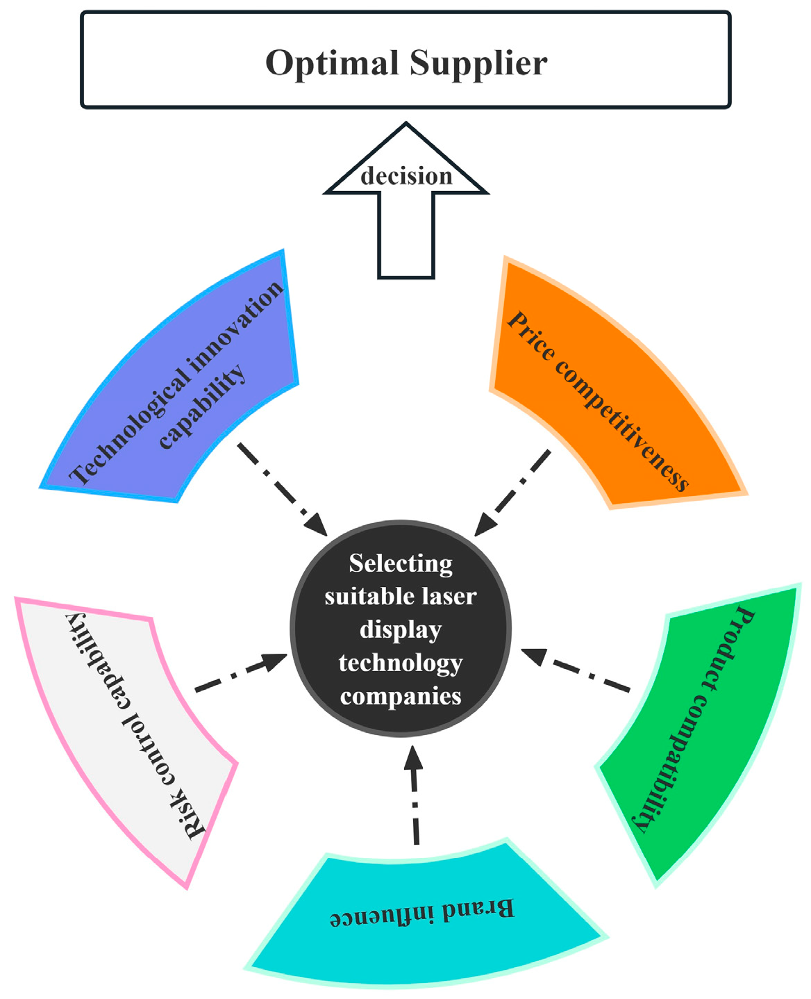
In this section, an investment appraisal project is employed to demonstrate the application of the proposed decision-making approach, as well as the validity and effectiveness of the proposed approach. The Chinese auto market, as one of the largest and most innovative strategic areas globally, is fully embracing intelligent transformation. As a key element for achieving differentiation in smart vehicles, the smart cockpit has become a highly sought-after area in the automotive industry. This trend generates new demands for in-vehicle optics and stimulates innovative applications of laser technology in this field. With the development of intelligent vehicles, there has been a notable increase in industrial cooperation, with deep collaboration between automotive companies and tech firms. Some car manufacturers prefer to choose partners with global advantages to provide smart vehicle solutions. Therefore, in the field of smart cockpits, selecting suitable laser display technology companies for collaboration will be a focus and challenge for automotive enterprises. A certain automotive company, after thorough market research and analysis, selected five technology companies {x₁, x₂, x₃, x₄, x₅} as potential partners for optimal collaboration. Given the complexity of the corporate project, three decision-making experts {e1, e2, e3} were invited to conduct a comprehensive assessment. The experts used fuzzy sets as a tool to represent evaluation information, evaluating the five technology companies across five dimensions, which are shown in Figure 4 (the weighting vector is w = (0.15, 0.25, 0.25, 0.15, 0.2)^T):

$c_1$—Price competitiveness: Supply chain cost control is an effective means for enterprises to achieve cost management, enabling them to plan and utilize various resources rationally during production and operations. Effective control of the cost prices of automotive parts directly affects the price competitiveness of the enterprise’s smart automobile products in the market.

$c_2$—Technological innovation capability: Products with technological innovation capability can increase their appeal, making consumers more eager to purchase them. In the increasingly competitive market environment, continuously advancing technological innovation and selecting components with technological innovation capability in supply chain procurement to enhance the technological content of products are of significant importance for enterprises to build new competitive advantages and promote healthy development.

$c_3$—Risk control capability: Risk management capability provides systematic assistance for enterprises to identify, evaluate, and respond to potential risks, helping them to make reasonable decisions in the face of uncertainty. Selecting suppliers with high risk-management capabilities as partners can secure sustainable partnerships, thereby providing long-term assurance for the maintenance and repair of components in the future.

$c_4$—Brand influence: Parts suppliers with strong social influence typically have a good brand image and reputation, which can help to enhance the brand image of automotive manufacturers. Furthermore, a good reputation among parts suppliers can reduce the risk of negative news, thereby protecting the brand value of smart automobile manufacturers.

$c_5$—Product compatibility: Selecting parts suppliers with compatibility is crucial for improving the production efficiency of automotive manufacturers, enhancing product quality, and maintaining market competitiveness. For example, parts with strong compatibility can simplify the design and manufacturing processes of vehicles, reducing the time and costs required for additional design or adjustments due to mismatched parts.

They provided pairwise comparisons for these companies and gave their decision information matrices in the form of QTSDNNs, as shown in

Table 2. q-type semi-dependent neutrosophic matrix ${\gamma }^{(1)}$.

	${\mathit{c}}_1$	${\mathit{c}}_2$	${\mathit{c}}_3$	${\mathit{c}}_4$	${\mathit{c}}_5$
$x_1$	$〈0.3,0.7,0.5〉$	$〈0.7,0.4,0.5〉$	$〈0.7,0.5,0.6〉$	$〈0.4,0.8,0.2〉$	$〈0.6,0.5,0.3〉$
$x_2$	$〈0.6,0.5,0.5〉$	$〈0.8,0.2,0.7〉$	$〈0.9,0.5,0.5〉$	$〈0.4,0.7,0.6〉$	$〈0.7,0.4,0.6〉$
$x_3$	$〈0.4,0.3,0.5〉$	$〈0.2,0.6,0.3〉$	$〈0.8,0.3,0.3〉$	$〈0.5,0.6,0.7〉$	$〈0.5,0.4,0.6〉$
$x_4$	$〈0.5,0.7,0.3〉$	$〈0.6,0.4,0.4〉$	$〈0.8,0.2,0.7〉$	$〈0.5,0.5,0.4〉$	$〈0.4,0.6,0.3〉$
$x_5$	$〈0.4,0.6,0.4〉$	$〈0.7,0.5,0.5〉$	$〈0.9,0.4,0.4〉$	$〈0.7,0.7,0.3〉$	$〈0.2,0.6,0.4〉$

,

Table 3. q-type semi-dependent neutrosophic matrix ${\gamma }^{(2)}$.

	${\mathit{c}}_1$	${\mathit{c}}_2$	${\mathit{c}}_3$	${\mathit{c}}_4$	${\mathit{c}}_5$
$x_1$	$〈0.4,0.8,0.6〉$	$〈0.6,0.7,0.6〉$	$〈0.4,0.9,0.5〉$	$〈0.4,0.5,0.5〉$	$〈0.4,0.7,0.5〉$
$x_2$	$〈0.7,0.4,0.4〉$	$〈0.8,0.3,0.5〉$	$〈0.7,0.2,0.2〉$	$〈0.4,0.4,0.6〉$	$〈0.4,0.6,0.8〉$
$x_3$	$〈0.4,0.5,0.2〉$	$〈0.6,0.8,0.6〉$	$〈0.6,0.7,0.6〉$	$〈0.5,0.3,0.2〉$	$〈0.5,0.4,0.6〉$
$x_4$	$〈0.5,0.7,0.5〉$	$〈0.6,0.6,0.8〉$	$〈0.5,0.3,0.8〉$	$〈0.5,0.6,0.8〉$	$〈0.5,0.8,0.2〉$
$x_5$	$〈0.3,0.6,0.6〉$	$〈0.7,0.3,0.3〉$	$〈0.7,0.5,0.5〉$	$〈0.7,0.7,0.6〉$	$〈0.7,0.7,0.4〉$

and

Table 4. q-type semi-dependent neutrosophic matrix ${\gamma }^{(3)}$.

	${\mathit{c}}_1$	${\mathit{c}}_2$	${\mathit{c}}_3$	${\mathit{c}}_4$	${\mathit{c}}_5$
$x_1$	$〈0.7,0.7,0.5〉$	$〈0.8,0.5,0.3〉$	$〈0.6,0.7,0.3〉$	$〈0.6,0.6,0.6〉$	$〈0.2,0.6,0.3〉$
$x_2$	$〈0.6,0.4,0.6〉$	$〈0.9,0.2,0.4〉$	$〈0.9,0.2,0.5〉$	$〈0.4,0.6,0.2〉$	$〈0.4,0.4,0.5〉$
$x_3$	$〈0.5,0.6,0.2〉$	$〈0.8,0.4,0.2〉$	$〈0.7,0.3,0.6〉$	$〈0.3,0.8,0.8〉$	$〈0.7,0.5,0.7〉$
$x_4$	$〈0.3,0.8,0.6〉$	$〈0.6,0.5,0.8〉$	$〈0.7,0.2,0.4〉$	$〈0.4,0.7,0.5〉$	$〈0.5,0.7,0.5〉$
$x_5$	$〈0.2,0.7,0.4〉$	$〈0.9,0.3,0.7〉$	$〈0.8,0.1,0.2〉$	$〈0.5,0.5,0.7〉$	$〈0.5,0.6,0.6〉$

.

The following will use the q-type semi-dependent neutrosophic model proposed in this article to address the issue of selecting laser display partners for intelligent automotive enterprises. The steps are as follows:

Step 1. Normalize the decision matrix. Since the five criteria—price competitiveness, technological innovation capability, risk control capability, brand influence, and product compatibility—are all benefit-oriented, therefore ${\gamma }^{(k)\prime }={\left({\gamma }_{ij}^{(k)\prime }={\gamma }_{ij}^{(k)}\right)}_{n\times m}$.

Step 2. Integrate the kth line of ${\gamma }^{(k)\prime }={\left({\gamma }_{ij}^{(k)\prime }\right)}_{n\times m}$ by the q-TSDNWAA operator (q = 2), and get the information fusion matrix $\mathfrak{M}$.

$$\begin{array}{c}{\mathfrak{M}}_{11}=\mathrm{q}-\mathrm{TSDNWAA}({\gamma }_{11}^{(1)\prime },{\gamma }_{12}^{(1)\prime },\dots ,{\gamma }_{15}^{(1)\prime })\hfill \\ =〈{(1-{(1-{0.3}^2)}^{0.15}\times {(1-{0.7}^2)}^{0.25}\times {(1-{0.7}^2)}^{0.25}\times {(1-{0.4}^2)}^{0.15}\times {(1-{0.6}^2)}^{0.2})}^{1/2},\hfill \\ {0.7}^{0.15}\times {0.4}^{0.25}\times {0.5}^{0.25}\times {0.8}^{0.15}\times {0.5}^{0.2},{0.3}^{0.15}\times {0.2}^{0.25}\times {0.3}^{0.25}\times {0.4}^{0.15}\times {0.3}^{0.2}〉\hfill \\ =〈0.610,0.534,0.412〉\hfill \end{array}$$

Similarly, the information fusion matrix can be calculated as detailed in

Table 5. Information fusion matrix $\mathfrak{M}$.

	${\mathit{d}}_1$	${\mathit{d}}_2$	${\mathit{d}}_3$
$x_1$	$〈0.610,0.534,0.412〉$	$〈0.464,0.723,0.538〉$	$〈0.647,0.610,0.359〉$
$x_2$	$〈0.770,0.400,0.596〉$	$〈0.666,0.339,0.434〉$	$〈0.785,0.301,0.424〉$
$x_3$	$〈0.570,0.419,0.422〉$	$〈0.543,0.542,0.432〉$	$〈0.678,0.459,0.416〉$
$x_4$	$〈0.621,0.410,0.416〉$	$〈0.528,0.547,0.565〉$	$〈0.561,0.480,0.547〉$
$x_5$	$〈0.716,0.530,0.405〉$	$〈0.666,0.509,0.445〉$	$〈0.735,0.321,0.456〉$

.

Step 3. The information fusion matrix is standardized, and the detailed results are presented in

Table 6. Standardized information fusion matrix ${\mathfrak{M}}^{\prime }$.

	${\mathit{d}}_1$	${\mathit{d}}_2$	${\mathit{d}}_3$
$x_1$	$〈0.290,0.254,0.196〉$	$〈0.220,0.344,0.256〉$	$〈0.308,0.290,0.171〉$
$x_2$	$〈0.366,0.190,0.283〉$	$〈0.316,0.161,0.206〉$	$〈0.373,0.143,0.201〉$
$x_3$	$〈0.271,0.199,0.201〉$	$〈0.258,0.258,0.205〉$	$〈0.322,0.218,0.198〉$
$x_4$	$〈0.295,0.195,0.198〉$	$〈0.251,0.260,0.269〉$	$〈0.267,0.228,0.260〉$
$x_5$	$〈0.340,0.252,0.193〉$	$〈0.317,0.242,0.211〉$	$〈0.349,0.153,0.217〉$

.

Step 4. Obtain group evidence information $M_i$ of $x_i$, $i=1,\dots ,5.$

$M_1=〈1.001,1.059,0.568〉$, $M_2=〈1.217,0.354,0.560〉$, $M_3=〈0.474,0.313,0.378〉$

$M_4=〈0.873,0.668,0.749〉$, $M_5=〈0.998,0.435,0.575〉$.

Step 5. Calculate the group trust interval $I_i$, $i=1,\dots ,5$.

$I_1=[1.001,2.060]$, $I_2=[1.217,1.571]$, $I_3=[0.474,0.787]$, $I_4=[0.873,1.542]$, $I_5=[0.998,1.433]$.

Step 6. Calculate the possibility matrix $P={\left(p_{ij}\right)}_{5\times 5}$.

$$P=\left(\begin{array}{ccccc}0.5& 0.546& 0.740& 0.585& 0.595\\ 0.454& 0.5& 0.841& 0.583& 0.601\\ 0.260& 0.159& 0.5& 0.278& 0.229\\ 0.415& 0.417& 0.722& 0.5& 0.496\\ 0.405& 0.399& 0.771& 0.504& 0.5\end{array}\right).$$

Step 7. Calculate the ranking vector and give the best choice.

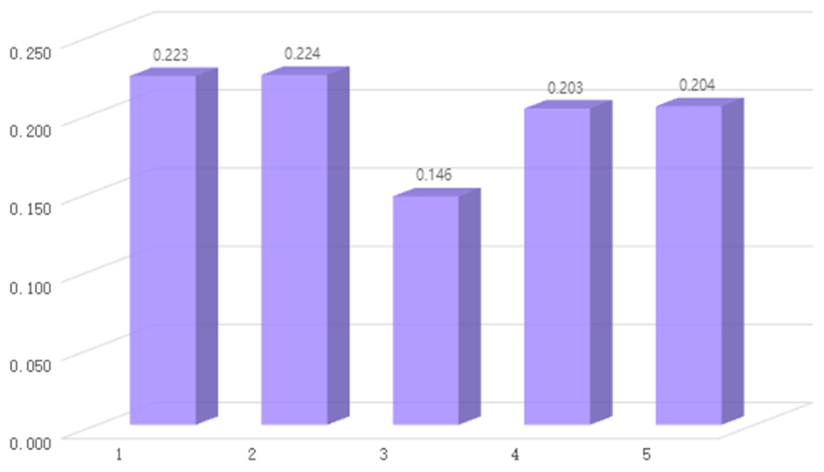
Since $\left\{P_1,P_2,\dots ,P_n\right\}=\left\{0.223,0.224,0.146,0.203,0.204\right\}$, it can be clearly seen from Figure 5 that the optimal alternative is $x_2$.

6. Sensitivity Analysis

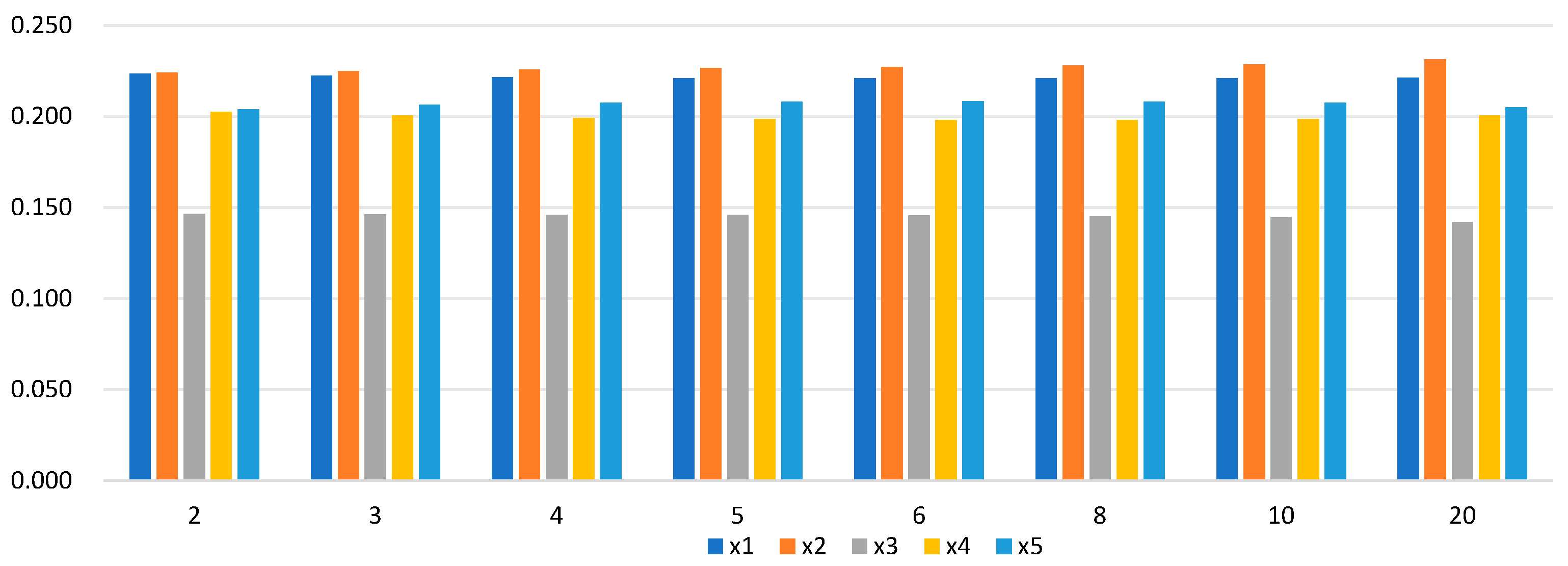
In this section, we will discuss the impact of setting different parameter values q on the results during the q-type semi-dependent neutrosophic decision-making process. The possibility degree values for the candidate alternatives of q (where q ranges from 1 to 10) are presented in

Table 7. Decision results under different parameter values.

$\mathit{q}$	Ranking Vector	Ranking	Best Choice
2	(0.223, 0.224, 0.146, 0.203, 0.204)	$x_2>x_1>x_5>x_4>x_3$	$x_2$
3	(0.222, 0.225, 0.146, 0.200, 0.206)	$x_2>x_1>x_5>x_4>x_3$	$x_2$
4	(0.222, 0.226, 0.146, 0.199, 0.208)	$x_2>x_1>x_5>x_4>x_3$	$x_2$
5	(0.221, 0.226, 0.146, 0.198, 0.208)	$x_2>x_1>x_5>x_4>x_3$	$x_2$
6	(0.221, 0.227, 0.146, 0.198, 0.208)	$x_2>x_1>x_5>x_4>x_3$	$x_2$
8	(0.221, 0.228, 0.145, 0.198, 0.208)	$x_2>x_1>x_5>x_4>x_3$	$x_2$
10	(0.221, 0.228, 0.144, 0.198, 0.208)	$x_2>x_1>x_5>x_4>x_3$	$x_2$
20	(0.221, 0.231, 0.142, 0.201, 0.205)	$x_2>x_1>x_5>x_4>x_3$	$x_2$

and illustrated in Figure 6. As can be seen from Table 7 and Figure 6, although the numerical values of the ranking vector changed, the decision results remained consistent under different parameter values, indicating that the q-type semi-dependent neutrosophic decision model proposed in this article had a strong level of stability. However, the pattern of the changes in the ranking values of the candidate options was not evident. If we only look at the information fusion matrix of experts in Step 2, it can be seen that the value of parameter q exhibits a regular variation in the fusion performed by the q-TSDNWAA operator.

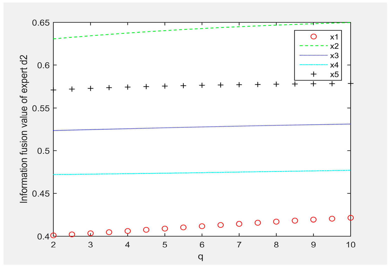
As shown in Figure 7, Figure 8 and Figure 9, when the parameter q gradually increased, the information fusion evaluation score of the q-TSDNWAA operator also increased gradually. Combined with the analysis in Example 1, the parameter q can be regarded as the experts’ attitude toward the decision-making prospect. There was a positive correlation between parameter q and the score value of the q-TSDNWGA operator; as the parameter increased, the decision-maker’s optimistic sentiment increased. On the contrary, when the q-TSDNWGA was used for information aggregation, there was a negative correlation between parameter q and the operator’s score value; as the parameter increased, the decision-maker’s pessimistic sentiment intensified. If the q-TSDNWAA operator is adopted to fuse decision-making information, a higher q value indicates that the decision-maker is more optimistic about the decision-making prospect. If the q-TSDNWGA operator is used for fusing decision-making information, a higher q value indicates that the decision-maker is more pessimistic about the decision-making prospect. Therefore, different decision-makers can select different aggregation operators and appropriate q values according to their own judgments on the decision-making prospects.

7. Comparative Analysis with Other Methods

In this section, we compare the proposed method with existing MAGDM approaches. Two representative types of group decision-making methods are selected for comparison. The first type combines a weighted averaging operator with TOPSIS, as used in references [28,29]; here, we adopt a combination of the q-TSDNWAA operator and TOPSIS. The second type combines arithmetic and geometric averaging operators, as employed in references [30,31,32]; here, we use a combination of the q-TSDNWAA and q-TSDNWGA operators.

As can be seen from

Table 8. Comparison between proposed method and existing methods.

	Refs. [28,29]	Refs. [30,31,32]	Proposed Method
Method	q-TSDNWAA and TOPSIS	q-TSDNWAA and q-TSDNWGA	q-TSDNWAA and Evidence combination
Result	(0.694, 0.757, 0.387, 0.555, 0.482)	(0.627, 0.631, 0.564, 0.523, 0.601)	(0.223, 0.224, 0.146, 0.203, 0.204)
Ranking of alternatives	$x_2>x_1>x_4>x_5>x_3$	$x_2>x_1>x_5>x_3>x_4$	$x_2>x_1>x_5>x_4>x_3$

, both the proposed method in this paper and the methods in the referenced literature identify the second supplier as the optimal choice, which demonstrates the feasibility of the proposed approach. Compared with the other two methods, the proposed method leverages evidence-based information fusion to integrate opinions from different experts in group decision-making, enabling the quantification of credibility and conflict levels, thereby achieving a more comprehensive and reliable overall assessment. It should be noted in the decision-making process that, although increasing the value of q enhances the information representation capability of QTSDNS, the computational complexity of the model also increases. If a decision-making problem involves m attributes, the operators q-TSDNWAA and q-TSDNWGA will perform $m^2+1+2m$ and $2m^2+m+2$ power operations respectively. Therefore, when addressing multi-attribute large-scale group decision-making problems, we recommend the following two approaches to improve the adaptability of the proposed model: First, it is advisable to set the parameter q as a small positive integer, such as 2, 3, or 4. Second, it is recommended to program the model using high-performance computing software like MATLAB R2024b. Additionally, as with most fuzzy multi-attribute decision-making problems, the decision data primarily rely on the objective evaluations of expert panels. Ensuring the objectivity of the data in practical applications is a fundamental prerequisite for scientific and rational decision-making.

8. Conclusions

In this paper, a q-type semi-dependent neutrosophic set (QTSDNS) is proposed. Many traditional fuzzy sets, such as PNS, INS, etc., are special cases of QTSDNS. The significant operational laws of QTSDNS are given. Then, we provided two information fusion tools, q-TSDNWAA operator and q-TSDNWGA operator, and we proved that their fusion of QTSDNN information has good properties. Subsequently, a q-type semi-dependent neutrosophic information group decision-making model is constructed by combining evidence theory with the operators proposed in this paper. Finally, a case study was conducted to select the best laser display technology company for intelligent car manufacturers, demonstrating the effectiveness of the model and analyzing the sensitivity of parameters. In the next step, we will further enrich the theoretical achievements of QTSDNS, provide rules for exponential and integral operations, construct a big data-driven management decision-making methodology system, and combine the latest artificial intelligence technologies to improve the operational efficiency of the model. At the same time, we will further attempt to apply the MAGDM algorithm proposed in this article to areas such as regional new-quality productivity evaluation, comprehensive evaluation of power grid planning schemes, and obstacle judgment in automotive advanced driver assistance systems.

References

1. Alfakeeh, A.S.; Almalawi, A.; Alsolami, F.J.; Abushark, Y.B.; Khan, A.I.; Bahaddad, A.A.S.; Agrawal, A.; Kumar, R.; Khan, R.A. Hesitant Fuzzy-Sets Based Decision-Making Model for Security Risk Assessment. Comput. Mater. Contin. 2022, 70, 2297–2317. [Google Scholar] [CrossRef]
2. Zhang, P.; Zhang, Z.; Gong, D.; Cui, X. A novel normal wiggly hesitant fuzzy multi-criteria group decision making method and its application to electric vehicle charging station location. Expert. Syst. Appl. 2023, 223, 119876. [Google Scholar] [CrossRef]
3. Al Mohamed, A.A.; Al Mohamed, S.; Zino, M. Application of fuzzy multicriteria decision-making model in selecting pandemic hospital site. Future Bus. J. 2023, 9, 14. [Google Scholar] [CrossRef]
4. Feng, J. Multi-attribute perceptual fuzzy information decision-making technology in investment risk assessment of green finance Projects. J. Intell. Syst. 2024, 33, 917–926. [Google Scholar] [CrossRef]
5. Parthasarathy, T.N.; Narayanamoorthy, S.; Thilagasree, C.S.; Marimuthu, P.R.; Salahshour, S.; Ferrara, M.; Ahmadian, A. An enhanced fuzzy IDOCRIW-COCOSO multi-attribute decision making algorithm for decisive electric vehicle battery recycling method. Results Eng. 2024, 22, 102272. [Google Scholar] [CrossRef]
6. Varchandi, S.; Memari, A.; Jokar, M.R.A. An integrated best–worst method and fuzzy TOPSIS for resilient-sustainable supplier selection. Decis. Anal. J. 2024, 11, 100488. [Google Scholar] [CrossRef]
7. Vadivel, K.; Chandrasekar, S.; Deivanayagampillai, N.; Jacob, K. Fuzzy decision-making for cost-effective production planning in manufacturing systems. Eng. Res. Express 2024, 6, 035418. [Google Scholar] [CrossRef]
8. Garg, H.; Khan, F.M.; Ahmed, W. Fermatean Fuzzy Similarity Measures-Based Group Decision-Making Algorithm and Its Application to Dengue Disease. Iran. J. Sci. Technol. Trans. Electr. Eng. 2024, 48, 687–703. [Google Scholar] [CrossRef]
9. Komijan, A.R.; Yazdi, A.K.; Tan, Y.; Ocampo, L.; Nasrollahpourniazi, F. Spherical Fuzzy Multicriteria Decision Making for Evaluating Healthcare Service Quality of Hospitals During the Global Pandemic. Int. J. Comput. Intell. Syst. 2024, 17, 105. [Google Scholar] [CrossRef]
10. Smarandache, F. A Unifying Field in Logics: Neutrosophic Logic; American Research Press: Rehoboth, DE, USA, 1999. [Google Scholar]
11. El, T.Y.; Abdelfattah, W. Feature Imputation using Neutrosophic Set Theory in Machine Learning Regression Context. Eng. Technol. Appl. Sci. Res. 2024, 14, 13688–13694. [Google Scholar] [CrossRef]
12. Zhao, Y. Enhanced exprom methodology using superhypersoft sets for evaluating the quality of cultural industry development in the digital economy with single-valued neutrosophic sets. Neutrosophic Sets Syst. 2025, 79, 19. [Google Scholar]
13. Han, M.; Fan, C.; Huang, S.; Hu, K.; Fan, E. An n-valued neutrosophic set method for the assessment of an offshore oil spill risk. Water Sci. Technol. 2023, 87, 1643–1659. [Google Scholar] [CrossRef]
14. Alpaslan, N. Neutrosophic set based local binary pattern for texture classification.Expert Systems With Applications. Expert Syst. Appl. 2022, 209, 118350. [Google Scholar] [CrossRef]
15. Smarandache, F.; Zhang, Y.; Sunderraman, R. Single valued neutrosophic sets. Neutrosophy Neutrosophic Probab. Set Log. 2009, 4, 126–129. [Google Scholar]
16. Smarandache, F. Degree of Dependence and Independence of the (Sub)Components of Fuzzy Set and Neutrosophic Set. Neutrosophic Sets Syst. 2016, 11, 95–97. [Google Scholar]
17. Bhowmik, M.; Pal, M. Intuitionistic neutrosophic set relations and some of its properties. J. Inf. Comput. Sci. 2010, 5, 183–192. [Google Scholar]
18. Jansi, R.; Mohana, K.; Smarandache, F. Correlation Measure for Pythagorean Neutrosophic Fuzzy Sets with T and F as Dependent Neutrosophic Components. Neutrosophic Sets Syst. 2019, 30, 202–212. [Google Scholar]
19. Feng, X.; Qiu, J.; Wei, C. Assessing Big Data Capabilities in Manufacturing Supply Chains: A Pythagorean Fuzzy MAGDM Framework. Int. J. Fuzzy Syst. 2025, 27, 1279–1302. [Google Scholar] [CrossRef]
20. Choudhary, A.; De, A.; Ahmed, K.; Shankar, R. An integrated fuzzy intuitionistic sustainability assessment framework for manufacturing supply chain: A study of UK based firms. Ann. Oper. Res. 2025, 349, 687–730. [Google Scholar] [CrossRef]
21. Pamucar, D.; Yazdani, M.; Obradovic, R.; Kumar, A.; Torres-Jiménez, M. A novel fuzzy hybrid neutrosophic decision-making approach for the resilient supplier selection problem. Int. J. Intell. Syst. 2020, 35, 1934–1986. [Google Scholar] [CrossRef]
22. Priyadharshini, S.; Mohanaselvi, S. Schweizer-Sklar power aggregation operators based on complex single-valued neutrosophic information using SMART and their application in green supply chain management. Neutrosophic Sets Syst. 2024, 73, 39. [Google Scholar]
23. Riaz, M.; Pamucar, D.; Athar Farid, H.M.; Hashmi, M.R. q-Rung orthopair fuzzy prioritized aggregation operators and their application towards green supplier chain management. Symmetry 2020, 12, 976. [Google Scholar] [CrossRef]
24. Dempster, A.P. Upper and iower probabiiities induced by a muiti-vaiued mapping. Ann. Math. Stat. 1967, 38, 325–339. [Google Scholar] [CrossRef]
25. Wang, N.; Yuen, K.F.; Yuan, J.; Li, D. Ship collision risk assessment: A multi-criteria decision-making framework based on Dempster–Shafer evidence theory. Appl. Soft Comput. 2024, 162, 111823. [Google Scholar] [CrossRef]
26. Ghosh, M.; Dey, A.; Kahali, S. A weighted fuzzy belief factor-based D-S evidence theory of sensor data fusion method and its application to face recognition. Multimed. Tools Appl. 2024, 83, 10637–10659. [Google Scholar] [CrossRef]
27. Huang, Z.L.; Chen, Q.L. Relative possibility relation model for decision making objects with multiple attribute values as interval number and its application. Control Decis. 2022, 37, 1025–1034. [Google Scholar]
28. Mallick, R.; Pramanik, S.; Giri, B.C. Neutrosophic MAGDM based on CRITIC-EDAS strategy using geometric aggregation operator. Yugosl. J. Oper. Res. 2023, 33, 683–698. [Google Scholar] [CrossRef]
29. Nafei, A.; Huang, C.-Y.; Javadpour, A.; Garg, H.; Azizi, S.P.; Chen, S.-C. Neutrosophic fuzzy decision-making using TOPSIS and autocratic methodology for machine selection in an industrial factory. Int. J. Fuzzy Syst. 2024, 26, 860–886. [Google Scholar] [CrossRef]
30. Ye, J.; Yong, R.; Du, S. Multiattribute Group Decision-Making Method in terms of Linguistic Neutrosophic Z-Number Weighted Aggregation Operators. J. Math. 2022, 2022, 9509823. [Google Scholar] [CrossRef]
31. Ashraf, S.; Abdullah, S. Spherical aggregation operators and their application in multiattribute group decision-making. Int. J. Intell. Syst. 2019, 34, 493–523. [Google Scholar] [CrossRef]
32. Liu, P.; Mahmood, T.; Ali, Z. Complex q-rung orthopair fuzzy aggregation operators and their applications in multi-attribute group decision making. Information 2019, 11, 5. [Google Scholar] [CrossRef]
Figure 1. Comparison of constraint ranges for fuzzy sets under different exponents.
Information 16 00742 g001
Figure 2. Aggregated value scores under different q parameters.
Information 16 00742 g002
Figure 3. Visual representation of the methodology’s sequential process.
Information 16 00742 g003
Figure 4. Evaluation system for selecting qualified laser display technology suppliers.
Information 16 00742 g004
Figure 5. Possibility degree values of the candidate alternatives.
Information 16 00742 g005
Figure 6. Calculation results under different parameters q.
Information 16 00742 g006
Figure 7. Information fusion evaluation score of expert d 1 .
Information 16 00742 g007
Figure 8. Information fusion evaluation score of expert d 2 .
Information 16 00742 g008
Figure 9. Information fusion evaluation score of expert d 3 .
Information 16 00742 g009