The Interpretative Effects of Normalization Techniques on Complex Regression Modeling: An Application to Real Estate Values Using Machine Learning

Abstract

The performance of machine learning models depends on several factors, including data normalization, which can significantly improve its accuracy. There are many standardization techniques, and none is universally suitable; the choice depends on the characteristics of the problem, the predictive task, and the needs of the model used. This study analyzes how normalization techniques influence the outcomes of real estate price regression models using machine learning to uncover complex relationships between urban and economic factors. Six normalization techniques are employed to assess how they affect the estimation of relationships between property value and factors like social degradation, resident population, per capita income, green spaces, building conditions, and degraded neighborhood presence. The study’s findings underscore the pivotal role of normalization in shaping the perception of variables, accentuating critical thresholds, or distorting anticipated functional relationships. The work is the first application of a methodological approach to define the best technique on the basis of two criteria: statistical reliability and empirical evidence of the functional relationships obtainable with each standardization technique. Notably, the study underscores the potential of machine-learning-based regression to circumvent the limitations of conventional models, thereby yielding more robust and interpretable results.

1. Introduction

In the actual context of a dynamic and evolving real estate market, the ability to accurately predict property prices is important for subjects like investors, homebuyers, and policymakers. Understanding how property prices are formed aids investors in making informed decisions about purchasing and selling properties. Policymakers use knowledge of price formation to develop regulations that stabilize the housing market to avoid bubbles and crashes, which can have wide-reaching economic impacts. In fact, rapid increases or decreases in housing prices can signal an overheating or underperforming economy, respectively, and they can be used as indicators of economic health. By studying real estate price formation, stakeholders can gain insights into the interactions between demand, supply, economic factors, and expectations that determine property prices. Urban planners and local governments study real estate price trends to make decisions about development, infrastructure investments, and housing affordability programs. The dynamics behind price formation can reveal whether the housing market is efficient or if there are distortions that need to be addressed. Banks and other lenders rely on accurate housing price information to manage risks in mortgage lending and to set appropriate borrowing limits [1].

Regression analysis is utilized to ascertain the extent to which each feature contributes individually to house pricing. An analysis of the housing market and housing price assessment literature reveals two predominant research trends: the application of the hedonic-based regression approach, termed the hedonic pricing model (HPM), and the employment of artificial intelligence (AI) approaches for establishing house price forecasting models. A range of hedonic-based approaches have been employed to investigate the correlation between house prices and their associated effective housing attributes. A comparison of the results of previous studies indicated that the AI technique performed better at forecasting property values than the HPM approach. Machine learning (ML) is a powerful AI approach for predicting property prices and understanding the mechanisms that drive price formation in real estate markets [2]. In particular, ML is a computational method that uses fundamental concepts in computer science in combination with statistics, probability, and optimization to make predictions and improve performance for a given task. ML can be categorized into two types: supervised and unsupervised. In supervised ML, the method receives a dataset with labeled data, making it the most common approach for classification and regression problems. In contrast, unsupervised ML involves data that are not labeled. The overarching objective of ML is to facilitate the creation of efficient and accurate predictions, with two common objectives being classification and regression [3].

The use of ML algorithms provides several advantages; because factors affecting house prices are constantly changing, the developed models can be adapted to new data, making them suitable for dynamic markets and leading to more efficient behaviors of buyers, sellers, investors, and policymakers in their decision-making processes. Unlike traditional valuation methods, such as those based on cyclical capitalization [4], machine learning allows for the detection of complex, non-linear patterns and adaptive modeling in the presence of market uncertainty and low transparency [5]. There are several ML algorithms commonly used for predicting and analyzing real estate prices. Each of them has different strengths, and the choice of the most suitable can depend on the specific attributes of the dataset, the complexity of the modeling task, computational resources, and the level of interpretability required. Data scientists may often test a range of models and use techniques like cross-validation to determine which algorithm performs the best for their specific scenario. For example, linear regression is one of the simplest algorithms and determines the relationship between a dependent variable (e.g., property price) and one or more independent variables (e.g., square footage, bedrooms, etc.) using a linear function [6]. It is easy to be understood and interpreted, but it may not capture complex relationships. Other machine learning algorithms integrate classification and regression for modeling non-linear relationships for finding the hyperplane that best fits the data, as well as handling non-linear relationships using kernel functions, like the support vector machines [7]. Therefore, if the linear regression can be a starting point for understanding relationships in the data, the Random Forest can better capture complex relationships. Support vector machines can be particularly effective when the data have a clear margin of separation. Neural networks, especially deep learning models, are powerful for large datasets with complex patterns, but they require greater computational resources and expertise to train and interpret [8].

However, regardless of the algorithm employed, the accuracy and interpretability of machine learning models are deeply influenced by how the input data are preprocessed. In this context, normalization techniques play a crucial role, especially in regression modeling, where subtle changes in data scale can significantly affect model behavior and output. Although few articles provide unambiguous operational guidelines on the “uses” of standardization techniques, the following are well-documented in the literature:

• Standardization techniques influence the information transmitted to models (e.g., [9,10]);
• The choice of technique may improve or compromise the interpretability of results, particularly in contexts where the semantic meaning of variables is important, such as in economic and social models;
• Different techniques meet different objectives, such as precision, robustness, threshold detection, noise reduction, relative comparison, etc.

This research investigates the impact of six different normalization techniques on the prediction of house prices using a machine-learning-based regression model. The research question addressed in this study is the following: “To what extent do different normalization techniques affect both the statistical reliability and the interpretability of regression models used to predict house prices?”. In order to understand this issue, the analysis is carried out on a heterogeneous dataset consisting of 117 housing prices (as dependent variables) and six extrinsic real estate variables reflecting the social, economic, and environmental characteristics of urban areas in the city of Rome (Italy). Evolutionary Polynomial Regression (EPR), a multivariate supervised regression model, is applied to each normalized dataset. By comparing the statistical accuracy and functional relationships of the resulting models, the study identifies which normalization techniques provide the most robust and interpretable results.

This work contributes to the field of information processes by addressing how the mathematical transformation of variables—through their normalization—affects the structure and the interpretability of the data in urban valuation models. The study responds to the growing need for epistemologically aware data practices in applied machine learning, particularly in socio-economic domains, such as housing market analysis. Even though normalization is usually a mere technical step in statistical modeling, in real estate, its implications are far beyond fixing a scale. For real estate professionals and urban analysts running regression models for forecasting and decision making, the choice of normalization procedure may change the apparent role of explanatory variables and the believability of their relationship with house prices. This paper addresses a need for lessening the chasm between statistical modeling and housing market insights and calls for a scrutiny of the data processing choices not only with respect to statistical integrity but, indeed, with respect to narrative intelligibility.

The reminder of the paper is structured as follows. Section 2 provides a review of the literature on machine-learning-based regression models; Section 3 provides a description of the selected normalization techniques, the sample of real estate data, and the applied ML (i.e., the EPR method) features; Section 4 relates to the results; Section 5 discusses the obtained results; and Section 6 outlines the conclusion and futures insights of the research.

2. Application of Normalization Techniques in the Context of Machine Learning Algorithms and the Real Estate Market

The performance of ML models varies based on many factors, such as the methods of normalization preprocessing. It is not only a technique that is used to convert raw data into a clean dataset, as it also enhances the performance of the analysis. There are dozens of normalization methods in the literature, and no one is the most suitable for all situations. The characteristics of the problem, the predictive task, or the requirements and assumptions of the ML model can guide the choice of an adequate normalization method. Rayu et al. [11] establish that the utilization of these techniques boosts performance by 5–10% in general.

Jo [12] studied the effectiveness of normalization preprocessing of big data to the support vector machine (SVM) as the ML method. Three normalization methods—Simple Feature Scaling, Min-Max, and Z-score—are applied to the SVM for the performance comparison, and the Min-Max normalization method is preferred to the other ones. Pandey and Jain [13] use Z-score and Min-Max as normalization methods for the K-Nearest Neighbors algorithm, a non-parametric method for classification and regression. The average accuracy came out to be 88.0925% for Min-Max normalization and 78.5675% for Z-score normalization. Cabello-Solorzano [14] studied the impact of three normalization techniques, namely, Min-Max, Z-score, and Unit Normalization, on the accuracy of ML algorithms in order to enhance accuracy in problem solving. The results reveal that a few algorithms are virtually unaffected by whether normalization is used or not, regardless of the applied normalization technique.

Eren [2] presents how the ML methods perform with their original values and how the methods react when StandardScaler or MinMaxScaler is used on the dataset for predicting property prices and sale velocities in the real estate market. Zou et al. [15] explore the impact of air pollution on housing prices through an ML approach. The dataset is normalized by using the Min-Max technique for the implementation of the gradient boosting decision tree. Baldominos et al. [16] see the impacts of the use of normalization in the median average error for the different ML techniques considered. Normalization does not have an impact on the ensembles of regression trees, K-Nearest Neighbors, and support vector regression. The only case in which normalization makes a difference is when using a multi-layer perceptron; the median average error increases when normalization (max value) is used. This is contrary to the common belief that normalization is often considered a good practice to prevent numerical instability when training the neural network, but the perceptron is not competitive when compared to other ML techniques in the problem of real estate price prediction. Ekberg and Johansson [17] compare different ML methods’ capability to predict housing prices in the Stockholm city housing market and include a comparison between Random Forest, K-Nearest-Neighbor Regression, and a neural network implementation. The Min-Max scaler is applied to Random Forest implementation, resulting in the one with the best performance. Mu et al. [18] employ Z-score normalization with SVM, least squares support vector machine (LSSVM), and partial least squares (PLS) methods to forecast home values. Muralidharan et al. [19] predict the assessed prices of residential properties by applying ML algorithms (decision trees and Artificial Neural Networks) for the real estate market of Boston. The analyzed numerical data are transformed using Min-Max normalization. Avanijaa [20] proposes a model for house price prediction that assists both buyer and seller. The XGBoost regression algorithm is proposed by normalizing the considered data with the employment of the Z-score technique. Farahzadi et al. [21] try to identify the best model of housing price forecasting using five ML algorithms: the Neighbor Regression Algorithm (KNNR), the Support Vector Regression Algorithm (SVR), the Random Forest Regression Algorithm (RFR), the Extreme Gradient Boosting Regression Algorithm (XGBR), and the Long Short-Term Memory Neural Network Algorithm. The Min-Max normalization method is performed on the housing dataset to obtain the final and error-free version.

In conclusion, the literature highlights the significant but variable impact of normalization techniques on the performance of ML algorithms, particularly in the context of house price forecasting. Although methods like Min-Max and Z-score normalization often improve model accuracy, their effectiveness is not uniform across algorithms and applications. Moreover, some techniques may even introduce bias or reduce interpretability in certain cases, as observed with neural networks or ensemble methods [22]. This variability underlines the need for a specific assessment of the context of standardization strategies. Authors, such as Floridi [23], Bishop [24], and Domingos [25], suggest that preprocessing (including normalization) is not neutral, because it defines the semantic conditions under which a machine learning model learns. So, it is legitimate—and questionable—to reflect on which transformation is more consistent with the objective of knowledge or operation. For these reasons, the present study contributes by offering a comparative assessment of six important normalization techniques within a set of real estate data, applying the Evolutionary Polynomial Regression model to discover how these techniques affect both the statistical accuracy and the interpretative structure of house price forecasts. This approach not only fills a gap in existing research but also provides practical guidance for analysts, policymakers, and urban planners who wish to apply sound and meaningful ML models to the valuation of urban assets.

3. Material and Methods

The present study is composed of six subsequent steps that started with the collection of the sample dependent and independent variables. After that, the initial sample was normalized six times, each of which corresponds to a specific normalization technique. The EPR-ML model was applied to each of the normalized samples in order to obtain six functional models that express the relationships between property prices and the independent variables. Subsequently, the discussion of the results is carried out to highlight the main issues.

3.1. Study Sample

Data collection of independent and dependent variables for the trade areas of the housing market of the city of Rome (Italy) was conducted. The 117 areas cover the entire urban footprint of the city of Rome, including densely populated central areas, suburban zones with varying levels of urbanization, and degraded peripheral districts, reflecting the heterogeneity of the urban fabric (see Figure S1 in Supplementary File). In this case, the dependent variable is the housing quotation provided by the Real Estate Market Observatory of the Revenue Agency for the second semester of 2023. The housing quotation is expressed in unitary terms (EUR/m²). It should be noted that they are not individual transaction data but average values provided by official source. There are six independent variables, and they concern some features of the trade areas for different issues, as follows:

• Presence of degraded neighborhoods (Ad): This is expressed as square kilometers of surface of urban areas that are characterized by the presence of degraded buildings and/or abandoned spaces. The data source is the Italian National Institute of Statistics (ISTAT) and updated to the last release (2021).
• Level of maintenance conditions of buildings (De): This compares the state of conservation of residential buildings in the urban area of interest with the national average value. It is formulated in numerical terms, and the data source is ISTAT and updated to the last release (2021).
• Level of social disease (Ds): This considers the weighted average of several social indicators, such as the employment and unemployment rate and the level of schooling and youth concentration of the urban area. It is formulated in numerical terms, and the data source is ISTAT and updated to the last release (2021) (The social disease index is calculated on the basis of the deviation of four local indicators from the corresponding national average values, recorded by ISTAT in the half year preceding that of the survey. The indicators considered are the unemployment rate, employment rate, youth concentration rate, and education rate. The formula used to calculate the index is as follows: D = 0.40 × (DIS − DISNAZ)+ 0.30 × (OCCNAZ − OCC)+ 0.15 × (GIOV − GIOVNAZ)+ 0.15 × (SCOLNAZ − SCOL). DIS is the local unemployment rate; OCC is the local employment rate; GIOV is the local youth concentration rate; SCOL is the local education rate; and the terms with the suffix NAZ indicate the respective national average values. The coefficients attributed to each indicator reflect the specific weight assigned to each component: 40% to the population is unemployed, 30% to employed, and 15% to young people are concentrated or have an education).
• Resident population (Po): The number of residents living in the trade area. The data source is the latest update of the population census provided by ISTAT in 2021.
• Per capita income (Red): This is defined as the quantity of the average per capita income of people in the trade zone. It is calculated in EUR/year, and it was updated in 2023, as provided by the Economy and Finance Italian Minister.
• Presence of green spaces (V): This represents the square kilometers of the surface occupied by public green parks of the trade area. It is collected by consulting existent urbanistic documents of the soil functions for Rome.

The selected variables are aggregated at the trade zone level. It is important to note that the six independent variables were selected to represent a diverse but significant range of socio-economic and environmental conditions typically used in real estate valuation studies. The choice balances model interpretability, data availability, and the objective of observing how different normalization techniques affect the regression structure when applied to variables with heterogeneous units, intervals, and semantics. The objective is not to model exhaustively all determinants of real estate value but to provide a controlled test bed for assessing normalization effects. It is important to underline that the present study does not have predictive purposes but methodological ones. The six independent variables selected represent an example case of heterogeneous inputs used to evaluate the extent to which normalization techniques influence the automatic construction of the model by the EPR. These variables are also recurrent in the literature on extrinsic value determinants and were chosen to ensure multidimensionality of the regression model inputs, as stated by Chen et al. [26] for per capita income, De Nadai and Lepri [27] for the presence of degraded neighborhoods, Ruggeri et al. [28] for the relevance of maintenance conditions, Naccarato et al. [29] for social issues, Rampini and Cecconi [30] for the population, and Isola et al. [31] for the presence of green spaces. In addition, some literature reviews on the most employed socio-economic and environmental variables used in regression models highlight per capita income, green spaces, population density, and features of the neighborhoods as the most influential factors in the property prices’ formation mechanisms [32,33,34].

Six independent variables were chosen for this study in order to preserve model interpretability and enable a controlled comparison of normalization effects. Despite its apparent modesties, statistical practice fully supports this number; a widely accepted rule of thumb in regression analysis states that in order to ensure statistical robustness and prevent overfitting, a minimum of 10 to 15 observations per independent variable are advised. The current model surpasses the suggested threshold and validates the reliability of the regression results with a ratio of 19.5 observations per variable, despite having only six predictors and 117 observations. In Table S1 of the Supplementary File, the main descriptive statistics of the variables prior to normalization are reported. All variables are expressed in their original units prior to normalization and refer to the year 2021 (or 2023 for per capital income).

The choice of variables with different units and scales is intentional, precisely to analyze how normalization acts on a realistic but heterogeneous sample.

3.2. Normalization

Six different normalization techniques were employed for transforming the initial sample of data collected in the first phase of the approach in order to process the regression and easily compare the results. Among the several normalization techniques, the following six were applied: (i) Min-Max, (ii) max value, (iii) mean value, (iv) sum, (v) standard deviation, and (vi) Z-score non-monotonic. They are chosen as the most frequently employed in regression applications for property prices analysis, according to the reference literature examined in Section 2. In

Table 1. Main features of the six normalization techniques employed.

Normalization Technique	Description	Formula	Type
1. Min-Max	Also known as Min-Max scaling, it is one the most popular and overly used data normalization techniques. It is a technique that linearly transforms the variables, where min and max are the minimum and maximum values of x, where x is the set of observed values. This technique provides normalized values through linear transformation, and it does not change the relative distances between individual data points and so does not alter the data distribution.	z = x − min/max − min	Scaling
2. Max value (Simple Feature Scaling) or maximum absolute scaling	This method rescales values by dividing each observation by the maximum value. This method generates a normalized series with values within the range of 0 to 1.	z = x/max	Scaling
3. Mean value	The normalized value is given as the ratio between the observed value of x and the related mean value	z = x/mean	Scaling
4. Sum	Normalization is performed by dividing each observed datum/value by the sum of values related to the specific data.	z = x/$\sum x$	Scaling
5. Standard deviation	This technique normalizes the data by calculating the standard deviation σ of the observed values x and by dividing each of them to that value.	z = x/σ	Scaling
6. Z-score non-monotonic	Also called standardization, Z-score normalization sees features rescaled in a way that follows thee standard normal distribution property with μ = 0 and σ = 1, where μ is the mean (average) and σ is the standard deviation from the mean.	z = $e^{{\displaystyle \frac{{\left(x-\mathsf{\mu }\right)}^2}{{\mathsf{\sigma }}^2}}}$	Not Scaling

, each normalization technique is briefly described, and the related formulas and type (if scaling or not) are reported.

Classification of normalization techniques can be performed through various approaches. The most common classifications in the literature are performed according to the (i) distance measurements, (ii) linearity of the normalization process, or (iii) optimization orientation of the values. For normalization processes that are not based on distance, a specific value is used. For the techniques in this category, maximum value, minimum value, mean value, standard deviation, reference (ideal/target) value/range, adjustable constant number, and data distributions are used in the normalization process [35].

The linearity of the normalization process means that the utilities or values in the criterion increase or decrease monotonously in a specific direction. In non-monotonic normalization processes, there is no continuous increase or decrease of acceptable performance values in a certain direction. Some reference-based normalizations and non-linear normalizations, such as Z-score non-monotonic, are examples of non-monotonic normalization techniques.

Scalar normalization preserves the relative relationships between the data, scaling them into a certain range but preserving the proportional relationship between the original values. It avoids variable size problems, especially when some variables have very different orders of magnitude (e.g., square meters and prices in euros). Generally, it is useful for machine learning algorithms that may be influenced by different variables. Non-scalar normalization, like Z-score non-monotonic, transforms data to fit a particular distribution by changing the shape of the original distribution through a non-linear transformation. This introduces non-monotonic behavior, i.e., the relative order of values can change because values further from the mean undergo an exponential transformation that disproportionately enhances the extremes.

3.3. Machine Learning Application

Once the six normalized study samples were obtained, the investigation of the effects on property price prediction was carried out by processing each of them with a machine learning method, specifically, the EPR. This method applies to an evolutionary multi-objective genetic algorithm as an optimization strategy based on the Pareto dominance criterion. In particular, it is able to (i) maximize the statistical accuracy, (ii) minimize the number of terms (i.e., the model’s parsimony), and (iii) maximize the readability through the minimization of the number of the explanatory variables of the regression equation. The optimization strategy provides for a set of Pareto front of optimal models for the three objectives considered. The following equation (Equation (1)) summarizes a generic non-linear model structure implemented in EPR:

$$Y=a_0+{\displaystyle \sum _{i=1}^n[a_i\cdot {(X_1)}^{(i,1)}\cdot \dots \cdot {(X_j)}^{(i,j)}\cdot f({(X_1)}^{(i,j+1)}\cdot \dots \cdot {(X_j)}^{(i,2j)})]}$$

(1)

where

• a₀ is the constant additive term that comprises the bias;
• n is the number of additive terms (with the constant additive term excluded);
• a_i is the numerical coefficient generated for each additive term;
• X_i is the explanatory variable selected by the model;
• (i, l)—with l = (1, …, …, 2j)—is the exponent of the l-th variable within the i-th additive term. It is selected from a range of real numbers;
• f is a function selected by the user from a set of mathematical expressions.

The ML method provides for an equation that relates the dependent variable of the housing quotation with the independent variables selected by the algorithm as capable of explaining the property price. The equation is characterized by a certain level of algebraic complexity, a number of explanatory variables, and a specific degree of statistical performance expressed by the coefficient of determination (CoD), calculated as shown (Equation (2)):

$$COD=1-{\displaystyle \frac{N-1}{N}}\cdot {\displaystyle \frac{{\displaystyle \sum _N{(y_{estimated}-y_{detected})}^2}}{{\displaystyle \sum _N{(y_{detected}-mean(y_{detected}))}^2}}}$$

(2)

where y_e is the assessed values of the dependent variable by the EPR technique, y_d is the collected values of the dependent variable, and N is the sample size.

4. Results

The iterative application of the EPR-ML method is carried out with the same settings for each of the normalized study samples processed. In particular, the EPR is implemented with a statical regression (not lag), no inner function f selected, a maximum number of equation terms equal to nine, and a set of exponents belonging to the range (0, 0.5,1, 1.5, 2). The exponent equal to 1 means that the model considers the variable in its original form, the exponent equal to 0 means that no variable is considered, the exponent equal to 2 means it is elevated to the square, and, if it is equal to 0.5, it makes the square root.

The models generated by the EPR method for each elaboration (normalization technique employment) are reported in

Table 2. Regression models of EPR by varying the applied normalization technique.

Normalization Technique	EPR Model	CoD
Min-Max	Y = +14,148.42Red0.5V0.5+ 4999.60Red1.5 − 25,443.52Red2V − 17,471.39Pop0.5V0.5 + 46,086.70Pop1.5V0.5 − 36,408.12Pop2V0.5 + 3588.35Ds0.5Pop0.5Red0.5 − 2248.12DsRed0.5 + 1631.91	92.56
Max value	Y = +11,502.39V0.5 + 8002.41Red − 54,382.38Pop0.5V0.5 + 86,448.17PopV0.5 − 45,878.21Pop1.5V0.5 + 732.06Ds0.5 − 10,810.62Ds0.5Red1.5 + 20,943.46Ds0.5Pop0.5Red2 − 274,967.54Ad2Ds1.5De1.5V2 − 167.16	93.14
Mean value	Y = +4153.04V0.5 + 2478.67Red − 9396.33Pop0.5V0.5 + 7145.31PopV0.5 − 1805.52Pop1.5V0.5 + 0Ds0.5V0.5 − 647.53Ds0.5Red1.5 + 469.63Ds0.5Pop0.5Red2 − 5.48Ad2Ds1.5De1.5V2 + 206.42	93.05
Sum	Y = +29,1197.96Red − 4103,147,932.81De0.5Red1.5V2 + 55,369.48Ds0.5V0.5 − 918,096.85Ds2 + 315,533,225.62Ad0.5De1.5Red − 187,340,817.60AdDe0.5PopV0.5 + 406,811,293,021.87Ad1.5Ds0.5Pop0.5Red2 − 692,800,296,667.61Ad1.5DsDe0.5Red1.5 + 111,615,175,283.57Ad2Ds2De0.5 − 35.8226	92.07
Standard deviation	Y = − 78.9271Red0.5V1.5 + 1177.58Red + 824.44Ds0.5 + 2122.01Ds0.5V0.5 − 518.3147Ds0.5Red − 1447.68Ds0.5Pop0.5V0.5 + 31.38Ds0.5PopRed2 + 12.65Ad0.5DePop2Red0.5V1.5 − 11.21Ad2De2V1.5 − 428.77	92.37
Z-score non-monotonic	Y = − 9827.24V1.5 + 7514.77V2 − 7238.88Red − 8995.01Ds2Red0.5 + 10,176.16Ds2Red1.5 − 1705.87Ad0.5 + 2732.09Ad0.5Red2V + 10,849.70	75.21

.

The statistical significance of the obtained models is very high for all (CoD > 92.00). Only for the Z-score non-monotonic normalization is the CoD slightly lower, but it still gives a good statistical significance of the results. For the max value (or maximum absolute scaling) normalization the CoD of the selected model, no. 27 is the highest one, followed by model no. 31 of the mean value’s normalization (CoD = 93.05).

As can be seen in Table 2, the models are characterized by a different set of explanatory variables. In most cases, all of them are present in the model, except for the presence of degraded neighborhoods [Ad] that is missing in the model of the Min-Max technique. Also, the level of maintenance conditions of buildings [De] is excluded by the generated results for the models of Min-Max and Z-score non-monotonic techniques. The level of social disease [Ds] is not taken into account in the model of the standard deviation technique. Instead, the resident population variable [Po] is excluded from the Z-score non-monotonic chosen model. In

Table 3. Included and excluded independent variables.

Normalization Technique	Presence of Degraded Neighborhoods [Ad]	Level of Maintenance Conditions of Buildings [De]	Level of Social Disease [Ds]	Resident Population [Po]	Per Capita Income [Red]	Presence of Green Spaces [V]
Min-Max	x	x	✔	✔	✔	✔
Max	✔	✔	✔	✔	✔	✔
Mean value	✔	✔	✔	✔	✔	✔
Sum	✔	✔	✔	✔	✔	✔
Standard deviation	✔	✔	x	✔	✔	✔
Z-score non-monotonic	✔	x	✔	x	✔	✔

Note: “×” indicates that the variable was automatically excluded from the final EPR model using the specific normalization technique in that column. The same variable may still be included in models based on other techniques and is analyzed accordingly in the discussion.

, a synthesis of the included and/or excluded independent variables for each normalization technique’s model is shown.

As correctly observed in the literature [36,37,38,39], normalization is carried out on independent variables; therefore, it does not alter the regression algorithm, nor does it affect the calculation of the coefficient of determination (R²), and it does not change the sign of the coefficients. However, in the case of the non-linear and adaptive EPR method, which constructs the shape of the equation as a function of the input data, normalization can have a substantial impact on the final result. Although the algorithm remains formally unchanged, normalization does the following:

• It changes the distribution and variance of independent variables;
• It alters the correlations between variables;
• It influences the probability that some variables are selected in the early stages of the evolutionary algorithm;
• It can lead to the selection of different combinations of terms and powers;
• It therefore produces different final equations, with potentially different R².

In other words, normalization does not change the structure of the algorithm, but it affects its adaptive behavior within user-defined boundaries. This effect is not an anomaly but a systemic feature of non-linear data-driven models, such as EPR, neural networks, or boosting.

Table 4. Clarification of which components of the regressions are preserved or altered by normalization.

Regression Component	Affected by Normalization?	Explanation	References
Coefficient dimension	Yes	Normalization changes the scale of the variables, thus rescaling the coefficients accordingly.	Huang et al., 2023 [36] Ioffe and Szegedy, 2015 [37] Sammut and Webb, 2017 [38] de Amorim et al., 2023 [39]
Coefficient sign (directionality)	No	Not always true. In linear models, yes, but in symbolic non-linear models (EPR, GEP), normalizing can change the selection of variables or the equation itself, and even the sign can change.
Units of coefficients	Yes	After normalization, coefficients no longer refer to original units (e.g., EUR/m2, inhabitants).
R2 (coefficient of determination)	No	In fixed and linear models, this is true. But, in adaptive, non-linear models, such as EPR, normalization can change the equation, so R2 can also be affected.
Variable importance (relative impact on the dependent variable)	Yes	Normalization can alter the relative weight of variables in the model, affecting their selection.
Model structure (equation form)	No (in most cases)	Only for fixed and linear models. In EPR, DNN, etc., normalization can radically change the structure of the equation.

below summarizes these differences, distinguishing the expected behavior in linear models from that observable in adaptive models.

5. Discussion

The study of the effects of normalization techniques on the regression’s results can be performed by analyzing three main aspects: (i) the type of functional relationship with the dependent variable, (ii) the trend, and (iii) behavior interpretation. The first aspect led to the identification of (i) increasing and/or decreasing, (ii) linear positive and/or negative, and (iii) non-linear or quadratic functional relationships between the property price and each independent variable admissible. The importance of this aspect relates to four issues: consistency of results, interpretability, robustness of the model, and generalizability. Standardization techniques can change the distribution of independent variables and thus alter their impact on house prices. If the functional relationship between price and an independent variable changes significantly after normalization, it is necessary to understand whether the change is real or an artefact of data transformation. In other words, it is essential to know whether the normalization process is fattening the outliers or distorting the variables. If the form of the functional relationship is altered by standardization, the economic and urban significance of the variables may be compromised, making it difficult to draw practical conclusions and interpretations. In addition, some normalization techniques may lead to the exclusion of significant variables, affecting the robustness of the regression model and the number of variables selected. If a normalization technique reduces the variance of a variable to make it statistically irrelevant to the regression, this variable could be automatically excluded from the model (as in Min-Max scaling for variables with very small ranges). Identifying the nature of the functional relationship helps to understand whether a variable has been excluded because it is actually irrelevant or because normalization has altered its information. Correct identification of the functional relationship therefore helps to select the most appropriate normalization technique to maintain the validity of the forecasts.

Trend identification allows us to understand how independent variables influence the price of real estate. When comparing six different normalizations, it is important to check that the relationship between the exogenous variable and the price remains constant in direction and strength. If one normalization technique drastically changes the slope of the functional relationship compared to the others, this may indicate that it is altering the economic significance of the variable. This is essential to ensure that the results obtained after standardization are consistent with market reality. If per capita income has a positive and increasing relationship with price in all normalization techniques except one (e.g., Z-score non-monotonic), which instead shows a non-linear trend with an initial fall and then a rise, this means that this technique has introduced bias into the model. Trend (slope) analysis makes it possible to identify the standardization techniques that accentuate or attenuate the effects of variables, thus helping to select the most appropriate method according to the objective of the study.

Finally, the analysis of the interpretation of the behavior between the dependent and independent variables has practical implications for policymakers, investors, and planners. If the model leads to misinterpretations of the relationships between variables, decisions based on these results may be wrong. For example, if the model suggests that housing density is always negative for property values, this could lead to policies that limit the construction of new units. However, if a different standardization technique shows that the relationship becomes positive beyond a certain threshold, then it may make sense to promote urban densification strategies. The interpretation of the behavior of the variable helps to choose the technique of normalization that best preserves the economic logic of the phenomenon studied. In

Table 5. Level of social disease’s results.

Min-Max
	Type of functional relationship with the dependent variable: Parabolic ratio with concave down (U inverted). Trend: Generally decreasing and parabolic with low slope (−11.43). Initially, if the level of social disease increases, passing from 1.14 to 7.04, the housing quotation also increases +4.26%, then slightly decreasing by −21.83% when the level of social disease is the maximum retrieved. Behavior interpretation: At low levels of social distress, the house price may increase slightly. Beyond a critical threshold (7–10), the effect becomes negative, and the price starts to fall. For very high levels of social distress (>20–30), the price decline is accentuated, reflecting a context of degradation and low attractiveness for the property market.
Mean value
	Type of functional relationship with the dependent variable: Non-linear decreasing relationship with hyperbolic trend. Trend: Decreasing and parabolic with medium slope (−55.76). An increase in the level of social disease generates a reduction of housing values equal to −13.65% when the level of social disease is maximum. The trend thus shows an initial phase of high price sensitivity to social distress, followed by a reduction with a more contained effect. Behavior interpretation: Housing values rapidly diminish if there are high levels of social disease. In areas with low levels of social deprivation, the negative effect on house prices is strong, suggesting that initial changes in the level of social deprivation are perceived strongly by the housing market. Once a certain threshold is reached, the relationship remains negative, but price changes are more muted.
Z-score non-monotonic
	Type of functional relationship with the dependent variable: Parabolic with non-linear decreasing relationship. Trend: Decreasing with progressive acceleration and high slope (−772.14). An increase in the level of social disease generates a reduction of housing values equal to −43.33% when the level of social disease is maximum. Behavior interpretation: Increasing sensitivity of the property market to the deteriorating social environment. At high values, the curve suggests an accelerated decline in property values, suggesting that areas of high social deprivation are experiencing a significant loss in property values.
Sum
	Type of functional relationship with the dependent variable: Decreasing parabolic ratio with downward concavity (inverted U). Trend: Generally decreasing and parabolic with a maximum reached in correspondence to a level of social disease equal to 5.31. Further growth of the variable produces a reduction of property values up to −44.45%. Non-linear double-phase trend: initial growth followed by progressive decline. Behavior interpretation: In areas with very low social distress, the housing market does not perceive discomfort as a negative factor. After a critical threshold, the market reacts negatively; prices start to fall, indicating that increased discomfort reduces the attractiveness of residential and real estate. For high values, the price continues to fall but with a less steep slope, suggesting a saturation effect.
Max value
	Type of functional relationship with the dependent variable: Non-linear decreasing hyperbolic relationship. Trend: Decreasing with negative progressive slope (−307.63). Each increase of the variable produces an average reduction of the property value equal to −0.26%. Behavior interpretation: For low levels of social distress, the housing market reacts very sensitively, with an immediate reduction in prices, signaling that even small signs of social distress can negatively impact housing demand.
Standard deviation
	Type of functional relationship with the dependent variable: Non-linear increasing hyperbolic relationship. Trend: Increasing progressive acceleration with positive slope (797.56). An average growth equal to 1.40% is generated by the i-th increase in the social disease level. Behavior interpretation: The graph shows a counter-intuitive behavior. If the relationship is real, it might suggest that social distress is not perceived as a negative factor by investors or that areas with high levels of distress have a property market driven by particular dynamics (for example, gentrification or real estate speculation).

,

Table 6. Resident population’s results.

Min-Max
	Type of functional relationship with the dependent variable: Non-linear and non-monotonous relationship with double trend reversal. Trend: Decreasing with stabilization and subsequent reduction. Values of the dwellings decrease on average by −1.84% if the resident population increases to the 18,000 units, and, if they are greater than 31,000 units, an average decrease of the values is observed (−0.46%). In the range between 18,000 and 31,000 units, the values of the dwelling slightly increase on average by +0.21%. Behavior interpretation: Low-density areas are characterized by exclusivity, while population growth can induce a saturation effect. A moderate density of dwellings has been demonstrated to have a positive effect on property value, likely due to the presence of services, infrastructure, and sustained housing demand. However, above a critical density threshold, the effect becomes negative, probably due to livability problems and congestion.
Mean value
	Type of functional relationship with the dependent variable: Non-linear decreasing relationship with hyperbolic effect. Trend: Descending with high initial slope and subsequent flattening. The trend is characterized by a persistent decline, accompanied by an initial intense price reduction that subsequently stabilizes, leading to a more gradual decline in areas exhibiting higher density. Behavior interpretation: The housing market demonstrates a propensity to reward low-density areas, albeit to a limited extent. Moderate-density areas have been observed to exhibit price stability, while high-density areas have been shown to undergo a gradual devaluation.
Sum
	Type of functional relationship with the dependent variable: Parabolic ratio with concave downward (U inverted). Trend: Initial growth followed by a gradual decline. If the inhabitants are less than 14,000, the housing values increase by +1.95%. Instead, overcrowding of more than 14,000 inhabitants negatively affects housing values. Behavior interpretation: The housing market demonstrates a clear preference for areas characterized by moderate densities of dwellings. Conversely, areas exhibiting very low or very high densities are deemed less desirable, likely due to divergent factors (exclusivity in low density areas and congestion in high density areas).
Max value
	Type of functional relationship with the dependent variable: Non-linear decreasing relationship with hyperbolic effect Trend: Decreasing with rapid initial descent and subsequent stabilization. Property values decrease by −47.49% if the resident population increases to 19,000 units, and, if they are greater than 46,000 units, they decrease by −20.25%. In the range between 19,000 and 46,000 units, the values of the dwellings slightly increase by an average of +7.91%. Behavior interpretation: In the initial phase of urban development, low-density areas typically exhibit higher property prices, which subsequently experience a rapid devaluation as the population grows. Moderate density areas, on the other hand, demonstrate a tendency to stabilize prices. However, when the density of dwellings exceeds a certain threshold, a second phase of real estate depreciation ensues.
Standard deviation
	Type of functional relationship with the dependent variable: Non-linear decreasing relationship with hyperbolic effect. Trend: Decreasing with a rapid initial fall, followed by stabilization and a slight recovery of the decline. An average growth equal to 3.99% is generated by the i-th increase of the resident population. Behavior interpretation: In the initial phase, low-density areas exhibit higher prices, but as population growth accelerates, a process of rapid devaluation ensues. Moderate-density areas, on the other hand, demonstrate a tendency to maintain more stable prices. However, when density levels exceed optimal thresholds, a new phase of devaluation commences.

,

Table 7. Per capita income results.

Min-Max
	Type of functional relationship with the dependent variable: Increasing non-linear relationship with downward concavity (saturation effect). Trend: High slope (5754). There is an average growth equal to 1.95% by the i-th increase of resident population. Evidence suggests that the variable is increasing; however, the effect on real estate prices gradually diminishes as the value of the variable rises. Behavior interpretation: The increase in the per capita income has a positive effect on real estate values, but with decreasing marginal returns.
Mean value
	Type of functional relationship with the dependent variable: Non-linear increasing with progressive acceleration. Trend: Increasing, with a noticeable acceleration in the final phase. Behavior interpretation: The initial increases in per capita income have been shown to exert a limited effect on real estate prices. However, once a certain economic threshold of approximately EUR 30,000 has been attained, the impact becomes more pronounced. Furthermore, an increase in per capita income exceeding EUR 50,000 has been demonstrated to result in a significant acceleration of real estate prices.
Z-score non-monotonic
	Type of functional relationship with the dependent variable: Non-linear decreasing with hyperbolic effect and final inversion. Trend: Decreasing with stabilization and subsequent slight inversion. Behavior interpretation: Property values are negatively affected by the per capita income if it is less than EUR 26,000/per capita. Evidence suggests that the hypothetical negative effect of per capita income on the housing market may not be permanent, as the presence of a possible stabilization phase and a slight recovery indicate.
Sum
	Type of functional relationship with the dependent variable: Linear direct proportionality. Trend: Increasing and positive. Behavior interpretation: Property values rise with the growth of the per capita income.
Max value
	Type of functional relationship with the dependent variable: Linear increasing. Trend: Linear and constantly increasing.Behavior interpretation: An increase in per capita income will lead to a proportional increase in the value of real estate. Furthermore, the absence of critical thresholds or variations in the growth rate suggests that the real estate market responds consistently to per capita income growth.
Standard deviation
	Type of functional relationship with the dependent variable: Non-linear increasing with progressive acceleration. Trend: Growing, with acceleration in the final phase. Behavior interpretation: The initial increases in per capita income have been shown to exert a limited effect on real estate prices. However, once a certain threshold (~EUR 30,000) has been reached, per capita income begins to have a more significant influence on the value of real estate. Furthermore, over EUR 50,000, the acceleration suggests increased demand and potential speculative effects.

,

Table 8. Presence of green spaces results.

Min-Max
	Type of functional relationship with the dependent variable: Non-linear with saturation effect (downward concavity, plateau shape). Trend: Initial growth followed by stabilization and slight decline at the end. Evidence of a saturation effect is demonstrated, accompanied by a minor inversion at the conclusion. Behavior interpretation: Having a lot of green spaces around makes house prices go up, but only to a certain point. The best amount of green spaces is between 0.10 and 0.50. Too many green spaces could make house prices go down.
Mean value
	Type of functional relationship with the dependent variable: Non-linear with saturation effect (inverted u-curve with minimal variation). Trend: Inverted U with minimal variation. The housing quotation rises when the presence of green spaces is less than 0.23 km2. Behavior interpretation: The notion that an increase in green space is perceived as a market advantage is only partially substantiated. The positive effect of green space on property value is found to be limited and tends to stabilize rapidly. An excess of green space could therefore have a neutral or slightly negative impact.
Z-score non-monotonic
	Type of functional relationship with the dependent variable: Non-linear decreasing with final reversal effect. Trend: The data show a decrease, with a slight recovery in the final phase. Behavior interpretation: The presence of a greater quantity of green space has been demonstrated to be positively correlated with the property value of residential properties. However, an increase in green space to a certain extent has been shown to be associated with a devaluation of the property. Beyond a certain limit, there is a slight recovery in property value, suggesting that an abundance of green space may be a positive factor in specific contexts.
Sum
	Type of functional relationship with the dependent variable: Non-linear with threshold effect (inverted u-curve). Trend: Upside down (growth followed by gradual decline). Behavior interpretation: The impact of green spaces on real estate prices is an area of interest for researchers. It is evident that green spaces have a positive effect on real estate prices up to a certain point. However, once a threshold of 0.40 is passed, their impact becomes less relevant or even slightly negative.
Max value
	Type of functional relationship with the dependent variable: Non-linear increasing with progressive acceleration. Trend: Positive slope (8419). There is an average growth equal to 15.45% by the i-th increase of green spaces. The rate of increase accelerates in the advanced phase. Behavior interpretation: Green spaces have a positive and growing impact on real estate value. The effect becomes particularly strong when the area of green spaces exceeds 0.20–0.30 km2. Areas with more green can be perceived as exclusive and high-value.
Standard deviation
	Type of functional relationship with the dependent variable: Increasing non-linear with acceleration effect. Trend: Increasing with initial acceleration and maintenance of growth rate. There is an average growth of 5.55% for every i-th increase of green spaces. Behavior interpretation: The increase in green spaces has an immediate and significant positive effect on real estate prices.

,

Table 9. Presence of degraded neighborhood results.

Mean value
	Type of functional relationship with the dependent variable: Slightly decreasing linear. Trend: Slightly decreasing. There are no acceleration points or inversions, indicating a stable and constant relationship. Behavior interpretation: An increase in the degraded area is associated with a slight decrease in the value of real estate. Urban degradation has a negative effect, but its impact is marginal.
Z-score non-monotonic
	Type of functional relationship with the dependent variable: Slightly decreasing linear. Trend: Linear and constantly decreasing. Each increase of the variable produces an average reduction of the property value equal to −0.15%. Behavior interpretation: Degraded neighborhood surface has a continuous and predictable negative effect on property value.
Sum
	Type of functional relationship with the dependent variable: Non-linear, slightly decreasing, with a more pronounced initial decline. Trend: Decreasing, with a more steep initial phase followed by stabilization. Behavior interpretation: The presence of degradation exerts an immediate effect on the perception of real estate value, precipitating a more pronounced devaluation in the early stages. Subsequent to this, the market tends to stabilize, and devaluation becomes more gradual.
Max value
	Type of functional relationship with the dependent variable: Slightly decreasing, linear. Trend: Slightly decreasing and constant Behavior interpretation: As the degraded surface increases, property values decrease very gradually. This indicates that urban degradation is perceived as a negative factor, but it is not the main determinant of real estate prices.
Standard deviation
	Type of functional relationship with the dependent variable: Slightly decreasing, linear. Trend: Slightly decreasing and constant with negative slope. Behavior interpretation: Urban degradation always has a negative impact on real estate prices, but without extreme effects.

and

Table 10. Level of maintenance conditions of buildings results.

Mean value
	Type of functional relationship with the dependent variable: Slightly decreasing. Trend: Very slight and gradual. Behavior interpretation: The relationship between degraded building conditions and housing quotation is negative, indicating that as the deterioration of buildings increases, the value of real estate tends to decrease.
Sum
	Type of functional relationship with the dependent variable: Non-linear with intermediate minimum and final growth. Trend: Initial decrease, intermediate minimum and final increase. Behavior interpretation: The relationship between maintenance conditions of buildings and housing quotation is non-linear and follows a U-curve, suggesting that buildings with moderate deterioration (intermediate index values) have the lowest values, whereas those with very good or very bad maintenance conditions have higher values. The U-effect suggests that moderately degraded properties are less attractive to the market.
Max value
	Type of functional relationship with the dependent variable: Slightly decreasing and linear. Trend: Slightly decreasing and constant. Behavior interpretation: The deterioration of buildings is associated with a depreciation of real estate, but the effect is very weak and gradual.
Standard deviation
	Type of functional relationship with the dependent variable: Inverted U-ratio (non-linear with intermediate maximum and final decline). Trend: Inverted; initial growth, intermediate maximum, final decline. property values increase if the level of maintenance conditions of buildings is less than 2.98. Behavior interpretation: Moderately degraded properties appear to have higher demand than poor or perfect condition.

, all of the three mentioned aspects of regression results are discussed for each of the independent variables and normalization techniques.

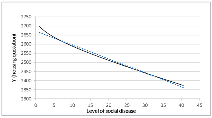
The majority of the techniques demonstrate a negative relationship between social distress and real estate value, which is consistent with the expected economic dynamics. However, with the exception of the standard deviation technique, which indicates an increase in real estate values as social unrest escalates, the remaining techniques exhibit an initial phase where social distress does not exert a negative influence (or even promotes a slight increase in prices), followed by a phase of marked decline beyond a critical threshold. These techniques have the potential to accentuate the significance of critical thresholds, thereby rendering the model more susceptible to variations in data. Conversely, mean value, Z-score non-monotonic and max value scaling techniques have been observed to confirm a consistent decline in real estate prices with an increase in social distress. These techniques appear to be the most reliable in representing a constant devaluation without emphasizing critical thresholds. The standard deviation scaling technique, which alternates the effect of the relationship, has been observed to demonstrate a growing trend, with an increase in price concomitant with an increase in social discomfort. However, it is important to note that this technique may distort the scale of the data, reversing the sign of the relationship. Standard deviation scaling has also been observed to change the ranking of observations, giving more weight to extreme values, leading to an inversion of the relationship between social distress and real estate price. This has resulted in a disproportionate amplification of the weight of observations with high social discomfort, distorting the relationship between variables. This effect could be particularly pronounced in specific markets, such as areas experiencing high social distress that are subject to speculative investment or gentrification processes. In such cases, an increase in prices may be observed despite the associated degradation. Consequently, mean value and max value scaling are considered the most reliable options. However, if the analysis aims to identify a critical threshold, Min-Max scaling and sum show threshold effects in social distress.

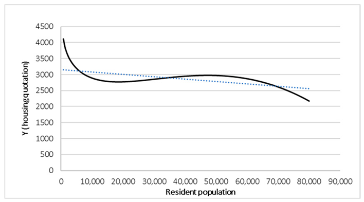
All techniques indicate that property values tend to decrease with an increase in the resident population, albeit with discrepancies in the mode of this devaluation. Min-Max, mean value, max value, and standard deviation demonstrate a pronounced initial devaluation, followed by a stabilization phase and then a slight descent in high density areas. Sum scaling exhibits a reverse U-shaped trend, suggesting that moderate housing density may be associated with higher property values prior to a subsequent devaluation. Min-Max scaling, mean value scaling, max value scaling, and standard deviation scaling demonstrate a rapid devaluation in the initial population levels, followed by a stabilization phase. Notably, Min-Max and standard deviation scaling exhibit a slight decline in the final phase, suggesting a negative impact of high density. Conversely, mean value and max value scaling show a sharper stabilization, indicating the potential for high density areas to maintain stable prices. Sum scaling is the only technique that shows an initial increase in real estate value in sparsely populated areas, followed by a gradual decline of over 30,000 inhabitants. This normalization emphasizes the threshold effect, highlighting the optimal value of housing density before devaluation. It is evident that there are discrepancies in the behavior of the more than the 60,000 resident population under consideration. Min-Max and standard deviation demonstrate a recovery in the devaluation of the subjects, suggesting that urban congestion could potentially impact property value. Conversely, mean value and max value show greater stabilization, indicating that, under these normalizations, high density is not inherently detrimental. Conversely, sum scaling demonstrates a progressive decline without a discernible stabilization phase, underscoring the adverse relationship between housing density and real estate value. In conclusion, mean value scaling and max value scaling emerge as the most reliable for a constant and predictable depreciation, while sum scaling is more suitable as it exhibits the U-shaped behavior. When the objective is to emphasize the impact of high density on final devaluation, Min-Max scaling and standard deviation scaling prove to be more sensitive in areas with over 60,000 inhabitants.

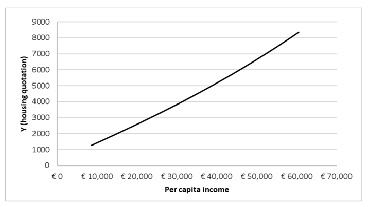
The majority of the techniques indicate a positive correlation between per capita income and property value, though the specific patterns of growth and acceleration vary across techniques. Notably, Z-score non-monotonic demonstrates an initial decrease, followed by a recovery in the final phase. The overall positive correlation between per capita income and real estate value is substantiated; however, the influence of per capita income on real estate growth exhibits variations in its implementation across different techniques of normalization. The Z-score non-monotonic normalization may have accentuated an initial rebalancing effect that is not evident in other techniques. Sum scaling is the sole technique that demonstrates a perfectly linear relationship between per capita income and real estate value, suggesting that it may be the most suitable normalization method if one aims to model a linear behavior devoid of threshold or acceleration effects. However, it is noteworthy that per capita income may exerts a limited impact in the nascent stages of economic development, yet it becomes increasingly significant as the economy matures. Conversely, mean value, max value, and standard deviation scaling demonstrate an escalating relationship with progressive acceleration. It is conceivable that the effect of the per capita income is not invariably positive and that critical thresholds exist: Min-Max scaling may emphasize a threshold beyond which further increases in the per capita income do not have a strong impact on real estate growth; Z-score non-monotonic might suggest that in less developed economies the per capita income could initially reduce property values, and then support them at a later stage. In summary, the demonstration of linear growth can be achieved through the utilization of sum scaling. The role of the rising of per capita income on real estate values is illustrated by mean value, max value or standard deviation scaling. Finally, potential threshold or saturation effects are emphasized by Min-Max scaling (saturation) or Z-score non-monotonic (initial inversion phase).

The majority of the techniques examined demonstrated a positive correlation between green spaces and property value, though variations in growth rate and saturation effects were observed. Notably, Z-score non-monotonic exhibited an initially decreasing relationship, followed by a slight recovery in the final phase. The overall conclusion of the study suggests a positive relationship between green spaces and real estate value. Conversely, Min-Max scaling, mean value scaling, and sum scaling demonstrate a reverse U-shaped relationship, indicating that green spaces exert a positive effect up to a certain threshold, beyond which they can potentially have a neutral or negative impact. These normalizations underscore an optimal threshold between green and real estate value. Max value scaling and standard deviation scaling reveal a steady growth in real estate value with an increase in green. Z-score non-monotonic, on the other hand, demonstrates an initial devaluation, followed by a subsequent reversal. This standardization is particularly useful in exploring the potential non-uniformity of the impact of green spaces, suggesting the existence of critical thresholds.

All techniques confirm that urban degradation exerts a negative effect on real estate prices, albeit with variations in the rate of devaluation and perception of the initial impact. Only Z-score non-monotonic demonstrates a more pronounced initial phase of devaluation, suggesting that the market reacts more strongly to early deterioration increments. Z-score may emphasize a stronger initial impact, while sum, max, and standard deviation show a more uniform effect. Conversely, mean value scaling, Z-score non-monotonic, max value scaling and standard deviation scaling demonstrate a steadily decreasing and constant relationship, rendering them more suitable for demonstrating stable and predictable effects. Z-score non-monotonic, in particular, exhibits a pronounced devaluation in the initial stages of degradation, making it a valuable technique for analyzing the market’s sensitivity to early signs of deterioration. Max value scaling and standard deviation scaling maintain higher real estate values than other normalizations, making them more appropriate for scenarios where the objective is to preserve disparities between more and less degraded areas.

All techniques demonstrate that the deterioration of buildings has a negative impact on real estate prices, but with changes in the depreciation rate. Only sum scaling shows an initial devaluation followed by a recovery for higher degradation levels, while max value scaling emphasizes the maximum value for buildings in intermediate condition. Mean value scaling and standard deviation scaling show a weakly decreasing and constant relationship. Sum scaling suggests that buildings in poor condition may be subject to speculation and renovation, keeping their value higher than expected. Maximum value scaling is predicated on the premise that the market favors properties that require only minor interventions and thus places a greater emphasis on the maximum value for buildings in moderate condition. In order to analyze the effect of real estate speculation or market behavior in relation to buildings with different conditions of deterioration, it is recommended that these normalization be utilized.

Table 11. Synoptic synthesis of the results.

Normalization Technique	Functional Effects	Trend Behavior	Suggested Use
Min-Max	Preserves the relative distribution of data, facilitating the identification of increasing or decreasing relationships consistent with the actual urban structure. No exclusion of variables.	Linear or parabolic trends, stable and well readable	When you want to preserve the original scale and facilitate interpretation
Max	Reduces the influence of extreme values, generating stable models that are not sensitive to anomalies. Almost always maintains all variables.	Regular curves, often linear or slightly increasing, low variance	Useful for comparisons between variables with large variance or for economic models
Mean value	Amplifies the weights of above-average variables, leading to selective exclusions and threshold relationships. Captures post-threshold accelerations.	Logistic or threshold curves, with strong variations after a critical point	To highlight threshold effects in urban phenomena or critical concentrations
Sum	Converts absolute values into relative odds, flattening variance and often producing weak relationships. Leads to poor functional selection models.	Slightly increasing or almost constant curves, little evidence of non-linearity	For relative comparative analyses, to be avoided if differentiated models are desired
Standard deviation	Highlights deviations from intermediate condition, leading to the construction of central and symmetrical curves. Some exclusions.	Inverted U-curve, with central peaks and decay at the margins	To represent optimal conditions or functional balance areas
Z-score non-monotonic	Strongly modifies relationships, leading to selective inclusions/exclusions and reversals of meaning. Exhibits counterintuitive behaviors and critical variables.	Non-monotonic trends with non-linear inversions, peaks and thresholds	For theoretical explorations and models of high complexity; not ideal for interpretive syntheses

summarizes the main functional effects, trend behavior and potential applications of each normalization technique, based on the empirical results obtained through the EPR modeling. The comparison highlights how each transformation affects the model’s ability to detect, represent and interpret relationships between input variables and property values. As can be seen, the results clearly reveal that the normalization method has both statistical and model interpretability implications. Each normalization technique results in the induction of different sets of variables, alters the functional form of the input–output relationships, and in certain cases even flips the sign of the impact. For instance, normalization techniques such as Z-score non-monotonic or standard deviation induce non-monotonic or complex relationships, which make interpretation difficult. Conversely, Min-Max or max value scaling tend to maintain the natural meaning and sign of the coefficients. Therefore, normalization affects not only the numerical output of regression, but also the semantic one—by modifying the explanation of the phenomenon and perhaps the perceived importance of the variables.

Normalization as an Epistemic Transformation of Information

The standardization process is often seen as a simple technical step in machine learning pipelines, aimed at ensuring numerical stability or comparability between features. However, in the context of urban and socio-economic modeling, standardization acts as a semantic filter: it reshapes the informational structure of the dataset, redefining the space of possible relationships and, in some cases, reconfiguring the underlying meaning of the data. Each technique imposes its own transformation logic—linear, proportional, ranked or distributional—which carries with it a theory of relevance: which aspects of a variable are emphasized, suppressed or made equivalent. For example, Z-score normalization favors deviation from the mean, implicitly centering normality as a referential construct, while sum normalization flattens values in fractional units, reducing the contrast of information between high and low performance.

This transformation concerns not only the statistical behavior of the model, but also its epistemological production: the way in which the model ‘understands’ and constructs the relationship between input and output. In this view, standardization is not a neutral scaling procedure: it is an act of semantic mediation between raw data and interpreted meaning. Particularly in real estate market analysis, where interpretability and causal inference are essential for decision-makers, planners and investors, the choice of normalization directly influences the cognitive accessibility and policy relevance of the results. Thus, we argue that normalization should be treated as a theoretical operation rather than simply a preprocessing step, and that different normalization strategies produce different information worlds.

6. Conclusions

The present study constitutes an analytical investigation into real estate price valuations through machine-learning-based regression. In order to explore the extent to which different normalization techniques affect both the statistical reliability and the interpretability of regression models used to predict house prices, the study examines the impact of six data normalization techniques on the results of regression analyses.

This research is of particular relevance to decision makers and public administrations, who rely on forecasting models to adopt informed strategies regarding building accessibility programs, infrastructure investments, and sustainable urban development. The identification of the correct normalization methodology is therefore essential to ensure sound forecasts, avoiding distortions that could lead to erroneous decisions in the field of urban planning and housing policies. This is the first step of a generalized approach. It should pointed out that although this study was carried out on a specific urban environment—the city of Rome—and uses a dataset derived from 117 local real estate areas, its aim is not to build a prediction model for this single city but to identify the effect of different normalization procedures on the functional relationships and the interpretative consistency of regression models when dealing with real estate data. The use of the EPR method in conjunction with diversified normalization techniques is suggested as a general methodological approach with the possibility of extension to other urban systems and datasets. Even though the empirical results are context-specific, the logical structure and the sensitivity patterns identified are probably generic and may be found in numerous types of urban evaluative applications. In terms of scalability, it is important to note that this analysis is based on area-level data aggregated at the level of urban areas. Although this level of aggregation allows for the emergence of patterns that are significant in terms of socio-economic and spatial indicators, the results should not be directly interpreted at the level of individual properties. However, the observed effects of normalization on the regression output, in particular on the selection of variables and the functional form, are not necessarily related to scale. Therefore, the methodological insights provided in this work can be adapted to more disaggregated or larger datasets, as long as similar model structures and configurations are used.

The primary conclusions of the study demonstrated that the impact of social degradation on real estate value exhibited a negative relationship in the majority of standardized analyses, with certain techniques, such as standard deviation scaling, indicating a potential mitigation or even reversal effect. The investigation further revealed that the influence of the resident population exhibited varied trends across different standardization techniques. Some techniques exhibited a negative linear relationship, while others suggested an intermediate maximum value, indicating the possibility of a threshold effect in urban dynamics. The per capita income output demonstrated a positive relationship with property value across all normalization techniques, though with variations in the growth slope. The presence of green spaces exhibited a favorable impact on property value; however, certain normalizations highlighted a critical threshold beyond which the effect may diminish. The deterioration of buildings exhibited varied relationships with the technique employed, with some normalization confirming a progressive devaluation, while others exhibited U or U-shaped effects. This suggests that buildings in moderate condition may possess the lowest value. The results for sum normalization show very small variation in functional relationships, particularly for variables such as degraded neighborhoods (Ad) and building condition (De). Regression curves appear to be nearly horizontal, indicating that the transformation reduces the data expressiveness and hides potential non-linearities. This confirms that sum normalization, while good for comparative weighting, is not so good for detecting threshold effects or intensity-based patterns in real estate valuations models. Generalizing: although some variables may already be expressed on a scale between 0 and 1, normalization can be applied uniformly to all predictors to ensure experimental comparability between techniques. However, we recognize that the decision to normalize should ideally take into account the intrinsic properties of each variable, including its theoretical limits and empirical distribution. These findings suggest that in non linear, adaptive models—such as EPR, but also neural networks, gradient boosting, XGBoost, SVM con kernel RBF, k-NN, k-means, symbolic regression engines—the preprocessing phase is not a neutral operation. Instead, it could influence interpretability, the model structure and statistical performance itself. Generalizing this insight could be valuable in broader applications of machine learning to urban data and valuation studies.

Although the results obtained provide important insights, it is important to recognize some limitations that could affect the interpretation and generalizability of the results.

(i)

The study focuses exclusively on the urban area of the city of Rome. Although this is a very complex and representative city, the results may not be directly transferable to other urban realities with different socio-economic and morphological characteristics;

(ii)

The use of the EPR method, while offering advantages in terms of interpretability, may not capture functional relationships that the use of other machine learning approaches could provide;

(iii)

Some of the data used are from official sources updated to 2021. Subsequent socio-economic changes may not be reflected in the results, which may affect their relevance.

Final Remarks

The aim of this study is not to build an exhaustive predictive model of the price of residential real estate in the city of Rome but to analyze how different normalization techniques influence the internal behavior of a symbolic and adaptive, non-linear regression method. The choice to operate with a limited number of heterogeneous variables, aggregated at the level of the OMI zone, is deliberate and methodologically oriented: in fact, it allows to build a controlled experimental context, within which the effects of preprocessing operations can be isolated, measured and discussed in depth.

The results highlight the sensitivity of data-driven models without a fixed structure to variations in the scale of inputs, with significant impacts on the selection of variables and on the formulation of the final equation. Such evidence is not only relevant for symbolic regression, but also for a wide range of non-linear and machine learning models, in which preprocessing steps are often applied without adequate theoretical reflection. This study also contributes to wider discussion on the role of information processes in supporting urban decision making. The interpretative coherence of regression models is as important as their statistical accuracy, especially when the results are used to inform policy or investment strategies.

The innovative element of this work lies in the systematic comparison between different normalization techniques in the context of ML-based regressions applied to real estate prices. Whilst the extant literature has frequently concentrated on the validation of individual predictive models, this research has demonstrated how the transformation of variables can modify the perception of functional relationships between urban factors and real estate value.

Future developments of the present research will involve the replication of the present study on more datasets in order to identify the best normalization techniques according to two criteria: (i) statistical accuracy and (ii) empirical evidence and coherence of the obtained functional relationships. In this way, it will be possible to choose the normalization technique that better fits the goals of the property price evaluation. Future studies may extend this methodological framework to larger datasets and more complex input configurations, in order to evaluate its robustness and generalizability in operational evaluation contexts [40,41,42,43].

References

1. Locurcio, M.; Tajani, F.; Anelli, D. Sustainable urban planning models for new smart cities and effective management of land take dynamics. Land 2023, 12, 621. [Google Scholar] [CrossRef]
2. Eren, L. Comparative Analysis of Machine Learning Methods for Predicting Property Prices and Sale Velocities in the Real Estate Industry. 2023. Available online: https://www.diva-portal.org/smash/get/diva2:1783631/FULLTEXT01.pdf (accessed on 11 January 2025).
3. Barbierato, E.; Gatti, A. The challenges of machine learning: A critical review. Electronics 2024, 13, 416. [Google Scholar] [CrossRef]
4. d’Amato, M.; Cucuzza, G. Cyclical capitalization: Basic models. Aestimum 2022, 80, 45–54. [Google Scholar] [CrossRef]
5. Ciuna, M.; De Ruggiero, M.; Manganelli, B.; Salvo, F.; Simonotti, M. Automated valuation methods in atypical real estate markets using the mono-parametric approach. In Proceedings of the Computational Science and Its Applications–ICCSA 2017: 17th International Conference, Trieste, Italy, 3–6 July 2017; Proceedings, Part III 17. Springer International Publishing: Cham, Switzerland, 2017; pp. 200–209. [Google Scholar]
6. Manasa, J.; Gupta, R.; Narahari, N.S. Machine learning based predicting house prices using regression techniques. In Proceedings of the 2020 2nd International Conference on Innovative Mechanisms for Industry Applications (ICIMIA), Bangalore, India, 5–7 March 2020; IEEE: Piscataway, NJ, USA, 2020; pp. 624–630. [Google Scholar]
7. Almuqati, M.T.; Sidi, F.; Mohd Rum, S.N.; Zolkepli, M.; Ishak, I. Challenges in Supervised and Unsupervised Learning: A Comprehensive Overview. Int. J. Adv. Sci. Eng. Inf. Technol. 2024, 14, 1449–1455. [Google Scholar] [CrossRef]
8. Foryś, I. Machine learning in house price analysis: Regression models versus neural networks. Procedia Comput. Sci. 2022, 207, 435–445. [Google Scholar] [CrossRef]
9. Kotsiantis, S.B.; Kanellopoulos, D.; Pintelas, P.E. Data preprocessing for supervised leaning. Int. J. Comput. Sci. 2006, 1, 111–117. [Google Scholar]
10. Golazad, S.; Mohammadi, A.; Rashidi, A.; Ilbeigi, M. From raw to refined: Data preprocessing for construction machine learning (ML), deep learning (DL), and reinforcement learning (RL) models. Autom. Constr. 2024, 168, 105844. [Google Scholar] [CrossRef]
11. Raju, V.G.; Lakshmi, K.P.; Jain, V.M.; Kalidindi, A.; Padma, V. Study the influence of normalization/transformation process on the accuracy of supervised classification. In Proceedings of the 2020 Third International Conference on Smart Systems and Inventive Technology (ICSSIT), Tirunelveli, India, 20–22 August 2020; IEEE: Piscataway, NJ, USA, 2020; pp. 729–735. [Google Scholar]
12. Jo, J.M. Effectiveness of normalization pre-processing of big data to the machine learning performance. J. Korea Inst. Electron. Commun. Sci. 2019, 14, 547–552. [Google Scholar]
13. Pandey, A.; Jain, A. Comparative analysis of KNN algorithm using various normalization techniques. Int. J. Comput. Netw. Inf. Secur. 2017, 11, 36. [Google Scholar] [CrossRef]
14. Cabello-Solorzano, K.; Ortigosa de Araujo, I.; Peña, M.; Correia, L.; J Tallón-Ballesteros, A. The Impact of Data Normalization on the Accuracy of Machine Learning Algorithms: A Comparative Analysis. In Proceedings of the International Conference on Soft Computing Models in Industrial and Environmental Applications, Salamanca, Spain, 5–7 September 2023; Springer Nature: Cham, Switzerland, 2023; pp. 344–353. [Google Scholar]
15. Zou, G.; Lai, Z.; Li, Y.; Liu, X.; Li, W. Exploring the nonlinear impact of air pollution on housing prices: A machine learning approach. Econ. Transp. 2022, 31, 100272. [Google Scholar] [CrossRef]
16. Baldominos, A.; Blanco, I.; Moreno, A.J.; Iturrarte, R.; Bernárdez, Ó.; Afonso, C. Identifying real estate opportunities using machine learning. Appl. Sci. 2018, 8, 2321. [Google Scholar] [CrossRef]
17. Ekberg, J.; Johansson, L. Comparison of Different Machine Learning Methods’ Capability to Predict Housing Prices. 2022. Available online: https://www.diva-portal.org/smash/get/diva2:1701967/FULLTEXT01.pdf (accessed on 1 April 2025).
18. Mu, J.; Wu, F.; Zhang, A. Housing value forecasting based on machine learning methods. In Abstract and Applied Analysis; Hindawi Publishing Corporation: London, UK, 2014; Volume 2014, p. 648047. [Google Scholar]
19. Muralidharan, S.; Phiri, K.; Sinha, S.K.; Kim, B. Analysis and prediction of real estate prices: A case of the Boston housing market. Issues Inf. Syst. 2018, 19, 109–118. [Google Scholar]
20. Avanijaa, J. Prediction of house price using xgboost regression algorithm. Turk. J. Comput. Math. Educ. (TURCOMAT) 2021, 12, 2151–2155. [Google Scholar]
21. Farahzadi, M.; Farnoosh, R.; Behzadi, M.H. Machine Learning Models for Housing Prices Forecasting using Registration Data. J. Stat. Res. Iran JSRI 2020, 17, 191–214. [Google Scholar]
22. Kayakuş, M.; Terzioğlu, M.; Yetiz, F. Forecasting housing prices in Turkey by machine learning methods. Aestimum 2022, 80, 33–44. [Google Scholar] [CrossRef]
23. Floridi, L. Open problems in the philosophy of information. Metaphilosophy 2004, 35, 554–582. [Google Scholar] [CrossRef]
24. Bishop, C.M.; Nasrabadi, N.M. Pattern Recognition and Machine Learning; Springer: New York, NY, USA, 2006; Volume 4, p. 738. [Google Scholar]
25. Domingos, P. A few useful things to know about machine learning. Commun. ACM 2012, 55, 78–87. [Google Scholar] [CrossRef]
26. Chen, X.S.; Kim, M.G.; Lin, C.H.; Na, H.J. Development of per Capita GDP Forecasting Model Using Deep Learning: Including Consumer Goods Index and Unemployment Rate. Sustainability 2025, 17, 843. [Google Scholar] [CrossRef]
27. De Nadai, M.; Lepri, B. The economic value of neighborhoods: Predicting real estate prices from the urban environment. In Proceedings of the 2018 IEEE 5th International Conference on Data Science and Advanced Analytics (DSAA), Turin, Italy, 1–3 October 2018; IEEE: Piscataway, NJ, USA, 2018; pp. 323–330. [Google Scholar]
28. Ruggeri, A.G.; Gabrielli, L.; Scarpa, M.; Marella, G. What Is the Impact of the Energy Class on Market Value Assessments of Residential Buildings? An Analysis throughout Northern Italy Based on Extensive Data Mining and Artificial Intelligence. Buildings 2023, 13, 2994. [Google Scholar] [CrossRef]
29. Naccarato, A.; Falorsi, S.; Loriga, S.; Pierini, A. Combining official and Google Trends data to forecast the Italian youth unemployment rate. Technol. Forecast. Soc. Change 2018, 130, 114–122. [Google Scholar] [CrossRef]
30. Rampini, L.; Re Cecconi, F. Artificial intelligence algorithms to predict Italian real estate market prices. J. Prop. Investig. Financ. 2022, 40, 588–611. [Google Scholar] [CrossRef]
31. Isola, F.; Lai, S.; Leone, F.; Zoppi, C. Urban Green Infrastructure and Ecosystem Service Supply: A Study Concerning the Functional Urban Area of Cagliari, Italy. Sustainability 2024, 16, 8628. [Google Scholar] [CrossRef]
32. Chau, K.W.; Chin, T.L. A critical review of literature on the hedonic price model. Int. J. Hous. Sci. Appl. 2003, 27, 145–165. [Google Scholar]
33. Owusu-Ansah, A. A review of hedonic pricing models in housing research. J. Int. Real Estate Constr. Stud. 2011, 1, 19. [Google Scholar]
34. Wei, C.; Fu, M.; Wang, L.; Yang, H.; Tang, F.; Xiong, Y. The research development of hedonic price model-based real estate appraisal in the era of big data. Land 2022, 11, 334. [Google Scholar] [CrossRef]
35. Aytekin, A. Comparative analysis of the normalization techniques in the context of MCDM problems. Decis. Mak. Appl. Manag. Eng. 2021, 4, 1–25. [Google Scholar] [CrossRef]
36. Huang, L.; Qin, J.; Zhou, Y.; Zhu, F.; Liu, L.; Shao, L. Normalization techniques in training dnns: Methodology, analysis and application. IEEE Trans. Pattern Anal. Mach. Intell. 2023, 45, 10173–10196. [Google Scholar] [CrossRef]
37. Ioffe, S.; Szegedy, C. Batch normalization: Accelerating deep network training by reducing internal covariate shift. In Proceedings of the International Conference on Machine Learning, Lille, France, 6–11 July 2015; pp. 448–456. [Google Scholar]
38. Sammut, C.; Webb, G.I. Encyclopedia of Machine Learning and Data Mining; Springer Publishing Company: New York, NY, USA, 2017. [Google Scholar]
39. de Amorim, L.B.; Cavalcanti, G.D.; Cruz, R.M. The choice of scaling technique matters for classification performance. Appl. Soft Comput. 2023, 133, 109924. [Google Scholar] [CrossRef]
40. Anelli, D.; Ranieri, R. Resilience of complex urban systems: A multicriteria methodology for the construction of an assessment index. In International Symposium: New Metropolitan Perspectives; Springer International Publishing: Cham, Switzerland, 2022; pp. 690–701. [Google Scholar]
41. Manganelli, B.; Del Giudice, F.P.; Anelli, D. Interpretation and measurement of the spread between asking and selling prices in the Italian residential market. Valori Valutazioni 2022, 31, 5–13. [Google Scholar] [CrossRef]
42. Morano, P.; Tajani, F.; Guarnaccia, C.; Anelli, D. An optimization decision support model for sustainable urban regeneration investments. WSEAS Trans. Environ. Dev. 2021, 17, 1245–1251. [Google Scholar] [CrossRef]
43. Morano, P.; Guarini, M.R.; Tajani, F.; Anelli, D. Sustainable redevelopment: The cost-revenue analysis to support the urban planning decisions. In International Conference on Computational Science and Its Applications; Springer International Publishing: Cham, Switzerland, 2020; pp. 968–980. [Google Scholar]