Article

Interference Management in UAV-Assisted Multi-Cell Networks

by
Muchen Jiang
1,
Honglin Ren
2,
Yongxing Qi
1,* and
Ting Wu
1
1
Hangzhou Innovation Institute, Beihang University, Hangzhou 310052, China
2
School of Electrical, Computer and Telecommunications Engineering, University of Wollongong, Northfields Ave, Wollongong, NSW 2522, Australia
*
Author to whom correspondence should be addressed.
Information 2025, 16(6), 481; https://doi.org/10.3390/info16060481
Submission received: 15 April 2025 / Revised: 29 May 2025 / Accepted: 6 June 2025 / Published: 10 June 2025

Abstract

This article considers a multi-cell wireless network comprising of conventional user equipment (UE), sensor devices and unmanned aerial vehicles (UAVs) or drones. UAVs are used to assist a base station, e.g., improve coverage or collect data from sensor devices. The problem at hand is to optimize the (i) sub-carrier assigned to a cell or base station, (ii) position of each UAV, and (iii) transmit power of the following nodes: base stations and UAVs. We outline a two-stage approach to maximize the fairness-aware sum-rate of UE and UAVs. In the first stage, a genetic algorithm (GA)-based approach is used to assign a sub-band to all cells and to determine the location of each UAV. Then, in the second stage, a linear program is used to determine the transmit power of UE and UAVs. The results demonstrate that our proposed two-stage approach achieves approximately 97.43% of the optimal fairness-aware sum-rate obtained via brute-force search. It also attains on average 98.78% of the performance of a computationally intensive benchmark that requires over 478% longer run-time. Furthermore, it outperforms a conventional GA-based sub-band allocation heuristic by 221.39%.

1. Introduction

Future ultra-dense networks, such as 6G or WiFi, [1,2] are designed to provide high data rates to user equipment (UE). They also serve to meet the ever growing traffic demand from users as well as sensing devices that operate in Internet of Things (IoT) networks. Further, they typically employ Orthogonal Frequency Division Multiple Access (OFDMA) to minimize intra-cell interference. However, as bandwidth is scarce and future networks are likely to be deployed in a dense manner, cells are likely to use the same sub-carriers. This causes inter-cell interference, which gives rise to the problem of sub-carrier or channel assignment, whereby the goal is to ensure users experience minimal interference [3].
Recently, unmanned aerial vehicles (UAVs) or drones are of interest to many communities due to their wide ranging applications. This is because UAVs can be used for mobile sensing [4], wireless backhaul [5], target monitoring [6], service delivery [7,8], or to help compute tasks that require data from ground users [9], to name a few. In these applications, drones will operate in conjunction with conventional UE. A key difference is that unlike conventional UE, an operator is able to optimize their placement to serve IoT devices or UE. This feature thus provides an avenue for an operator to optimize the trajectory/placement of UAVs in order to maximize some performance metrics. For example, the study of [10] uses multi-agent reinforcement learning to optimize the placement of UAV-assisted aerial base stations, aiming to maximize the throughput for ground users.
In this article, we consider interference management in a multi-cell network, where each cell has UE and cellular-assisted UAVs. Figure 1 shows an example of a multi-cell network. Both depicted base stations (BSs) transmit to their associated UE or UAV. Further, at a different time slot, UAVs transmit to their associated UE. Ideally, both depicted cells must be assigned a different sub-band to avoid interference. However, in practice, one or more cells within a geographical area may share the same sub-band. Our aim is to maximize a fairness-aware sum-rate of UE and UAVs. That is, we maximize the minimum sum-rate among the following downlink types: BS-UAV, BS-UE, and UAV-UE links. Specifically, we aim to assign a sub-band to each cell, optimize the transmit power of BSs and UAVs, and also the location of UAVs.
The main challenge is the combinatoric nature of our problem. Specifically, given K channels and M cells, there are up to K M possible sub-band assignments. Further, for each sub-band assignment, there are a number of UAV placements. Assume there are V UAVs in each cell, and each UAV has Y possible placements. As a result, we have Y V M possible placements. To this end, this article outlines the following contributions:
  • This paper presents the first formulation of the abovementioned fairness-aware sum-rate optimization problem as a mixed-integer non-linear program (MINLP).
  • A surrogate mixed-integer linear program (MILP) formulated to tackle the non-convexity in our MINLP is presented. Considering the fact that solving our MILP is challenging in large-scale networks, this paper outlines a GA-based two-stage approach to solve our sum-rate maximization problem efficiently. In Stage-1, we use a genetic algorithm to address the combinatorial challenges of BS sub-band assignment and UAV location selection. In Stage-2, we then solve a linear program to determine the optimal transmit power for both BSs and UAVs.
  • This paper presents the first study of the aforementioned problems with the following aspects: (i) the number of BSs, (ii) the coverage area of each cell, and (iii) the number of UE per cell. The results show that our proposed two-stage approach closely approximates the optimal solution in small-scale networks. Critically, it outperforms competitive benchmarks in terms of sum-rate and fairness.
Next, we discuss knowledge gaps in prior works. After that, we formalize the system model and problem. Section 4 outlines our GA-based two-phase solution. The results are discussed in Section 5, and the paper concludes in Section 6.

2. Related Works

Our work encompasses two areas: (i) sub-carrier or channel assignment in wireless networks, and (ii) cellular-assisted UAV networks. In area (i), prior works have not considered optimizing the location of UAVs/drones within a cell. Their focus is on the joint transmit power control and channel or sub-carrier assignment in order to minimize interference to nearby cells. The works in area (ii) have not considered optimizing sub-carrier assignments in multi-cells with UAVs/drones and UE. We elaborate on these gaps below.
A key research problem in multi-cell wireless networks is to allocate sub-bands/sub-carriers/channels and/or minimize the transmit power of base stations or access points; see [11,12,13] and references therein for examples. The main aim of prior works is to minimize the interference caused to neighboring cells. For example, the work in [14] uses a deep reinforcement learning approach to assign channels in a wireless local area network (WLAN). In [15], the authors consider both channel assignment and user association. Both of the previous works aim to maximize system throughput by reducing the number of interfering access points and users. In a different work, the authors of [16] consider bonding multiple channels to increase the data rate. They used a reinforcement learning approach to ensure that a bonded channel does not suffer from excessive interference. The work in [17] aims to assign sub-carriers to base stations and minimize their sum transmit power to ensure that users and RF-energy-harvesting devices have their respective data rate and energy-harvesting rate. In [18], the authors propose a two stage scheme, whereby in the first stage, sub-carriers are assigned to users based on their channel gain and experienced interference, and in the second stage, their scheme compensates users with inadequate resources. To the best of our knowledge, prior works on channel or sub-carrier assignments do not consider cellular-connected UAVs.
Recently, many works have considered cellular-connected UAVs, which operate as mobile UE [19]. A key issue when operating such UAVs is that their LoS channels may cause them to experience excessive interference from nearby base stations or UE. Conversely, their uplink transmissions may cause interference to users/devices in neighboring cells. To date, not many works have considered interference management in cellular networks with UAVs. In [20], the authors employ an echo state network within a deep reinforcement learning framework to train a UAV to optimize its trajectory, transmit power, and user association, with the objective of minimizing interference to ground users. On the other hand, reference [21] designed a cooperative downlink scheme whereby multiple base stations are recruited to transmit a signal to a receiving UAV.
A number of works have considered channel assignments for a single UAV acting as a relay or a areal base station. The works of [22,23,24,25] consider one or more UAVs that operate as a relay for a base station. They consider assigning a sub-carrier to each ground user and/or the link from the UAV to the base station. The main difference between [22] and [23] is that the latter work considers mobile ground users and security. As for [24], the relay/UAV is equipped with successive interference cancellation capability. Lastly, reference [25] considers the computation of tasks from ground users. The aforementioned works, however, do not consider multiple cells, where their source of interference is from users/nodes located in the same cell. The work of [26] considers a macro base station that employs UAVs to extend its coverage. Further, it exploits Further-enhanced Inter-Cell Interference Coordination (FeICIC), which is part of 3GPP LTE Release-11, to minimize interference caused to UE that are associated with UAVs. The work of [27] considers a co-channel interference management in a heterogeneous public safety network comprising UAV base stations, LTE-based railway network base stations, and mobile users. The goal is to maximize the minimum data rate among all mobile users. To this end, the authors propose a deep learning-based algorithm to optimize user-to-base station assignment. However, they do not consider optimizing the location and sub-band allocation of UAVs. In another work [10], the authors consider an autonomous aerial mobile-access network where multiple UAVs act as base stations to serve a set of ground UE. The objective is to maximize the data rates of UE by optimizing the 3D positions of the UAVs. The authors propose a multi-agent deep reinforcement learning approach where each UAV independently optimizes its aerial position based on local information, including battery status and service request patterns. However, they do not consider a joint optimization of UAVs’ transmit power.
In summary, the major difference to prior works is that we consider sub-carrier or channel assignment across multiple cells. Compared to prior works that have considered multiple cells, their system does not have UAVs. As for works that consider UAVs as relays, they do not consider minimizing interference caused by neighboring cells. Henceforth, as a key innovation, this paper addresses sub-carrier assignment across multiple cells that have both conventional UE and UAVs. In addition, it jointly optimizes the transmit power of all base stations and UAVs, along with the 3D positioning of multiple UAVs.
NotationDescriptionUnit
1. Sets
K Set of BSs
V Set of UAVs
V k UAVs in cell k
U Set of UE
U k UE in cell k
U 0 k UE in cell k associated with BS k
U v k UE in cell k associated with UAV v
S Set of sub-bands
T Set of time slots
L v Candidate locations for UAV v
E n v Links between UAV v and UE
2. Constants
d ( k , u ) Distance from BS k to UE um
d ( k , l n v ) Distance from BS k to UAV location l n v m
d ( l n v , u ) Distance from UAV location l n v to UE um
P max Maximum BS transmit powerW
P v Transmit power of UAV vW
N 0 Noise powerW/Hz
3. Variables
α t Fraction of total power used in slot t
p k t Transmit power of BS k in slot tW
x s ( k ) 1 if sub-band s is assigned to BS k
y v ( l n v ) 1 if UAV v placed at location l n v
z ( l n v , u ) 1 if link ( l n v , u ) is active

3. Preliminaries

We consider a network that is composed of a set K = { 1 , 2 , , | K | } of BSs, a set V = { 1 , 2 , , | V | } of UAVs, and a set U = { 1 , 2 , , | U | } of user equipment (UE). Each cell k is governed by BS k. UAVs and UE are indexed by v and u, respectively. Denote a set of sub-bands as S = { 1 , 2 , , | S | } , where each sub-band is indexed by s. A BS is responsible for communicating with a set U k U of UE directly or indirectly via a set V k V of UAVs. In particular, in cell k, there is a set U 0 k U k of UE associated with BS k and a set U v k U k of UE that are associated with UAV v V k . Furthermore, we assume omnidirectional antennas with unity gain (0 dBi) at both base stations and UAVs.
We adopt Further-enhanced Inter-Cell Interference Coordination (FeICIC) [28], where BSs transmit data to UE in two slots t T = { 1 , 2 } ; each time slot has a duration β t . In the first time slot, also called the Uncoordinated slot, each BS transmits data to all UE in U k and UAV in V k . In the second or Coordinated time slot, each BS k transmits at a reduced power to serve UE in U 0 k and its UAVs share the channel to serve UE in U v k .

3.1. UAV Assignment and Association

We consider 3-dimensional (3D) Euclidean coordinates, where each UAV v V k has a set L v of possible locations. Each location is denoted as l n v = ( x n v , y n v , h n v ) , where h n v is the height of v at location n. To enforce a flight safety regulation on UAVs, we ensure that candidate hovering locations in L v are unique, i.e., no two UAVs will share the same 3D location. Similarly, in each cell, the location of BS k and UE u are, respectively, denoted as l 0 k = ( x 0 k , y 0 k , h 0 ) , and  l u k = ( x u k , y u k , h u ) , where h 0 and h u are the fixed heights of the BS and UE. Thus, the Euclidean distance from BS k to UE u, from BS k to location l n v , and from location l n v to UE u are d ( k , u ) = l u k l 0 k 2 , d ( k , l n v ) = l v k l n v 2 and  d ( l n v , u ) = l n v l u k 2 , respectively. The symbol . 2 denotes the Euclidean norm.
Denote E n v as a set of edges/links between UAV v and its associated UE u U v k when UAV v is placed at location l n v L v . Each link is denoted as ( l n v , u ) E n v . Define y v ( l n v ) { 0 , 1 } as a binary variable that indicates whether UAV v is located at location l n v L v . We have y v ( l n v ) = 1 if UAV v V k is located at location l n v . Otherwise, it is set to zero. Let z ( u , l n v ) be set to one if the link from location l n v to UE u is active. Specifically, it is set to one if there is a UAV at location l n v . Thus, for each BS k in K and each UAV v in V k , we have
z ( l n v , u ) y v ( l n v ) , ( l n v , u ) E n v , l n v L v .
Each UAV is placed at one location. Formally,
l n v L k y v ( l n v ) = 1 , l n v L v , v V k , k K .
Here, we assume that each UAV can reposition to any 3D location at the beginning of each time slot, i.e., we do not consider travel or flight time between slots. In addition, we assume that each UAV has sufficient energy to hover at its assigned aerial position throughout the optimization horizon.

3.2. Channel Model

We consider urban macro channels, where their path loss and shadowing are governed by the model provided by 3GPP TR 36.777 [29,30]. For the terrestrial channel between BS k and UE u, its path loss P L ( k , u ) is expressed as [29]
P L ( k , u ) = 15.3 + 37.6 log 10 ( d ( k , u ) ) , u U , k K .
For the aerial channel between location l n v and BS k or UE u, the path loss is modeled as line-of-sight (LoS) P L L o S or non-LoS (NLoS) P L N L o S  [30]. The channel condition is governed by the Euclidean distance d { d ( k , l n v ) , d ( l n v , u ) } between a UAV at location l n v and a transmitter/receiver. Formally,
P L L o S ( d ) = 28 + 22 log 10 ( d ) + 20 log 10 ( f c ) , P L N L o S ( d ) = 17.5 + 20 log 10 40 π f c 3
+ ( 46 7 log 10 ( h n v ) ) log 10 ( d ) ,
where the symbol f c is the carrier frequency. Let G ( . ) be a function of path loss that calculates the channel gain of each link. Thus, the channel gain between BS k and UE u is g ( k , u ) t = G ( P L ( k , u ) ) . For each aerial channel, the mean channel gain is formed as g d t = ρ ( d ) G P L L o S ( d ) + [ ( 1 ρ ( d ) ] G P L N L o S ( d ) . The term ρ ( d ) and 1 ρ ( d ) are, respectively, the probability that an aerial channel is in either an LoS or NLoS condition. As per [30], we have
ρ ( d ) = 1 , 100 h n v 300 d D 1 ( h n v ) , D 1 ( h n v ) d + e x p d D 2 ( h n v ) 1 D 1 ( h n v ) d , D 1 ( h n v ) d ,
where D 1 ( h n v ) = m a x 460 log 10 ( h n v ) 700 , 18 and D 2 ( h n v ) = 4300 log 10 ( h n v ) 3800 .
We note that the large-scale LoS/NLoS path loss model from 3GPP TR 36.777 does not model Rayleigh or Rician fading. In addition, we focus on solving our problem over a single time slot, which is an open problem. Our approach can be readily extended to a multi-slot framework, where in each time slot the channel gain varies as per Rayleigh or Rician fading. We also note that considering Rayleigh/Rician fading leads to a different problem that requires robust optimization or chance-constraint optimization techniques. This means the resulting problem is different and warrants its own paper. We therefore leave this extension as a future work.

3.3. Data Transmissions

Each BS k uses a transmit power p k t [ P m i n k , P m a x k ] in slot t, where P m i n k and P m a x k are the lower and upper bounds of the transmit power of BS k, respectively. Additionally, the total transmit power at all BSs is no larger than α t P m a x , i.e.,  k = 1 | K | p k t α t P m a x , where P m a x is the maximum sum-power of all BSs. The power reduction factor α t controls the interference at UE [28]. In particular, in the Uncoordinated slot, i.e.,  t = 1 , only BSs transmit data in each cell and α 1 is set to one. In the Coordinated slot, we have α 2 [ 0 , 1 ] . Further, the transmit power of BSs is constrained as
k = 1 | K | p k t α t P m a x , k K , t T .
Define a binary variable x s ( k ) { 0 , 1 } to indicate whether sub-band s is assigned to BS k. That is, we have x s ( k ) = 1 if BS k transmits data to UE and/or UAV using sub-band s; otherwise, we have x s ( k ) = 0 . Further, each cell or BS is assigned one sub-band in S . We have
s S x s ( k ) = 1 , k K .
For a given sub-band s, denote γ v s ( l n v ) as the signal-to-interference-plus-noise ratio (SINR) at UAV v if it is placed at location l n v . Define the SINR at UE u in slot t as
γ u s [ t ] = x s ( k ) r u [ t ] σ u s [ t ] , u U k , k K , t T ,
where r u [ t ] is the incident power of the received signal and σ u s [ t ] is the total power of noise, denoted as N 0 , and interference over sub-band s. Next, we define σ u s [ t ] , γ v s ( l n v ) and r u [ t ] .

3.3.1. Uncoordinated Slot

Both UAV v V k and UE u U k receive data from BS k. UAV v experiences interference from BSs that use sub-band s. For each cell k in K , the SINR γ v s ( l n v ) for each UAV v V k at location l n v is calculated as
γ v s ( l n v ) = l n v L v x s ( k ) y v ( l n v ) p k t g ( k , l n v ) t N 0 + s = 1 | S | k K k x s ( k ) p k t g ( k , l n v ) t .
For each UE u U k , the received power is calculated as r u s [ 1 ] = p k t g ( k , u ) t . UE u experiences interference from BSs in set K k that are using sub-band s as BS k. Thus, the total noise N 0 and interference power σ u s [ 1 ] is expressed as
σ u s [ 1 ] = N 0 + s = 1 | S | k K k x s ( k ) p k t g ( k , u ) t , u U k , k K ,
where the channel power gain g t ( k , u ) from BS k to UE u is derived from the 3GPP path loss model.

3.3.2. Coordinated Slot

All BSs and UAVs transmit data to their associated UE in this slot. Let P v be the transmit power of UAV v. For each UE u U 0 k that is associated with BS k, its received power is calculated as r u [ 2 ] = p k t g ( k , u ) t . In addition, it experiences interference from all UAVs in cell k as well as BSs and UAVs in set K k that use sub-band s. Mathematically,
σ u s [ 2 ] = N 0 + v V k l n v L v ( l n v , u ) E n v y v ( l n v ) z ( l n v , u ) P v g ( l n v , u ) t + s = 1 | S | k K k x s ( k ) p k t g ( k , u ) t + v V k l n v L v ( l n v , u ) E n v y v ( l n v ) z ( l n v , u ) P v g l n v , u t , u U 0 k .
For UE u U v k that is associated with UAV v, its received power is
r u [ 2 ] = l n v L v ( l n v , u ) E n v y v ( l n v ) z ( l n v , u ) P v g ( l n v , u ) t , v V k , k K .
Further, in cell k, each UE u U v k experiences interference from all BSs that use sub-band s and UAVs in set V k v that use the same sub-band as well. Formally,
σ u s [ 2 ] = N 0 + s = 1 | S | k K x s ( k ) p k t g ( k , u ) t + v V k v l n v L v ( l n v , u ) E n v y v ( l n v ) z ( l n v , u ) P v g l n v , u t , u U v k .

3.4. Problem Statement

Our aim is to maximize the sum-rate for all UE and UAVs over the Uncoordinated and Coordinated slots subject to rate fairness concerns. Before deriving our data link rate expressions, we recall the Shannon–Hartley theorem, which defines the maximum achievable data rate or capacity over an AWGN channel of bandwidth B and SINR γ . It is given by
C = B log 2 ( 1 + γ ) .
As per the Shannon–Hartley formula and sub-band bandwidth B | S | , we have the following sum-rates. For UAVs, we have
R U A V = B | S | k K v V k s S log 2 1 + γ v s [ 1 ] .
The sum-rate of UE in time slot t = 1 and t = 2 is
R U E 0 [ 1 ] = B | S | k K u U 0 k s S log 2 1 + γ u s [ 1 ] ,
R U E 0 [ 2 ] = B | S | k K v V k u U 0 k s S log 2 1 + γ u s [ 2 ] .
R U E V [ 2 ] = B | S | k K v V k u U v k s S log 2 1 + γ u s [ 2 ] .
Here, R U E 0 [ 1 ] and R U E 0 [ 2 ] refer to the data rates of UE that maintain a direct link with their associated BSs. The term R U E V [ 2 ] represents the sum-rate of UE that rely only on UAVs. To impose fairness between UE and UAVs in both time slots, our goal is to maximize the following fairness-aware sum-rate:
R = m i n β 1 R U A V , β 1 R U E [ 1 ] , β 2 R U E 0 [ 2 ] , β 2 R U E V [ 2 ] .
To optimize R, we need to determine (i) the transmit power p k t of each BS k in both time slots, (ii) the transmit power P v of UAV v in each cell k in time slot t = 2 , (iii) the sub-band assignment x s ( k ) of each cell k, (iv) the location assignment y v ( l n v ) of each UAV, and (v) the link activation z ( l n v , u ) .
Our problem is modeled as the following mixed-integer non-linear program (MINLP):
maximize       R p t k , x s ( k ) , y v ( l n v ) , z ( l n v , u ) subject   to     ( 1 ) , ( 2 ) , ( 7 ) , ( 8 ) , ( 10 ) ( 14 ) .
We now provide a few remarks regarding problem P1. First, note that the problem is challenging because it involves a combinatorial sub-problem, i.e., to determine both the channel assignment for each cell/BS k and the location for each UAV e. As mentioned earlier, obtaining the optimal solution will require enumerating all possible combinations, which is computationally intractable in practice. To address this issue, we propose a genetic algorithm (GA)-based approach to determine these quantities; see the next section for more details. Second, observe that in Equations (10)–(19), the transmit powers of BSs and UAVs, i.e.,  p k t and P v , are tightly coupled. This renders problem P1 to be non-convex. We remind readers that the general algorithm is unable to efficiently handle such non-convexity, and problem P1 cannot be directly solved by conventional commercial solvers such as Gurobi or CVXPY.
To handle the non-convexity of problem P1, we formulate a surrogate convex problem P2 to decouple the decision variables and linearize the problem. That is, considering the monotonic relationship between data rate and SINR, the surrogate problem P2 maximizes the net-power level, defined as the difference between the received power at UE and UAVs and their corresponding interference, owing to its linearity. To this end, corresponding to Equations (16)–(20), we next define the following sum net-power level for all UE and UAVs across the uncoordinated and coordinated slots:
D U A V = B | S | k K v V k s S ( r v s σ v s ) ,
D U E [ 1 ] = B | S | k K u U 0 k s S ( r u [ 1 ] σ u s [ 1 ] ) ,
D U E [ 2 ] = B | S | k K v V k u U k s S ( r u [ 2 ] σ u s [ 2 ] ) .
D U E V [ 2 ] = B | S | k K v V k u U v k s S ( r u [ 2 ] σ u s [ 2 ] ) .
To consider fairness at UE and UAVs, our goal is now to maximize the minimum sum net-power level at all UE and UAVs in two time slots, defined as
D = m i n β 1 D U A V , β 1 D U E [ 1 ] , β 2 D U E 0 [ 2 ] , β 2 D U E V [ 2 ] .
Formally, we have the following mixed-integer linear program (MILP):
maximize       D p t k , x s ( k ) , y v ( l n v ) , z ( l n v , u ) subject   to     ( 1 ) , ( 2 ) , ( 7 ) , ( 8 ) , ( 10 ) ( 14 ) .
We now make a few remarks on the surrogate model (P2). Recall that the link-capacity function C ( γ ) is strictly increasing with respect to SINR γ . Notably, the linear surrogate objective in (P1) is also a monotonically increasing function of the net-power metric. In other words, any increase in the net-power metric results in a corresponding increase in the aggregate sum-rate. To verify this, define the net-power of link ( k , u ) at receiver u by Δ u = p k t g t ( k , u ) j k p j t g t ( j , u ) . The corresponding SINR is given by SINR u = p k t g t ( k , u ) j k p j t g t ( j , u ) + σ 2 = 1 + Δ u j k p j t g t ( j , u ) + σ 2 . Since the denominator, i.e.,  j k p j t g t ( j , u ) + σ 2 , is always positive, any increase in the net-power Δ u leads directly to an increase in SINR u or data rate accordingly. Hence, optimizing (P2) consequently drives the solution along the same ascending direction as the non-linear objective in (P1).

4. A Genetic Algorithm-Based Solution

  The general idea is to use genetic algorithm (GA) to determine both the placement of UAVs, i.e.,  y v ( l v n ) , z ( l v n , u ) , as well as the sub-band assignment, x s ( k ) , for each cell k. Given these quantities, problem P2 becomes a linear program that can be solved efficiently using the Simplex method. Next, we first provide a brief background on GA. After that, we present our GA-based solution for the problem at hand.
GA is an optimization technique that mimics natural evolution and is widely used to handle complex combinatorial optimization problems [31]. Briefly, a GA solution is characterized by candidate solutions encoded as so-called genotypes, where each individual chromosome in the population represents a potential solution. A fitness function is designed to assess the quality of each chromosome. That is, a chromosome with a higher fitness score is more likely to serve as the optimal solution to the problem. Figure 2 illustrates the general process of GA, which evolves a population over successive generations through the following major steps:
  • Initialization: GA begins by randomly generating an initial population of chromosomes.
  • Selection: It evaluates the fitness scores of each chromosome. It preferentially selects chromosomes with a higher fitness score to form the basis of the next generation and serve as parent chromosomes.
  • Crossover: It selects parent chromosomes and combines them via a so-called crossover operation to produce new chromosomes/offspring, aiming to integrate characteristics of existing chromosomes that exhibit higher fitness.
  • Mutation: A mutation operation introduces randomness within chromosomes, thereby enhancing the exploration of the solution space and helping to escape local optima.
Based on the above definitions, we next explain in detail how we applied GA to determine the UAV location selection and sub-channel assignment problem, i.e., to determine the value of y v ( l v n ) , z ( l v n , u ) and x s ( k ) .

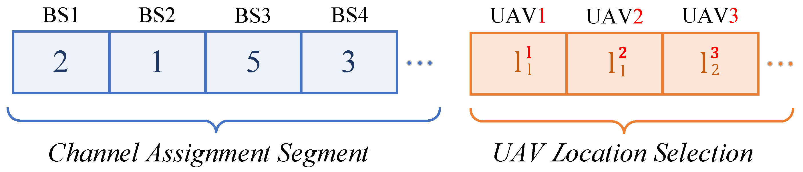
4.1. Genotypes Encoding

We first define our genotype encoding representation, i.e., the structure of each chromosome. Recall that we aim to jointly optimize UAV locations and sub-channel assignments. To do so, consider a two-part chromosome, as shown in Figure 3. The first part is called Channel Assignment Segment and is denoted by χ C , which consists of | K | genes. To elaborate, let χ C [ k ] be the k-th gene in χ C and represents a sub-channel selected for a particular cell k in set K , meaning that the first | K | genes represent a combination of all sub-channels s S .
The second part, termed UAV Location Selection Segment, is denoted by χ L . It comprises | V | genes. Let χ L [ v ] L v denote the v-th gene in χ L , representing the location selected for UAV v operating within the coverage area of its associated cell k. In addition, let collection X be a population over each generation of | X | chromosomes in total.
Figure 3 illustrates an example chromosome χ . It incorporates four base stations (cells) and three UAVs. In terms of channel assignment, represented by χ C , cells indexed by k = 1 , 2 , 3 are allocated a particular sub-band s = 2 , 1 , 5 , 3 , respectively. As for the UAV location segment, indicated by χ L , it specifies that each UAV indexed by v = 1 , 2 , 3 is assigned a position l 1 1 , l 2 1 , or  l 2 3 , respectively.

4.2. Fitness Evaluation

Each chromosome is evaluated by a fitness function to determine its quality. Let S ( χ ) = { l n ( v ) , x s ( k ) | k K , v V } be the collection of the selected location l n ( v ) L v for each UAV v, as well as the designated sub-band x s ( k ) S for each cell k represented by chromosome χ . We consider that the fitness score of a chromosome is directly proportional to its resultant fairness-aware sum-rate R for both UE and UAVs, given by a predetermined power allocation configuration for BSs. Formally, the fitness function is given by
f ( χ ) = m i n { β 1 R U A V , β 2 R U E [ 1 ] , β 2 R U E [ 2 ] } .
Here, R U A V , R U E [ 1 ] , and  R U E [ 2 ] are computed based on the sub-band assignment and UAV location decision encoded by chromosome χ . To do so, the decision variable of the transmit power, i.e.,  p k t and P v , are fixed to a predefined constant value and substituted into Equations (10)–(19):
p k t = | U k | k = 1 | K | | U k | α t P m a x , t = 1 , 2 , k K ,
P v = γ p k t , v V k .
In other words, Equation (27) specifies that the transmit power p k t of base station k is allocated proportionally to the number of UE it serves relative to the total number of UE. In Equation (28), the transmit power of UAV v is determined as a fraction of the transmit power allocated to its associated base station or cell k, i.e., regulated by γ [ 0 , 1 ] .

4.3. Selection

The roulette-wheel method [32] is used to select chromosomes based on their fitness score within a population. Specifically, the probability of selecting a specific chromosome χ from the current population X is as follows:
p ( χ ) = f ( χ ) χ X f ( χ ) .
Given by the probability distribution { P = p ( χ 1 ) , p ( χ 2 ) , , p ( χ | X | ) } , our GA retains a fraction of 5% of the best-performing chromosomes/elitist in X, stored in collection X e l i , to be directly used unchanged into the next generation. It then samples other chromosomes from the population X according to probability distribution P and stores them in collection X s a m p l e . Both collection X e l i and X s a m p l e together form a candidate parent pool for generating new chromosomes via crossover and mutation.

4.4. Crossover

We implemented a crossover operation given by the parent pool X e l i and X s a m p l e . To generate a new chromosome/offspring χ n e w , GA randomly sampled a pair of parents from the abovementioned pool, namely χ i and χ j . As we considered a two-part chromosome combining UAV location selection and sub-band assignment, our GA algorithm conducted crossover separately on each segment.
We employed uniform crossover for χ C and χ L segment, respectively. Specifically, uniform crossover ensures that each gene of offspring χ n e w is independently selected from one of its parent chromosomes, χ i or χ j . To this end, let M a s k ( χ C ) and M a s k ( χ L ) represent a randomly generated binary mask vector that is equal to the size of the χ C and χ L segments, respectively. Mathematically, a uniform crossover to generate offspring χ n e w is as follows:
χ n e w C = χ i C M a s k ( χ C ) + χ j C M a s k ( χ C ) ,
χ n e w L = χ i L M a s k ( χ L ) + χ j L M a s k ( χ L ) ,
where ⊙ represents the Hadamard product. Let collection X c r o s s store | X | | X e l i | new chromosomes.

4.5. Mutation

To avoid local optima, we employed random resetting mutation. That is, for each individual gene over offspring χ n e w in X c r o s s , with a low chance ranging from 1% to 5%, GA will reassign it a new value drawn uniformly from its solution space. To elaborate, for each gene in the χ C segment, it has a chance to be reassigned a new sub-band from s in S ; for each gene in the χ L segment corresponding to UAV v, GA may reassign it a possible location l n v in L v . After mutation, the updated offspring are stored in collection X m u t .

4.6. Population Update

The collection of elitist in X e l i and newly generated offspring in X m u t together constitute the population for the next generation. In addition, it has a generation size of | A | , whereas a chromosome χ * that exhibits the highest fitness value in the | A | -th generation is then selected for use in problem (P2).
Given by χ * , problem (P2) is now formulated as the following linear program (LP):
maximize       D p k t , z ( l n v , u ) subject   to     ( 7 ) , ( 10 ) ( 14 ) .

4.7. Discussion

We now discuss the convergence properties of our GA-based solution. According to previous work [33], a genetic algorithm is guaranteed to converge to the global optimum with a probability of one as the number of generations approaches infinity, if the following conditions are satisfied: (i) the chromosome space is finite, (ii) each gene within a chromosome has a non-zero probability of mutation, and (iii) the fittest chromosome in each generation is preserved and carried over to the next generation. The convergence proof is based on a Markov chain model, as detailed in [33]. One can easily find that our implementation satisfies all these conditions. Specifically, the total number of possible chromosomes is bounded by | S | | K | × | L | | V | , where S , K , and  L are given by (P1). In addition, we retain the top 5% of chromosomes/elitism in each generation and apply a mutation rate of at least 1%.
Indeed, numerous meta-heuristic methods can be adopted to our problem (P3). We adopted a GA-based approach due to its inherent suitability for encoding discrete variables, such as sub-channel allocation and UAV location selection, into chromosomes. Further, we chose GA because empirical studies have demonstrated its superior solution quality in discrete and combinatorial optimization tasks [34]. A comparison with other meta-heuristics is beyond the scope of this work.

4.8. Computational Complexity Analysis

We now compute the computational complexity of our GA-based solution.
Proposition 1. 
A GA-based solution has a time complexity of O ( | A | | X | ( | K | ( | U | + | V | + 1 ) + | V | ) + ϵ ) .
Proof. 
We first compute the resources used per generation. For each generation, the selection, uniform-crossover, and random-resetting mutation operators act on all | X | chromosomes, where parameter | X | is the population size. As each chromosome has | K | + | V | genes, these operators together require time complexity O ( | X | ( | V | + | K | ) per generation. For the fitness evaluation operator, first note that evaluating the fitness of a single chromosome requires computing the SINR or data rate for each UAV and UE across all cells. This has a time complexity of O ( ( | V | + | U | ) | K | ) per chromosome. This also means GA has computational complexity O ( | X | ( | V | + | U | ) | K | ) per generation. Considering | A | generations in total, this results in O ( | A | | X | ( | V | + | K | ) + ( | A | | X | ( | V | + | U | ) | K | ) ) = O ( | A | | X | ( | K | ( | U | + | V | + 1 ) + | V | ) ) .
Once the GA returns the optimal chromosome χ * , solving LP (P3) takes time O ( ϵ ) , where ϵ depends on the LP solver. For example, the interior-point method has the time complexity O ( ϵ ) = O ( n 3 / l o g ( n ) )  [35], where constant n is determined by the number of variables and constraints in LP (P3). As a result, our GA-based algorithm in total has the computational complexity O ( | A | | X | ( | K | ( | U | + | V | + 1 ) + | V | ) + ϵ ) . This completes our proof.    □

5. Results

We conducted our experiments using Python 3.11, on an Intel i7 CPU @2.90 GHz with 32 GB of memory. We solved problem (P3) using Gurobi 10.0.1. Each BS provided circular coverage with a radius between 10 and 50 meters. Moreover, they were densely deployed, whereas the coverage areas of neighboring BSs were contiguous but non-overlapping. UE and candidate UAV locations were randomly distributed within the coverage area of their associated BSs. Table 1 lists other parameters used in our evaluation.
We analyzed our problem and GA-assisted two-stage approach against the following benchmarks:
  • BF * (brute-force search): It generates exhaustive combinations of both the cell channel assignment and UAV location selection solutions. It then solves each of them using LP (P3) to determine the optimal solution. Note that BF can only be used for small-scale networks.
  • GA * : It follows the same GA procedure as described in Section 4. However, it solves problem (P2) and uses the resulting objective value as the fitness for a given chromosome. Note that there is a trade-off between computational efficiency and optimality because GA * is required to solve problem (P3) for each chromosome in one population and over all generations.
  • GA−Rand: It adopts a standard GA-based approach as outlined in [36] to manage interference levels at UE in dense wireless networks. Briefly, it solves a sub-band allocation problem with the objective of maximizing the minimum SINR among all UE. Since the originally proposed method is not directly applicable to UAV-assisted networks, we extend it by randomly selecting a candidate location for each UAV.
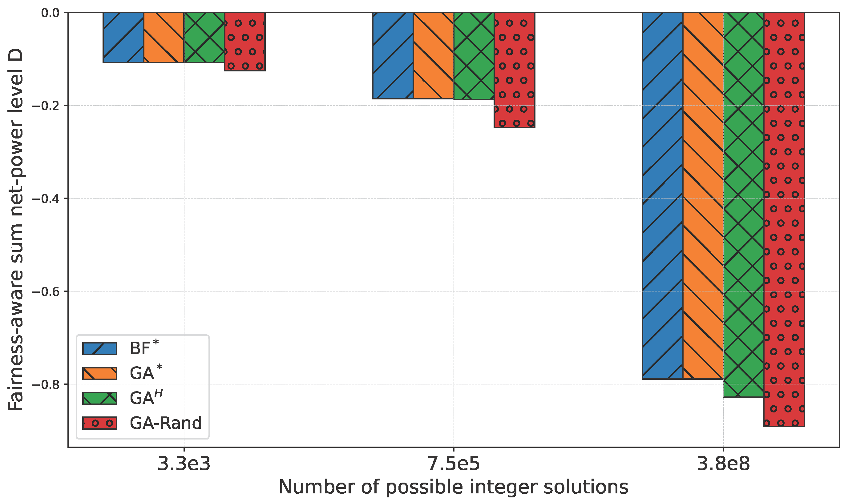
Here, we refer to our proposed solution in Section 4 as GA H . We studied our problem using GA H , GA * , and GA−Rand under the following factors: (i) the number of BSs, (ii) the number of UE, (iii) the coverage of cells, and (iv) the number of candidate UAV locations. For each simulation, we evaluated the following rate metrics: (a) fairness-aware sum-rate R in (P1), (b) fairness-aware net-power level D in (P2), and (c) the sum-rate of all UE and UAVs, calculated as S + = β 1 R U A V + β 1 R U E [ 1 ] + β 2 R U E 0 [ 2 ] + β 2 R U E V [ 2 ] . The results were obtained over an average of 50 simulation runs.

5.1. Optimality Gap

We first validate the optimality gap between BFS and GA H , and GA * and GA−Rand. We consider the following network scenarios: (i) scenario-1, where we set | K | = 3 , | S | = 3 , | V k | = 1 and | L v | = 5 , which results in a total of | S | | K | × | L v | | V | | K | = 3.3 × 10 3 possible integer solutions; (ii) scenario-2, where we set | K | = 5 , | S | = 3 , | V k | = 1 and | L v | = 5 , resulting in | S | | K | × | L v | | V | | K | = 7.5 × 10 5 ; and (iii) scenario-3, which considers | K | = 6 , | S | = 3 , | V k | = 2 and | L v | = 3 , yielding 3.8 × 10 8 possible integer solutions for each run.
Referring to Figure 4, for scenario-1, observe that both GA * and GA H achieve 99.99% of the optimal solution with respect to the sum net-power level D. For scenario-2, the optimality gap between GA H and BF * slightly increases by 0.75%. This is expected given that the search space of problem (P3) in scenario-2 is over 200 times larger than that in scenario-1. For the same reason, the optimality gap between GA H continues to increase by 4.4% in scenario-3. This shows that an exponential increase in the problem complexity causes only a marginal degradation of GA H in small-scale networks. Also, note that GA * achieves 99.99% of the optimal solution across all scenarios.
Figure 5 compares their computation time. The brute-force search ( BF * ) requires 4.5, 1.33 × 10 3 , and 1.17 × 10 6 seconds for scenario-1, scenario-2, and scenario-3, respectively. The computation time for GA * increases from 18.68 to 91.9 seconds as the problem complexity grows. Note that G A * requires more computation time than brute-force search in scenario-1. This is because it solves LP (P3) with 2 × 10 4 times, which far exceeds the total number of 3.3 × 10 3 possible integer solutions. Furthermore, GA H solves the problems in 3.90, 8.53, and 29.02 seconds for scenario-1, scenario-2, and scenario-3, respectively. This means the computational efficiency of GA H is approximately 4.6 orders of magnitude lower than that of the brute-force search in small-scale networks.

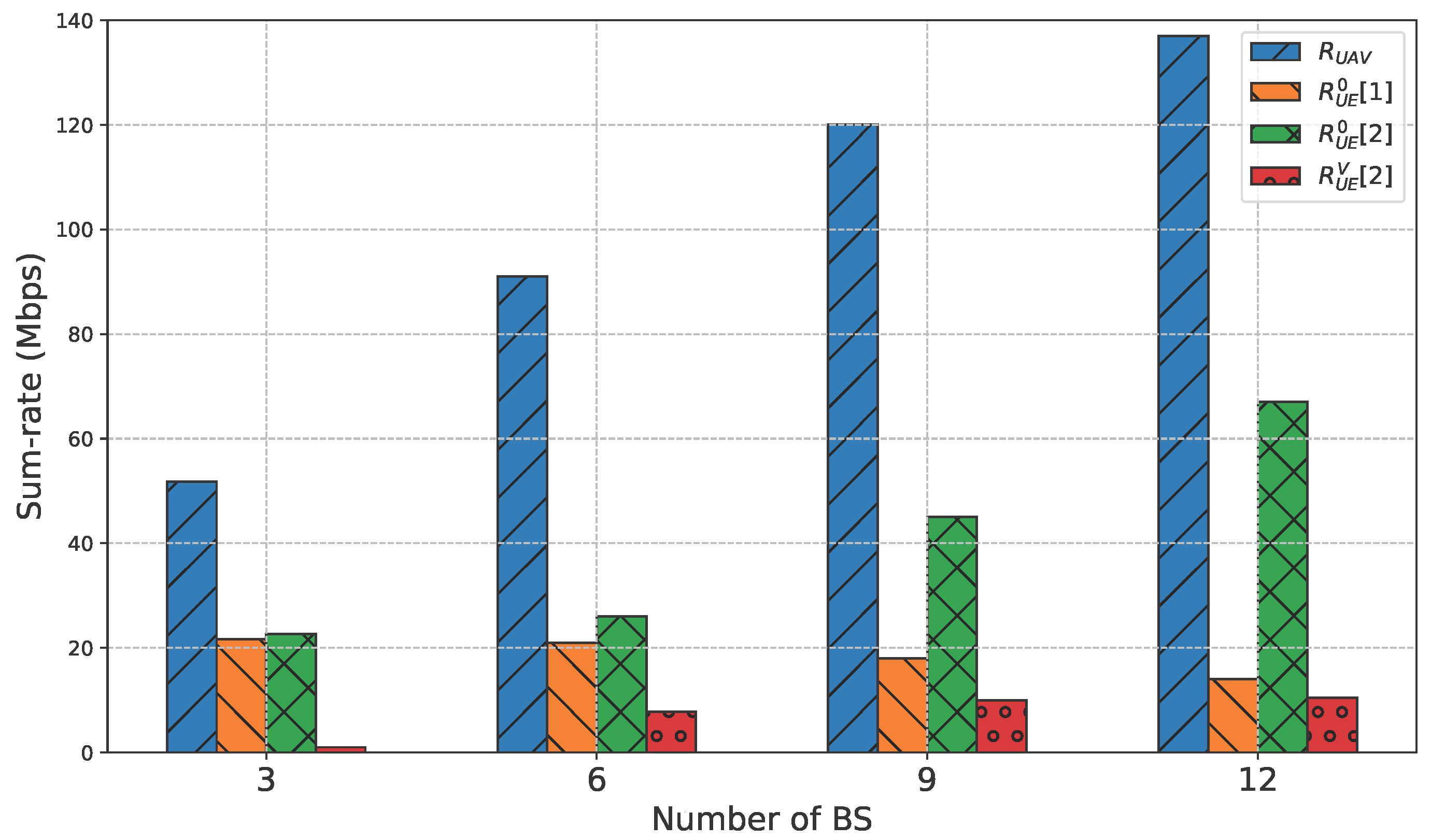
5.2. Number of Base Stations

Here, we fix the number of available sub-bands to | S | = 6 . Each BS k directly serves a set of | U 0 k | = 5 UE. In addition, there are | V | = 10 UAVs in total available for all BSs. We assign UAVs to BSs in a round-robin fashion. Furthermore, each UAV v has a candidate location set with size | L v | = 20 .
Referring to Figure 6a, the sum-rate S + computed by GA H increases from 101.94 to 227.28 (in Mbps) as the number of BS increases from 3 to 12. The sum-rate S + computed by GA * increases from 97 to 228.8 (in Mbps), and that of GA−Rand increases from 76 to 210 (in Mbps). This is because additional BSs will support more UE, thereby improving sum-rate R U E 0 [ 1 ] and R U E 0 [ 2 ] . Note that GA * and GA H outperform GA−Rand with respect to R and S + . This is expected as GA−Rand does not optimize UAV placement to mitigate the interference between UAVs and UE.
Observe that in Figure 6b,c, the fairness-aware sum-rate R and sum net-power level D computed by GA H increases from 1.2 to 10.88 (in Mbps), and increases from −0.15 to −0.08 (in Watt), respectively. For GA * and GA−Rand, their computed R increases from 1.53 to 10.86 (in Mbps), and from 0.194 to 4.94 (in Mbps), respectively.
To explain the increase in metric R and D, we examine the minimum value among the following components of sum-rate S + : { β 1 R U A V , β 1 R U E [ 1 ] , β 2 R U E 0 [ 2 ] , β 2 R U E V [ 2 ] } , as shown in Figure 7. It considers scenarios with | K | = 3, 6, 9, and 12. Observe that the sum-rate of the data links from UAVs to UE, i.e., R U E V [ 2 ] , reaches the minimum value. This can be attributed to the following main reasons. First, the distance between UAVs and UE is significantly larger than that between BSs and UE. According to the aerial channel models in Equations (4) and (5), for the given altitudes setting in Table 1, the path loss from UAVs to UE is greater than that from BSs to UE. As a result, UAV-UE links will have lower received power and are more susceptible to environmental noise, which explains why the sum-rate of UAV-UE links is lower compared to BS-UE links. Second, BSs are the only interfering sources for BS-UAV and BS-UE links. However, UAV-UE links are subject to both inter-cell and intra-cell interferences from both BSs and neighboring UAVs operating on the same sub-band, resulting in lower SINR accordingly. This explains why the rate of UAV-UE links is lower than that of other link types.
Given these findings, the improvement in fairness-aware sum-rate R and sum net-power level D with an increasing number of BSs is because UAVs are distributed more sparsely. That is, for a fixed total number of UAVs, an increase in the number of BSs/cells results in fewer UAVs per cell. This allows UAVs to be placed further from UE served by the other UAVs, thereby reducing both inter-cell and intra-cell interferences on the UAV-UE links. This consequently increases R U E V [ 2 ] , which in turn increases both R and D.

5.3. Coverage per Cell

Here, we deploy ten BSs/cells and vary their coverage radius from 20 to 60 meters in increments of 10 meters. We set | K | = 6 , | V | = 8 , and | S | = 4 .
As shown in Figure 8, the sum-rate for UE and UAVs computed by GA H decreases from 264 to 187 (in Mbps) when the coverage radius increases from 20 to 60 meters. This is because with a larger coverage area, randomly distributed UE and UAVs are more likely to establish longer communication links with the BSs. Longer BS-UE links and BS-UAV links mean higher signal attenuation, thereby lowering their SINR or rate under a constant environmental noise level accordingly.
Observe that the fairness-aware sum-rate R computed by GA H increases from 2.64 to 12.57 (in Mbps). This is because expanded cell coverage enables UAVs to be distributed more widely, both from one another or from BSs in other cells. This helps reduce both intra-cell and inter-cell interferences, thereby increasing the minimum data rate for UE and UAVs.

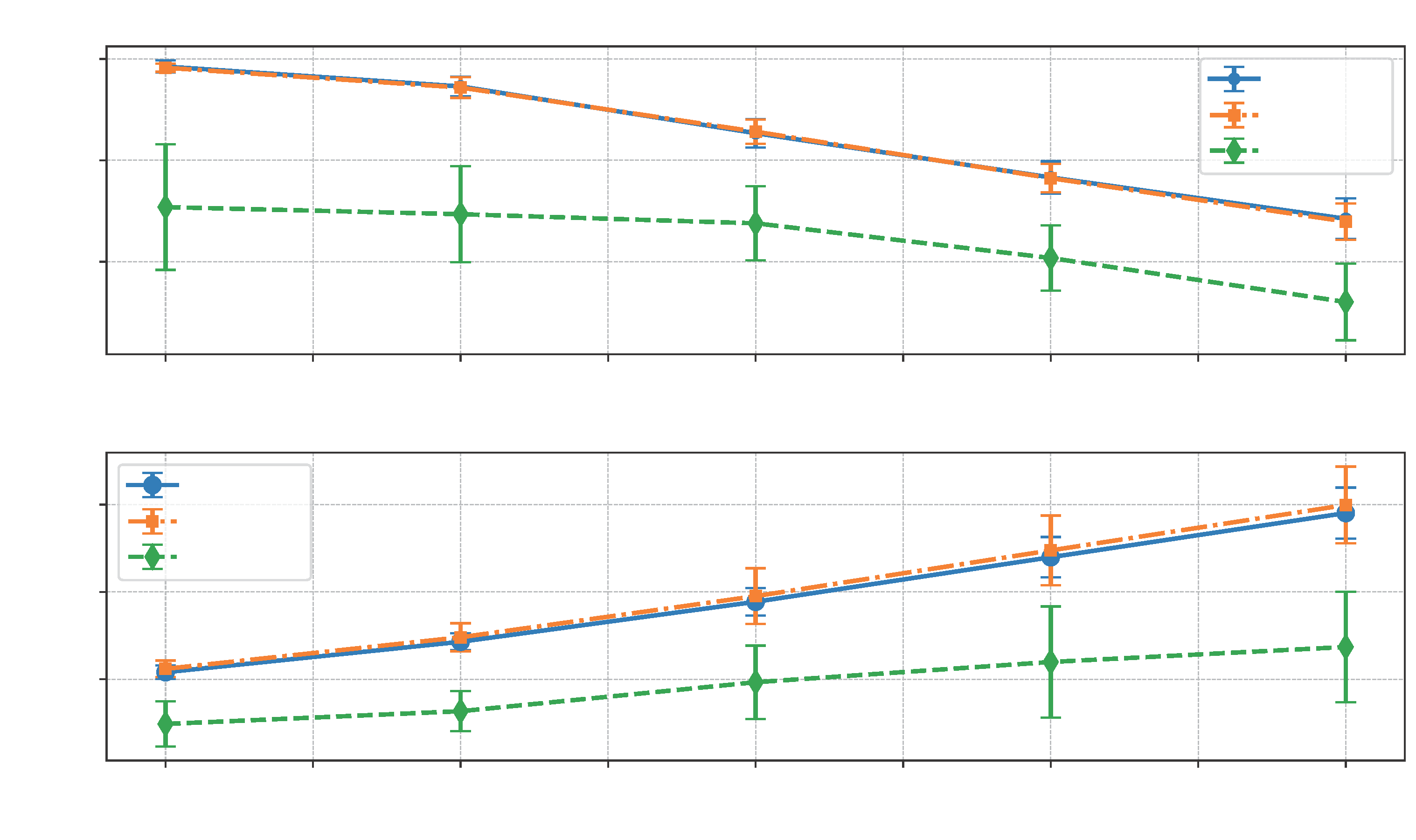
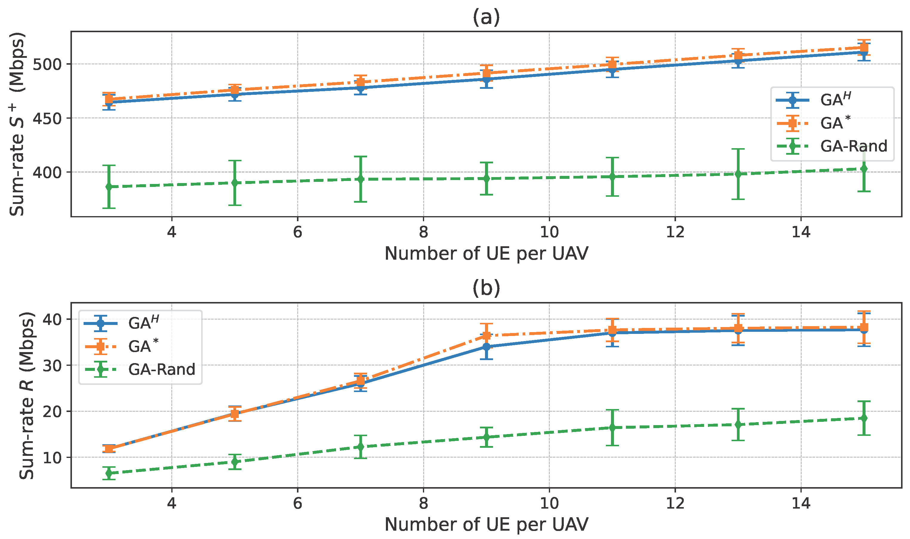
5.4. Number of UE per Cell

We consider ten BSs and ten UAVs. Each cell has a coverage of 30 meters. Each BS serves five UE directly. The number of sub-bands is fixed at | S | = 4 .
Figure 9 shows that both the sum-rate S + and the fairness-aware sum-rate R increase as the number of UE associated with each UAV grows. This is expected due to the increasing number of active downlinks. However, the fairness-aware sum-rate R does not significantly improve after | U v k | reaches 11. This is because at small values of | U v k | , the sum-rate β 2 R U E V [ 2 ] restricts the minimum sum-rate of all transmissions due to the limited number of active UAV-UE links. As the number of UE associated with UAVs increases, the number of UAV-UE links becomes over 100 times greater than that of BS-UAV links. Consequently, the sum-rate of UAV-UE links exceeds that of BS-UAV links, i.e., R U E V [ 2 ] > R U A V . That is, since the sum-rate of UAV-UE links is no longer the minimum of the set { β 1 R U A V , β 1 R U E [ 1 ] , β 2 R U E 0 [ 2 ] , β 2 R U E V [ 2 ] } , further increases in | U v k | will not help to improve the fairness-aware sum-rate R. Note that since GA−Rand only optimizes the sub-band allocation for cells without considering the location of UAVs based on the location of BSs and UE, it provides the least improvement in both the sum-rate S + and the fairness-aware sum-rate R. The optimality gap between GA H and GA−Rand becomes larger as each UAV serves more UE.

6. Conclusions

This article has studied the problem of joint sub-carrier transmit power allocation and UAV placement in OFDMA-based multi-cell networks. The goal is to maximize the fairness-aware sum-rate of all UE and UAVs. The problem is solved via a two-layer approach. The results show that the proposed two-stage approach achieves approximately 97.43% of the optimal fairness-aware sum-rate obtained via brute-force search in small-scale networks. It also outperforms a competitive GA-based sub-band allocation heuristic with respect to the sum-rate at UE and UAVs and the aforementioned fairness-aware sum-rate by 126.72% and 221.39%, respectively.
There are a number of promising future directions. One direction is to account for time-varying or random channel state information. In this aspect, data-driven approaches such as reinforcement learning (RL) and deep learning (DL) can be employed to optimize both sub-band allocation and UAV placement. Another potential improvement is to jointly optimize UE assignment to UAVs and cells in addition to the problem at hand, which is expected to yield higher sum-rate and fairness. Another future direction is to incorporate multi-antenna techniques to enhance capacity and better manage interference.
Apart from that, issues such as UAV energy consumption and route planning, to name a few, can impact long-term system and solution performance, e.g., in multiple-time-slot cases. For example, UAVs are typically battery-powered and have limited flight endurance, which may require them to periodically return to charging stations or base locations for recharging. They may also need to relocate across different areas to accommodate dynamic user demands. Therefore, optimizing UAV positions over successive time slots should take into account residual energy levels and flight speed constraints, as UAVs cannot be repositioned arbitrarily or instantaneously in practice. From this perspective, UAV route or trajectory planning represents a promising research direction, as it can simultaneously improve energy efficiency and enhance QoS metrics in multi-cell networks.

Author Contributions

Conceptualization, M.J. and H.R.; writing—original draft preparation, M.J. and H.R.; writing—review and editing, M.J., H.R. and T.W.; supervision, Y.Q. and T.W.; software, M.J. All authors have read and agreed to the published version of the manuscript.

Funding

This research was funded by the Key Research Project of Zhejiang Province, China, under No. 2025C01083.

Institutional Review Board Statement

Not applicable.

Informed Consent Statement

Not applicable.

Data Availability Statement

The original contributions presented in this study are included in the article. One can request from the corresponding author for further inquiries.

Conflicts of Interest

The authors declare no conflicts of interest.

References

  1. Tinh, B.T.; Nguyen, L.D.; Kha, H.H.; Duong, T.Q. Practical Optimization and Game Theory for 6G Ultra-Dense Networks: Overview and Research Challenges. IEEE Access 2022, 10, 13311–13328. [Google Scholar] [CrossRef]
  2. Khorov, E.; Kiryanov, A.; Lyakhov, A.; Bianchi, G. A Tutorial on IEEE 802.11ax High Efficiency WLANs. IEEE Commun. Surv. Tuts. 2019, 21, 197–216. [Google Scholar] [CrossRef]
  3. López Raventós, Á.; Bellalta, B. Concurrent decentralized channel allocation and access point selection using multi-armed bandits in multi BSS WLANs. Elsevier Comput. Netw. 2020, 180, 107381. [Google Scholar] [CrossRef]
  4. Gao, H.; Feng, J.; Xiao, Y.; Zhang, B.; Wang, W. A UAV-Assisted Multi-Task Allocation Method for Mobile Crowd Sensing. IEEE Trans. Mob. Comput. 2023, 22, 3790–3804. [Google Scholar] [CrossRef]
  5. Wu, K.; Chin, K.W.; Soh, S. Multi-UAVs Network Design Algorithms for Computed Rate Maximization. IEEE Trans. Mob. Comput. 2024, 23, 8965–8980. [Google Scholar] [CrossRef]
  6. Song, Z.; Chin, K.W.; Yang, C.; Ros, M. Methods to Assign UAVs for K-Coverage and Recharging in IoT Networks. IEEE Trans. Mob. Comput. 2024, 23, 2504–2519. [Google Scholar] [CrossRef]
  7. Forghani, A.; Chin, K.W.; Ros, M. Scheduling Services in Multi-UAVs IoT Networks. IEEE Internet Things J. 2025; Early Access. [Google Scholar] [CrossRef]
  8. Forghani, A.; Chin, K.W.; Ros, M. Optimizing Virtual Functions Deployment in Multi-UAV IoT Networks. IEEE Internet Things J. 2024, 11, 20367–20378. [Google Scholar] [CrossRef]
  9. Cui, Y.; Chin, K.W.; Soh, S. Maximizing UAV Tasks Computation Quality in Energy Harvesting IIoT. IEEE Trans. Ind. Inform. 2025, 21, 4447–4456. [Google Scholar] [CrossRef]
  10. Kim, J.; Park, S.; Jung, S.; Cordeiro, C. Cooperative Multi-UAV Positioning for Aerial Internet Service Management: A Multi-Agent Deep Reinforcement Learning Approach. IEEE Trans. Netw. Serv. Manag. 2024, 21, 3797–3812. [Google Scholar] [CrossRef]
  11. Hamza, A.S.; Khalifa, S.S.; Hamza, H.S.; Elsayed, K. A survey on inter-cell interference coordination techniques in OFDMA-based cellular networks. IEEE Commun. Surv. Tuts 2013, 15, 1642–1670. [Google Scholar] [CrossRef]
  12. Kosta, C.; Hunt, B.; Quddus, A.U.; Tafazolli, R. On interference avoidance through inter-cell interference coordination (ICIC) based on OFDMA mobile systems. IEEE Commun. Surv. Tuts 2012, 15, 973–995. [Google Scholar] [CrossRef]
  13. Chiecochan, S.; Hossain, E.; Diamond, J. Channel Assignment Schemes for Infrastructure-Based 802.11 WLANs: A Survey. IEEE Commun. Surv. Tuts 2010, 12, 124–136. [Google Scholar] [CrossRef]
  14. Nakashima, K.; Kamiya, S.; Ohtsu, K.; Yamamoto, K.; Nishio, T.; Morikura, M. Deep Reinforcement Learning-Based Channel Allocation for Wireless LANs With Graph Convolutional Networks. IEEE Access 2020, 8, 31823–31834. [Google Scholar] [CrossRef]
  15. Oh, H.; Jeong, D.G.; Jeon, W.S. Joint Radio Resource Management of Channel-Assignment and User-Association for Load Balancing in Dense WLAN Environment. IEEE Access 2020, 8, 69615–69628. [Google Scholar] [CrossRef]
  16. Luo, Y.; Chin, K.W. Learning to bond in dense WLANs with random traffic demands. IEEE Trans. Vehic. Tech. 2020, 69, 11868–11879. [Google Scholar] [CrossRef]
  17. Sarwar, M.Z.; Chin, K.W. On Supporting Legacy and RF Energy Harvesting Devices in Two-Tier OFDMA Heterogeneous Networks. IEEE Access 2018, 6, 62538–62551. [Google Scholar] [CrossRef]
  18. Chih, T.H.; Su, S.L.; Hung, T.M. Two-phase downlink subcarrier allocation for multicell OFDMA systems. Springer Wirel. Networks 2018, 25, 2081–2090. [Google Scholar] [CrossRef]
  19. Mei, W.; Wu, Q.; Zhang, R. Cellular-Connected UAV: Uplink Association, Power Control and Interference Coordination. IEEE Trans. Wirel. Commun. 2019, 18, 5380–5393. [Google Scholar] [CrossRef]
  20. Challita, U.; Saad, W.; Bettstetter, C. Interference Management for Cellular-Connected UAVs: A Deep Reinforcement Learning Approach. IEEE Trans. Wirel. Commun. 2019, 18, 2125–2140. [Google Scholar] [CrossRef]
  21. Mei, W.; Zhang, R. Cooperative Downlink Interference Transmission and Cancellation for Cellular-Connected UAV: A Divide-and-Conquer Approach. IEEE Trans. Wirel. Commun. 2020, 68, 1297–1311. [Google Scholar] [CrossRef]
  22. Nguyen, M.D.; Ho, T.M.; Le, L.B.; Girard, A. UAV Trajectory and Sub-channel Assignment for UAV Based Wireless Networks. In Proceedings of the IEEE WCNC, Virtual Conference, Seoul, Republic of Korea, 25–28 May 2020; pp. 1–6. [Google Scholar]
  23. He, Y.; Wang, D.; Huang, F.; Zhang, R.; Pan, J. Trajectory Optimization and Channel Allocation for Delay Sensitive Secure Transmission in UAV-Relayed VANETs. IEEE Trans. Veh. Technol. 2022, 71, 4512–4517. [Google Scholar] [CrossRef]
  24. Zhai, D.; Li, H.; Tang, X.; Zhang, R.; Ding, Z.; Yu, F.R. Height Optimization and Resource Allocation for NOMA Enhanced UAV-Aided Relay Networks. IEEE Trans. Commun 2021, 69, 962–975. [Google Scholar] [CrossRef]
  25. Liu, X.; Lai, B.; Gou, L.; Lin, C.; Zhou, M. Joint Resource Optimization for UAV-Enabled Multichannel Internet of Things Based on Intelligent Fog Computing. IEEE Trans. Netw. Sci. Eng. 2021, 8, 2814–2824. [Google Scholar] [CrossRef]
  26. Singh, S.; Kumbhar, A.; Guvenc, I.; Sichitiu, M.L. Distributed Approaches for Inter-Cell Interference Coordination in UAV-Based LTE-Advanced HetNets. In Proceedings of the IEEE 88th VTC, Chicago, IL, USA, 27–30 August 2018; pp. 1–6. [Google Scholar]
  27. Ahmad, I.; Hussain, S.; Mahmood, S.N.; Mostafa, H.; Alkhayyat, A.; Marey, M.; Abbas, A.H.; Abdulateef Rashed, Z. Co-Channel Interference Management for Heterogeneous Networks Using Deep Learning Approach. Information 2023, 14, 139. [Google Scholar] [CrossRef]
  28. Lopez-Perez, D.; Guvenc, I.; De la Roche, G.; Kountouris, M.; Quek, T.Q.; Zhang, J. Enhanced intercell interference coordination challenges in heterogeneous networks. IEEE Wirel. Commun. 2011, 18, 22–30. [Google Scholar] [CrossRef]
  29. Study on Channel Model for Frequencies from 0.5 to 100 Ghz. 2022. Available online: https://www.etsi.org/deliver/etsi_tr/138900_138999/138901/16.01.00_60/tr_138901v160100p.pdf (accessed on 22 December 2024).
  30. Study on Enhanced LTE Support for Aerial Vehicles. 2017. Available online: https://www.tech-invite.com/3m36/tinv-3gpp-36-777.html (accessed on 22 December 2024).
  31. Wang, Z. A survey on convex optimization for guidance and control of vehicular systems. Annu. Rev. Control 2024, 57, 100957. [Google Scholar] [CrossRef]
  32. Lipowski, A.; Lipowska, D. Roulette-wheel selection via stochastic acceptance. Phys. A Stat. Mech. Its Appl. 2012, 391, 2193–2196. [Google Scholar] [CrossRef]
  33. Bhandari, D.; Murthy, C.A.; Pal, S.K. Genetic Algorithm with Elistist Model and Its Convergence. Int. J. Pattern Recognit. Artif. Intell. 1996, 10, 731–747. [Google Scholar] [CrossRef]
  34. Hassan, R.; Cohanim, B.; de Weck, O.; Venter, G. A Comparison of Particle Swarm Optimization and the Genetic Algorithm. In Proceedings of the 46th AIAA/ASME/ASCE/AHS/ASC Structures, Structural Dynamics and Materials Conference, Austin, TX, USA, 18–21 April 2005. [Google Scholar]
  35. Potra, F.A.; Wright, S.J. Interior-point methods. J. Comput. Appl. Math. 2000, 124, 281–302. [Google Scholar] [CrossRef]
  36. Hu, X.; Ge, S.; Xiao, J. Channel allocation based on genetic algorithm for multiple IEEE 802.15.4-compliant wireless sensor networks. In Proceedings of the ICSPCC, Xiamen, China, 22–25 October 2017. [Google Scholar]
Figure 1. An example multi-cell network with UE and cellular-assisted UAVs. Solid arrows denote a transmission over a given sub-band (color). Dotted arrows show interference from nearby cells assigned the same sub-band.
Information 16 00481 g001
Figure 2. Flowchart of the GA-based two-stage approach. In Stage-1, the GA optimizes UAV placement and BS sub-band selection. In Stage-2, using the chromosome χ * with the highest fitness, it then solves problem (P3) to determine the optimal transmit power for each BS and UAV.
Information 16 00481 g002
Figure 3. Example of a two-part chromosome.
Information 16 00481 g003
Figure 4. Optimality gap between the brute-force, GA H , GA * and GA−Rand.
Information 16 00481 g004
Figure 5. Comparison of computation time of the brute-force, GA H , GA * and GA−Rand. Note the log scale.
Information 16 00481 g005
Figure 6. Impact of the number of BSs on (a) sum-rate S + , (b) fairness-aware sum-rate R, and (c) fairness-aware sum net-power level D.
Information 16 00481 g006
Figure 7. The sum-rate of β 1 R U A V , β 1 R U E [ 1 ] , β 2 R U E 0 [ 2 ] , β 2 R U E V [ 2 ] when | K | is 3, 6, 9, and 12, respectively.
Information 16 00481 g007
Figure 8. Impact of cell coverage on (a) the sum-rate S + at UE and UAVs, and (b) the fairness-aware sum-rate R (in Mbps).
Information 16 00481 g008
Figure 9. Impact of the number of UE served by each UAV on (a) the sum-rate S + , and (b) the fairness-aware sum-rate R (in Mbps).
Information 16 00481 g009
Table 1. Simulation parameters.
ParameterValue(s)ParameterValue(s)
K5–20BS coverage20–60 m
B1 MHz | S | 4–6
P m a x 5 W σ 2 90 dBm/Hz
| U 0 k | 2–10 | U v k | 2–5
L v 5–20 | X | 100
f c 2 GHz | A | 200
h u 1.5 m h 0 25
h n v 100–300 β 0.5
Disclaimer/Publisher’s Note: The statements, opinions and data contained in all publications are solely those of the individual author(s) and contributor(s) and not of MDPI and/or the editor(s). MDPI and/or the editor(s) disclaim responsibility for any injury to people or property resulting from any ideas, methods, instructions or products referred to in the content.

