Application of a KAN-LSTM Fusion Model for Stress Prediction in Large-Diameter Pipelines

Abstract

Accurately predicting stress in large-diameter sewage pipelines is critical for ensuring their structural reliability and safety. To meet the safety requirements of large-diameter concrete pipes, we propose a hybrid model that integrates Kolmogorov-Arnold Networks (KAN) with Long Short-Term Memory (LSTM) neural networks. The model is trained and validated using actual pipeline monitoring data, ensuring that it accurately captures both the temporal dependencies and nonlinear stress patterns inherent in such systems. By modifying the fully connected layer of the original LSTM model, we develop a novel LSTM-KAN model and evaluate its performance through comprehensive predictive analysis. Comparisons with a traditional LSTM model reveal that the LSTM-KAN model—in which the fully connected layer is replaced by a KAN layer—achieves significantly lower loss and higher accuracy with fewer training iterations. Specifically, the proposed model attains a mean absolute error (MAE) of 0.033, a root mean square error (RMSE) of 0.035, and a coefficient of determination (R²) of 0.92, underscoring its superior accuracy and efficiency, and it can be used for the long-term prediction of stress in large-diameter pipes. Moreover, the integration of KAN significantly improves the nonlinear modeling capacity of the conventional LSTM, enabling the hybrid model to effectively capture complex stress variations under variable operating conditions. This work not only provides novel technical support for the application of deep learning in pipeline stress prediction but also offers a robust framework adaptable to other structural health monitoring applications.

1. Introduction

With the rapid development of China’s economy and continuous improvement of living standards, the demand for and scale of sewage pipelines has expanded significantly. However, this necessary expansion has introduced a range of challenges, particularly regarding the long-term operational integrity and safety of these critical infrastructure components. In the later stages of operation, underground sewage pipelines are subject to stress variations caused by varying external soil loads, soil deformation around the pipes, temperature gradients, and seismic activity [1]. Such variations can result in uneven ground settlement, pipeline deformation, joint failures, and ultimately, sewage leakage, all of which pose serious threats to public health and the environment [2].

Moreover, although underground sewage pipe networks are equipped with manholes positioned in accordance with municipal engineering codes to facilitate routine inspection, desilting, and maintenance, their deep burial and constant exposure to inundated and corrosive environments render frequent on-site inspections and manual monitoring impractical, challenging, and costly. This inaccessibility increases long-term risks, as undetected damage may propagate and lead to catastrophic failure. Consequently, continuous and reliable monitoring of pipeline stress data is essential for proactive maintenance, failure prevention, and ensuring operational safety.

Traditional monitoring methods typically rely on physical principles to infer stress. One common approach measures strain at discrete points using strain gauges or fiber optic sensors; this data, combined with material properties (e.g., Young’s modulus, Poisson’s ratio) and Hooke’s law, is used to calculate stress [3]. Another method employs vibration analysis, where vibrational characteristics (e.g., natural frequencies, mode shapes, and damping ratios) are measured to establish a mapping between the vibration amplitude and stress, often using finite element models or empirical relationships [4]. Although these methods provide valuable insights, they suffer from significant drawbacks, including complex sensor installations and the challenge of extrapolating localized measurements along extensive pipelines.

To address these limitations, several studies have explored alternative approaches. For example, Zhang Hang [5] developed a nonlinear soil-spring model to simulate the stress distribution in pipelines under landslide conditions, offering a more realistic representation of soil-structure interaction. He Yaying [6] employed distributed optical fiber sensing for continuous, real-time stress monitoring and validated its accuracy via finite element analysis. El-ABBASY et al. [7] used an artificial neural network (ANN) to predict pipeline deterioration states based on historical inspection data, while Liu Yuqing et al. [8] derived a formula relating the axial stress measured by vibration-string sensors to the true stress state. Despite these advances, such methods often lack an in-depth analysis of long-term trends and complex patterns, limiting their ability to forecast phenomena like pipeline–soil separation, significant displacements, or critical stress levels preceding failure. Moreover, they depend on precise material properties and boundary conditions, which are difficult to obtain for aging pipelines.

Recent advances in machine learning, particularly deep learning, have introduced promising data-driven approaches that can mitigate the limitations of traditional models [9]. Since stress monitoring data are inherently time series, Long Short-Term Memory (LSTM) networks—designed to learn long-term dependencies in sequential data—are well-suited for capturing the complex temporal dynamics of pipeline stress [10]. Their effectiveness has been demonstrated in applications ranging from machine translation to DNA sequence analysis and time-series forecasting [11].

In 2021, Leng Jiancheng et al. [12] proposed a stress prediction method for pipelines under foundation settlement by combining a Backpropagation (BP) neural network with a Grey Model (GM (0,1)); however, their method tended to be conservative potentially overestimating stress levels. In 2022, Liu Xiang [13] applied an LSTM model to pipeline stress prediction for the first time, demonstrating its scientific validity and potential for early failure warning.

More recently, Liu et al. [14] introduced the Kolmogorov-Arnold Network (KAN), a novel architecture that deepens the shallow Kolmogorov network by representing multivariate functions as compositions of univariate functions with desirable approximation characteristics. Chen S et al. [15] further improved prediction accuracy by combining LSTM with ensemble learning and convolutional neural networks (CNN), illustrating the benefits of hybrid modeling. However, research combining KAN and LSTM for time series analysis remains limited in the context of pipeline stress prediction, presenting an opportunity to explore their synergistic potential. Unlike Multi-Layer Perceptrons (MLPs) that use fixed activation functions, KANs learn their activation functions during training—often employing B-spline functions for their excellent fitting capabilities and smoothness [16]. By optimizing these functions, the KAN enhances feature representation and efficient scaling, potentially yielding significant performance improvements over conventional fully connected layers in LSTM.

This study proposes and implements an innovative hybrid model, the LSTM-KAN model, which synergistically combines LSTM’s robust memory capabilities with KAN’s advanced nonlinear representation. The model leverages LSTM’s strength in capturing temporal dependencies while exploiting KAN’s ability to learn complex nonlinear relationships between input features and predicted stress. This approach overcomes the limitations of single-model strategies and offers new insights into the application of deep learning for structural health monitoring and predictive maintenance in civil infrastructure. The research objectives are as follows: (1) construct a robust LSTM-KAN hybrid framework by carefully designing the architecture and interconnections; (2) explore effective integration mechanisms between LSTM and KAN through various combination strategies; (3) validate improvements in prediction accuracy, stability, and generalization using comprehensive historical pipeline stress data, and compare the performance against standalone LSTM and KAN models as well as benchmark methods; and (4) analyze the impact of incorporating KAN on LSTM performance by examining the learned activation functions and underlying theoretical foundations. Ultimately, the goal is to develop a practical tool that enables pipeline operators to proactively assess asset conditions, anticipate potential issues, and optimize maintenance schedules—thereby enhancing the safety and longevity of these vital infrastructure systems. At the same time, the LSTM-KAN model proposed in this paper, as the core model for pipeline stress prediction, demonstrates superior accuracy compared to the pipeline stress prediction model by Liu Xiang [13], Zhou Lifeng [17] and Bian Xi’ao’yan [18] et al. mentioned earlier. The LSTM-KAN model’s pipeline stress prediction capability is a key element of the automated pipeline safety decision-making platform, signifying its gradual alignment with AI-driven industrial automation.

2. Methodology

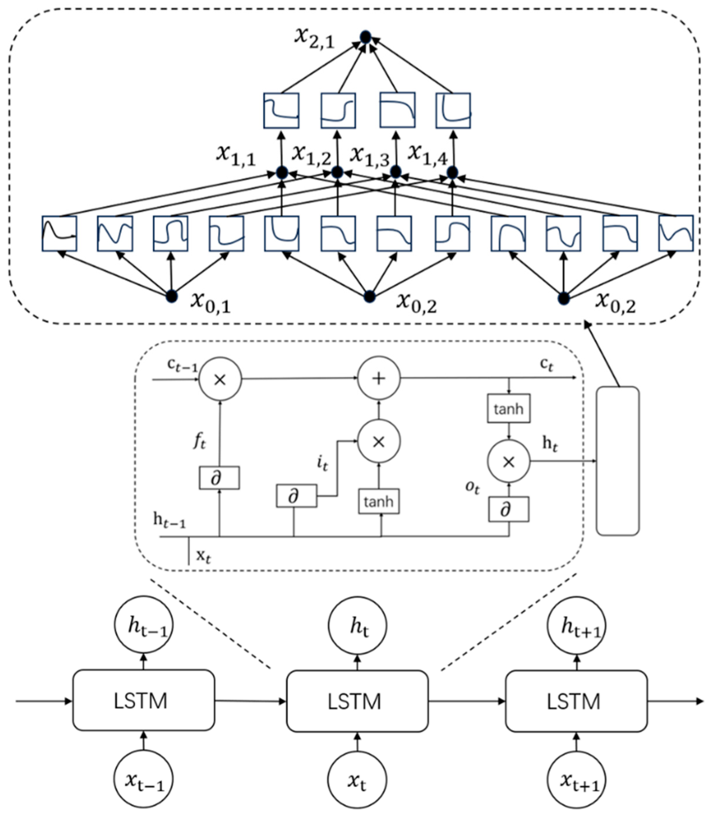
2.1. Principles of the Long Short-Term Memory (LSTM) Network Algorithm

Recurrent Neural Networks (RNNs) are models specifically designed for processing time-series data by employing backpropagation through time. This mechanism allows the network to use previous time-step states as inputs for current predictions, theoretically enabling RNNs to retain long-term contextual information through internal activation storage and thereby learn and exploit temporal dependencies. In practice, however, RNNs often encounter vanishing and exploding gradient problems that severely hinder their ability to learn long-term dependencies [19].

To address these issues, researchers have developed improved models, such as Long Short-Term Memory networks (LSTMs). LSTMs are a specialized form of RNN that incorporates gating mechanisms and a cell state design—combined with optimized parameter selection and training processes—to effectively overcome the vanishing gradient problem. Consequently, LSTMs demonstrate enhanced performance and stability when processing long sequences. Moreover, the gating mechanisms facilitate the capture and utilization of long-term dependencies by using the cell state as the primary conduit for information flow, selecting appropriate activation functions, and applying parameter optimization techniques to further mitigate the exploding gradient issue [20].

The neuronal structure of LSTM is shown in Figure 1. The core of an LSTM cell comprises three gates and a cell state:

• Forget Gate: Determines the extent to which information from the previous cell state should be discarded.

  $$f_t=\sigma (W_f\left[h_{t-1},x_t\right]+b_f)$$

  (1)
  Here $f_t$ is the forget gate, $\sigma$ denotes the sigmoid function, $W_f$ is the weight matrix for the forget gate, $b_f$ is the bias term, and $\left[h_{t-1},x_t\right]$ represents the concatenation of the previous hidden state $h_{t-1}$ and the current input $x_t$.
• Input Gate: Determines the amount of the current input that should be stored in the cell state.
  Input Gate Activation:

  $$i_t=\sigma (W_i\left[h_{t-1},x_t\right]+b_i)$$

  (2)
  Candidate Cell State:

  $${\tilde{C}}_t=tanh(W_c\left[h_{t-1},x_t\right]+b_c)$$

  (3)
  In these equations, $i_t$ is the input gate, $\tilde{C}$ is the candidate cell state, $tanh$ represents the hyperbolic tangent function, $W_i$ and $W_c$ are weight matrices and $b_i$ and $b_c$ are bias terms.
• Output Gate: Determines the amount of information from the cell state to be output to the hidden state.

  $$o_t=\sigma (W_o\left[h_{t-1},x_t\right]+b_o)$$

  (4)
  Here, $o_t$ is the output gate, $W_o$ is the weight matrix for the output gate, and $b_o$ is its bias term.
• Cell State: Preserves long-term information and propagates it along the sequence.

  $$C_t=f_t\ast C_{t-1}+i_t\ast {\tilde{C}}_t$$

  (5)
  LSTM Output:

  $$h_t=o_t\ast tanh\left(C_t\right)$$

  (6)
  In these equations, $C_t$ is the cell state at the current time, $C_{t-1}$ is the cell state at the previous time, and the symbol $\ast$ denotes element-wise multiplication.

At each time step t, the LSTM processes the current input $x_t$ along with the previous hidden state $h_{t-1}$ and cell state $c_{t-1}$. It then updates the cell state $c_t$ and hidden state $h_t$ using the forget, input, and output gates. The forget gate determines which information in $c_{t-1}$ should be retained or discarded. The input gate selects new information to incorporate into the cell state and generates a candidate value, ${\tilde{\mathrm{c}}}_{\mathrm{t}}$; subsequently, the cell state is updated by combining the outputs of the forget and input gates. Finally, the output gate decides which portions of the updated cell state $c_t$ are passed to the hidden state $h_t$ for use in subsequent layers or time steps.

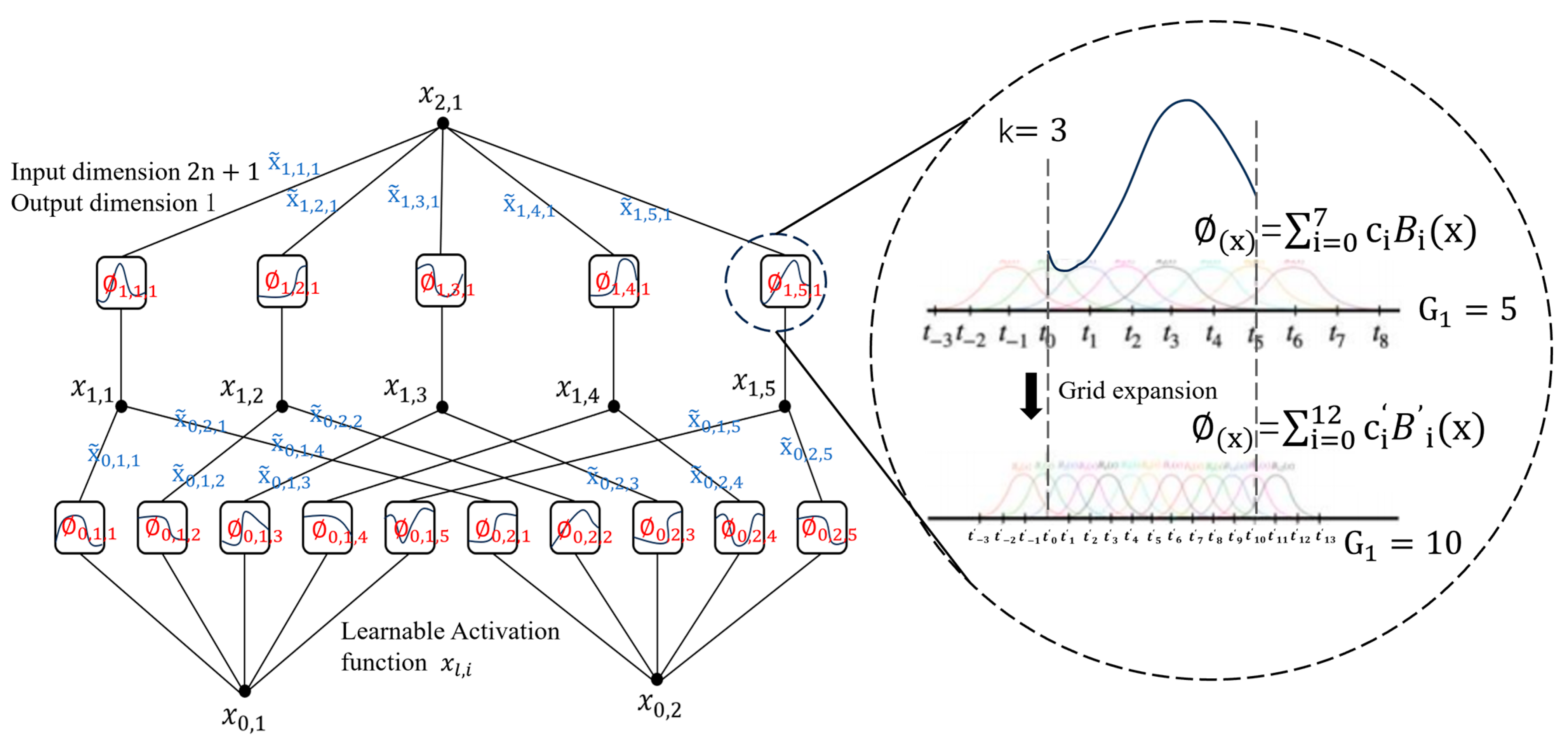
2.2. Principles of the Kolmogorov-Arnold Networks (KAN) Network Algorithm

KAN, short for Kolmogorov-Arnold Networks, is based on the Kolmogorov-Arnold theorem. A distinctive feature of KAN is the placement of learnable activation functions on the network periphery. The fundamental concept is that any continuous multivariate function defined on a bounded domain can be represented as a composite of a finite number of univariate continuous functions combined by addition. More specifically, for a function $f:{\left[\mathrm{0,1}\right]}^n\to R$

$$\mathrm{f}\left(\mathrm{x}\right)=\mathrm{f}\left({\mathrm{x}}_1,\dots ,{\mathrm{x}}_{\mathrm{n}}\right)={\sum }_{\mathrm{q}=1}^{2\mathrm{n}+1}{\mathsf{\Phi }}_{\mathrm{q}}({\sum }_{\mathrm{p}=1}^{\mathrm{n}}{\mathrm{\varnothing }}_{\mathrm{q},\mathrm{p}}({\mathrm{x}}_{\mathrm{p}}))$$

(7)

where each ${\mathrm{\varnothing }}_{q,p}:\left[\mathrm{0,1}\right]\to R$ and ${\mathsf{\Phi }}_q:R\to R$ is a univariate continuous function.

Unlike the fully connected layers in LSTMs—which perform nonlinear spatial transformations at each layer—KAN typically employs B-splines for parameterization. It applies nonlinear transformations to each pair of basis functions individually and then combines them into a multidimensional space. Consequently, a high-dimensional function can be reduced to learning a polynomial number of one-dimensional functions, thereby enhancing both the accuracy and interpretability of KAN when handling complex functions. Graphically, the KAN can be represented as a two-layer neural network without linear combinations, with nonlinear activations applied directly to the input features.

In the “activation layer” of the KAN, multiple B-spline functions with varying numbers of control points are used to approximate functions of arbitrary shapes. Simultaneously, each weight parameter is parameterized as a univariate spline function. As illustrated in Figure 2, the left side shows the activation symbols passing through the KAN network, while the right side displays the activation function parameterized as B-splines, which can toggle between coarse-grained and fine-grained grids [13]. A spline function is a piecewise polynomial that maintains a high degree of smoothness at the junctions (nodes) where polynomial segments meet. This property enables the KAN network to capture local features and trends in the input data. Each decomposed univariate function is responsible for one dimension or feature of the input, and these functions are combined via addition. This approach simplifies the computation of complex functions and enhances the model’s expressive power.

KAN networks optimize their learnable parameters—including the coefficients of the spline functions—using forward and backpropagation algorithms to approximate the target function. During training, the network adjusts its parameters based on changes in the loss function, gradually driving the output closer to its true value.

The “output layer” of the KAN converts the processed results from the hidden layers into the final output. In classification tasks, this layer typically includes activation functions, such as softmax, to produce a probability distribution; in regression tasks, it directly outputs the predicted values. The structure of the KAN network is highly amenable to visualization, facilitating an intuitive understanding and interpretation of the network behavior and results.

In summary, the multi-layer KAN network structure leverages learnable edge activation functions along with function decomposition and recombination to effectively address complex multivariate problems. This makes it particularly well-suited for predicting stress in large-diameter pipelines with various nonlinear characteristics, offering high accuracy, strong interpretability, and excellent flexibility and adaptability.

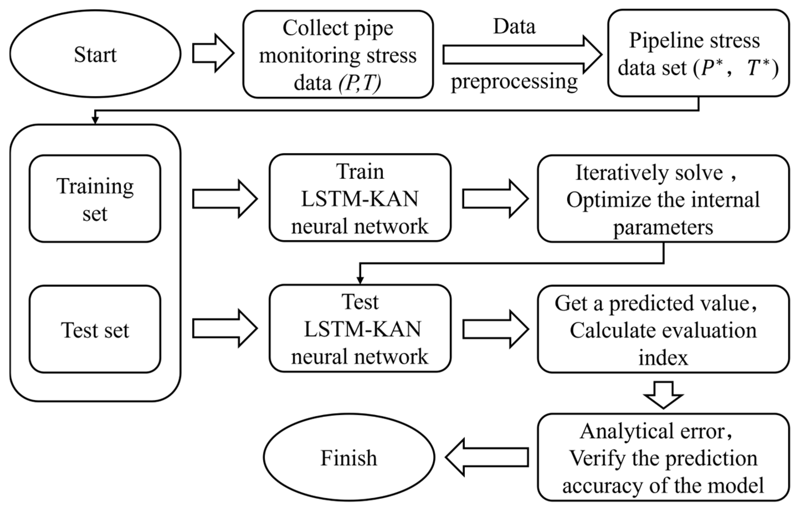
2.3. LSTM-KAN Stress Prediction Model

The LSTM-KAN model combines the LSTM’s ability to process sequential data with the strengths of KAN in modeling complex nonlinear relationships. This integration ensures that the model effectively captures both the temporal dynamics of the data and the nonlinear characteristics of the pipeline stress. Specifically, the traditional fully connected layer in the LSTM is replaced by the KAN. The LSTM layer captures long-term dependencies within the time series, while the KAN layer refines this information using flexible basis function activations and piecewise polynomial weights, allowing it to model the highly nonlinear patterns associated with pipeline stress. Compared to the traditional LSTM model, the LSTM-KAN model increases the number of basis functions in KAN (the number of β-spline basis functions) and the degree of the basis functions. The total number is 4h (k + 1), where h is the hidden layer dimension, and k is the number of KAN basis functions. Additionally, the model parameters include the input size, hidden layer dimension, number of hidden layers, learning rate, and output size.

Additionally, the configuration of the KAN layer involves setting parameters such as the grid size, polynomial order, scaling noise, and activation function scaling. These parameters collectively govern the model’s complexity and adaptability. In this pipeline stress prediction model, in addition to using pipeline stress as an input, additional features, such as frequency, current variation, cumulative variation, and temperature, are incorporated, making each data instance consist of five features. Compared to traditional univariate LSTM models, this multivariate approach enhances prediction accuracy. At the same time, the LSTM-KAN model significantly improves the accuracy and robustness of pipeline stress prediction through adaptive nonlinear modeling, multi-scale feature fusion, and integration of physical constraints. Additionally, its lightweight design helps control computational costs, providing more reliable decision support for pipeline health management.

In the code implementation, the LSTM-KAN model class is defined, and which class named LSTM is created, inheriting from torch.nn.Module, to define the LSTM layer, torch.nn.Module is the base class for all custom neural network layers in PyTorch. For processing the LSTM outputs, the conventional MLP fully connected layer is replaced with a KAN model (also inheriting from torch.nn.Module), with its hidden layer dimension set to 64. In the forward propagation function, the final hidden state of the LSTM serves as the input to the KAN layer, enabling the model to process nonlinear datasets and further enhancing its ability to model nonlinearity in predictions.

Using Hyperopt-based Bayesian optimization in the continuous parameter space, we found the optimal settings to be a time-step length of 10, two hidden layers, a hidden layer dimension of 64, a learning rate of 0.0001, and 200 training epochs. The input feature dimension is set to 5 using argparse.ArgumentParser().add_argument(), ensuring that each data sample, consisting of five features, is used as input, with the output feature dimension set to 1.

The KAN layer is based on piecewise polynomial weights with an optional independent scaling factor. It internally manages the grid generation, weight initialization, and regularization loss computation. The calculation of the piecewise polynomial weights considers factors such as the grid step size, scaling noise, and influence of the basic activation function. This is achieved through methods like curve2coeff, curve2coef is a custom library function whose role is to convert curve parameters into a weight matrix for forward propagation. Furthermore, the KAN layer supports the computation of regularization losses, including L1 and entropy regularization terms, to prevent overfitting and improve the model generalization ability.

The modeling process and structure of the LSTM-KAN model are illustrated in Figure 3, and the pipeline stress prediction process is shown in Figure 4. Predicting pipeline stress typically requires consideration of multiple variables beyond stress measurements, including temperature, pressure, and flow rate. However, LSTM-based pipeline stress prediction models capture only the time-series dynamics at individual sensor locations and thus fail to model the nonlinear interactions among these auxiliary variables, resulting in suboptimal accuracy and limited generalizability.

Large-diameter sewage pipelines often exhibit various nonlinear characteristics during stress monitoring. For example, variations in soil constraint tightness, pipeline−soil separation, and differences in local compaction can cause nonlinear stress concentrations. Extended external conditions and sensor operation may induce nonlinear coupling effects between thermal stress, internal sewage pressure, and flow velocity [21]. Additionally, vibratory string sensors used for monitoring stress may experience nonlinear drift under large deformations or high-frequency vibrations. These nonlinear factors make accurate pipeline stress prediction challenging [22]. By combining LSTM with KAN, the KAN network’s ability to process multivariate data can better capture the complex relationships among variables, allowing the LSTM-KAN model to more effectively model the nonlinear relationships between pipeline stress and various factors, thereby improving prediction accuracy.

The specific implementation steps are as follows: 1. Data collection: Pipeline stress monitoring data are gathered in chronological order, and Kalman filtering is applied to the raw data. 2. Feature processing: The preprocessed dataset is standardized and normalized. 3. Model construction: The LSTM-KAN model is built by adjusting the training parameters, feature weights, and other variables. 4. Training: The dataset is split, and the LSTM-KAN model is trained to predict the pipeline stress, evaluating the model performance using accuracy metrics. 5. Iteration: Steps 3 and 4 are repeated to fine-tune the model parameters, reduce the loss, and improve the accuracy. Training is stopped when the validation loss reduction in five consecutive parameter adjustments is less than 0.5% and the standard deviation of the prediction error is less than 1%. 6. Comparison: The LSTM-KAN model’s prediction results are compared with those of the traditional LSTM model to assess the model’s performance in predicting the actual pipeline stress values.

In order to more accurately and conveniently judge the prediction performance of the model, the following error metrics are used to evaluate model accuracy: Mean Absolute Error (MAE), Root Mean Square Error (RMSE), and the coefficient of determination (R²):

$$\mathrm{M}\mathrm{A}\mathrm{E}={\displaystyle \frac{1}{\mathrm{n}}}{\sum }_{\mathrm{i}=1}^{\mathrm{n}}{|\mathrm{y}}_{\mathrm{i}}-{\widehat{\mathrm{y}}}_{\mathrm{i}}|$$

(8)

$$\mathrm{R}\mathrm{M}\mathrm{S}\mathrm{E}=\sqrt{{\displaystyle \frac{1}{\mathrm{n}}}{\sum }_{\mathrm{i}=1}^{\mathrm{n}}{({\mathrm{y}}_{\mathrm{i}}-{\widehat{\mathrm{y}}}_{\mathrm{i}})}^2}$$

(9)

$${\mathrm{R}}^2=1-{\displaystyle \frac{{\sum }_{\mathrm{i}=1}^{\mathrm{n}}{({\mathrm{y}}_{\mathrm{i}}-{\widehat{\mathrm{y}}}_{\mathrm{i}})}^2}{{\sum }_{\mathrm{i}=1}^{\mathrm{n}}{({\mathrm{y}}_{\mathrm{i}}-\overline{\mathrm{y}})}^2}}$$

(10)

Here, ${\mathrm{y}}_{\mathrm{i}}$ represents the true value, ${\widehat{y}}_i$ represents the predicted value, $\overline{y}$ is the mean of the true values, and n is the sample size. The MAE quantifies the average absolute error between the predictions and true values, with a smaller MAE indicating higher model precision. The RMSE measures the square root of the average squared error, reflecting the magnitude of the prediction error. A lower RMSE indicates better accuracy of the model. The coefficient of determination $R^2$ is a statistical measure that assesses the goodness of fit of the regression model, representing the proportion of variance in the dependent variable explained by the independent variables. A value closer to 1 indicates a better model performance.

3. Research Applications

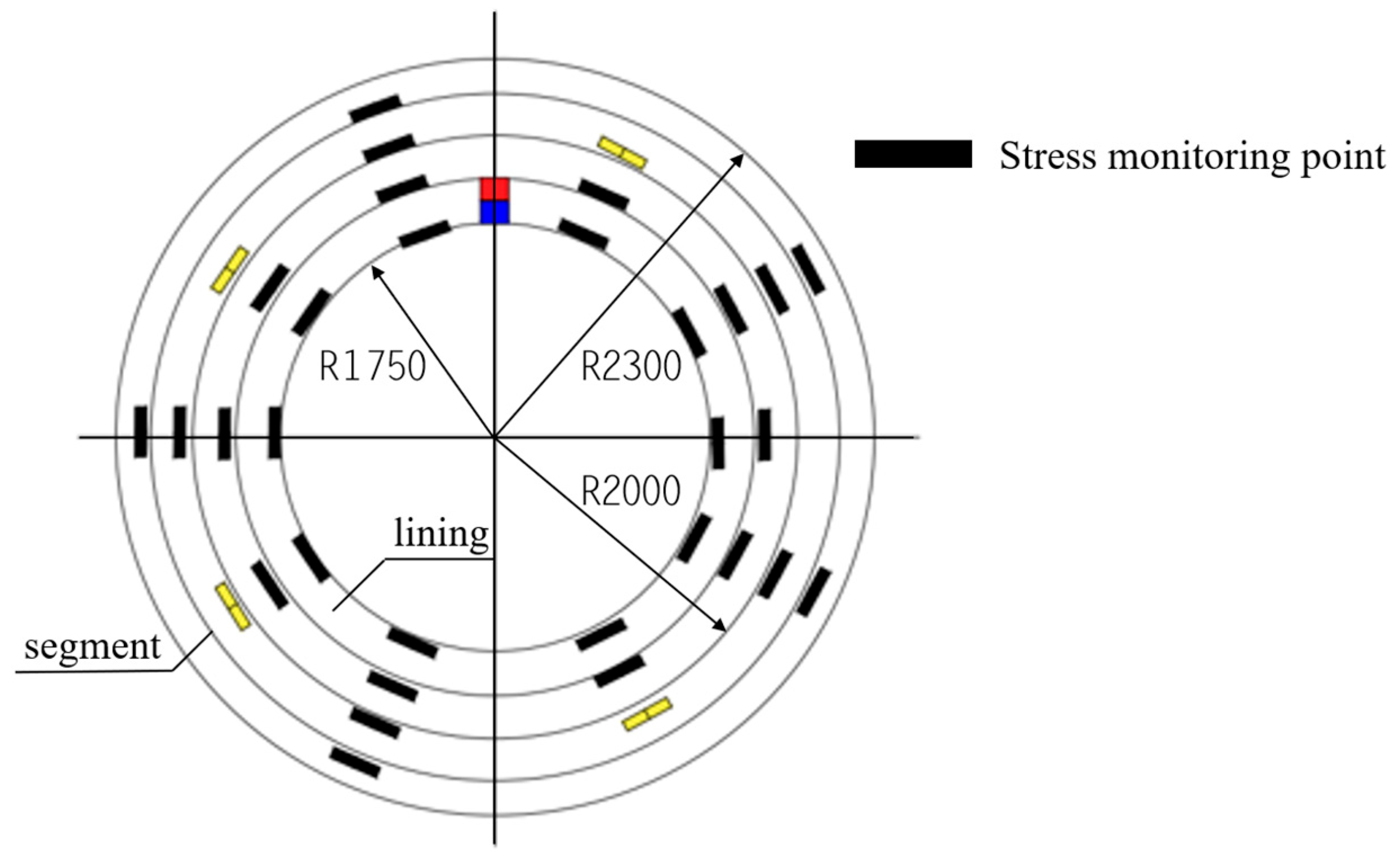
3.1. Project Background

This project involves constructing the Zhuyuan–Bailonggang wastewater interconnection pipeline between the Zhuyuan and Bailonggang wastewater systems. The pipeline is constructed using a combination of pipe-jacking and shield tunneling methods. The selected pipeline diameters are DN3500 for both shield and pipe-jacking sections and 2×DN2400 for additional pipe-jacking sections. Along the route, 31 wells (for pipe-jacking and shield tunneling) are installed, along with six gate wells and 16 ventilation wells.

As shown in Figure 5, the pipeline wall is 550 mm thick, comprising a 300 mm-thick precast segment and a 250 mm-thick lining, both constructed of reinforced concrete. To guard against damage to the sensors embedded in the segments and subsequent sensor failure, auxiliary sensors are also installed within the lining. Internal force monitoring is performed using vibratory string sensors. Each circumferential ring includes 30 monitoring points, which are distributed circumferentially on the inner and outer reinforcements of the top, bottom, and sides of each lining ring. These points are located on the inner and outer reinforcements at the center of each segment, at positions corresponding to the lining monitoring points, and along the segment joints. At each cross-section, the strain gauges from 30 monitoring points are connected to a single data acquisition instrument and conversion module. A single data cable per cross-section extends to a buried junction box that houses a 64-channel data acquisition instrument. The 30 strain gauge signals are converted into 485/232 digital signals and transmitted via a network cable or optoelectronic conversion to an external data acquisition box at the inlet, which is then relayed via 4G/5G wireless transmission to a system data server or cloud server.

For this study, six monitoring points around one circumference of the pipeline were selected for the data analysis and prediction. Data were collected from 11 June–20 September 2024, with each monitoring point recording between 300 and 450 data entries.

3.2. Data Preprocessing and Model Parameter Settings

Training a neural network requires a dataset with sufficiently large and well-labeled features. The raw data comprise five features: pipeline stress, monitoring frequency, current variation, cumulative variation, and temperature. The data are first sorted by monitoring time and then preprocessed using a Kalman filter for noise reduction.

The Kalman filter is a recursive algorithm that updates state estimates based on previous estimates and current measurements, making it highly efficient for processing continuous data streams. It adapts to different system models through the covariance of the measurement and process noise, thereby providing stable estimates in various noisy environments. Under the assumption of Gaussian noise, the Kalman filter produces a minimum mean square error state estimate, making it the optimal estimator for linear Gaussian systems [23,24]. The computations are as follows:

State Update Equation:

$${\mathrm{X}}_{\mathrm{i}+1}=\left(1-{\mathrm{K}}_{\mathrm{i}+1}\right){\mathrm{X}}_{\mathrm{i}}+{\mathrm{K}}_{\mathrm{i}+1}{\mathrm{Z}}_{\mathrm{i}+1}$$

(11)

where

• $X_{i+1}$ is the updated state estimate,
• $X_i$ is the predicted state estimate,
• $Z_{i+1}$ is the measurement at time i+1
• $K_{i+1}$ is the Kalman gain, which weights the predicted estimate and the new measurement.

Kalman Gain Equation:

$$K_{i+1}={\displaystyle \frac{P_i+Q}{P_i+Q+R}}$$

(12)

where

• $P_i$ is the predicted error covariance (a measure of uncertainty in the predicted state),
• $\mathrm{Q}$ is the process noise covariance (representing uncertainty in the system dynamics), and
• $R$ is the measurement noise covariance (representing uncertainty in the measurement process).

To facilitate neural network processing and prevent abnormal gradient fluctuations, the pipeline stress values are normalized using min–max normalization:

$$P^{*}={\displaystyle \frac{(P-P_{min})}{(P_{max}-P_{min})}}$$

(13)

where

• $P^{\mathrm{*}}$ is the normalized pipeline stress, and $\mathrm{P}$ is the actual pipeline stress.

Figure 6 and Figure 7 summarize the stress data from the six monitoring points, with the dataset divided into training and prediction sets at an 8:2 ratio. Figure 6 shows the raw measurements, and Figure 7 shows the data after Kalman filter denoising. The numbers in the upper right corners of Figure 6 and Figure 7 denote the indices of the six different monitoring points. Due to environmental interference and sensor noise, the raw data exhibit pronounced fluctuations and a jagged profile. In contrast, Kalman filtering isolates the true stress signal from noise by removing disturbances while preserving the signal’s physical characteristics, thereby smoothing the curve and improving the overall data reliability and accuracy.

3.3. Model Parameter Settings

In the model, the LSTM layer and the KAN processing layer are implemented as a subclass of torch.nn.Module, with the KAN hidden layer dimension set to 64. The model is configured with a time step of 10, 2 hidden layers, a hidden dimension of 64, a learning rate of 0.0001, and 200 training epochs. The input feature dimension is set to 5, and the output feature dimension is set to 1.

4. Results and Discussion

The experimental results presented in this study provide compelling evidence that the proposed LSTM-KAN model significantly enhances the accuracy and robustness of stress prediction in large-diameter sewage pipelines.

Figure 8 shows the training results of the two model types for stress prediction at the six monitoring points using the training dataset. Figure 8a–f corresponds to the six distinct monitoring points, and to facilitate a clearer comparison of the models’ curves, approximately 20 days of data for each point are displayed. The results clearly indicate that whether stress exhibits continuous fluctuations or abrupt changes, the predicted trends largely mirror the actual measurements. This observation confirms that both the LSTM and LSTM-KAN models effectively capture the temporal dependencies and dynamic characteristics inherent in the deformation processes of sewage pipelines. Notably, the close alignment of the predicted trends with the observed data during training suggests that the models have internalized the complex relationships between the input features and stress variations, which is critical for reliable performance on unseen test datasets [25,26].

Figure 9 presents the post-training predictions of the two model types for the same six monitoring points; likewise, to highlight differences between the models’ forecasts, about 10 days of data per monitoring point are shown. A closer examination of the prediction outcomes, as illustrated in Figure 9, reveals marked differences between the traditional LSTM model and the LSTM-KAN hybrid model. While the LSTM model adeptly captures the overall trend, its predictions often deviate significantly from the actual measurements at individual time points—especially during abrupt stress changes—resulting in notable errors. In contrast, the LSTM-KAN hybrid model consistently produces predictions that not only follow the overall trend but also closely match the observed stress values at each monitoring point. As summarized in

Table 1. The prediction results of the LSTM-KAN model at different monitoring points.

	46–19	46–27	46–34	46–37	54–22	54–32
MAE	0.034	0.033	0.032	0.032	0.033	0.032
RMSE	0.039	0.036	0.036	0.034	0.035	0.034
R2	0.921	0.933	0.935	0.917	0.932	0.931

, the hybrid model achieves a coefficient of determination (R²) exceeding 0.9 across all monitoring points, with both the root mean square error (RMSE) and mean absolute error (MAE) maintained below 0.1. These metrics collectively demonstrate that the LSTM-KAN model delivers stable and high-accuracy predictions with minimal deviation from the observed values.

To evaluate the effectiveness of the proposed LSTM-KAN model, we compared it with the traditional LSTM and CNN models. All three models were trained over multiple rounds using the same dataset to ensure comparable training results. After training, the models predicted the pipeline stress data at six monitoring points, as shown in

Table 2. Evaluation metrics for different models.

	MAE	RMSE	R2
CNN	0.10	0.11	0.51
LSTM	0.09	0.10	0.57
LSTM-KAN	0.033	0.035	0.92

. Compared to the traditional LSTM model, the LSTM-KAN reduced the MAE and RMSE by 63.33% and 65%, respectively, while increasing R² by 38.04%. Compared to the CNN model, the MAE and RMSE were reduced by 67% and 68.2%, respectively, and the R² increased by 44.57%. The results indicate that the LSTM model slightly outperforms the CNN model across the three metrics, while the LSTM-KAN model significantly outperforms LSTM on all metrics. This improvement is primarily due to CNN’s stronger ability to extract spatial features but weaker capacity to model long-term dependencies in time-series data [27]. In contrast, during the training process, the KAN layer in LSTM-KAN continuously optimizes the parameters based on the changes in the loss function, making the predictions more accurate and closer to the true values.

Further evidence of the model’s efficacy is provided by the X-Y error scatter plot in Figure 10, where the actual stress values (horizontal axis) are compared with the predicted values (vertical axis) against the reference lines at Y = X and Y = X ± 0.2. As shown in the plot, most of the predicted values of the LSTM-KAN model at the six monitoring points are concentrated near Y = X and fall within the Y = X ± 0.2 range. In contrast, only a few points of the LSTM and CNN models are near Y = X, and many predicted values fall outside the Y = X ± 0.2 range, with CNN showing a particularly high occurrence of values beyond this range. This indicates that, compared to LSTM and CNN, the LSTM-KAN model can more accurately predict pipeline stress, with its prediction errors being evenly distributed and within a reasonable range without significant systematic bias. In addition, it underscores the model’s strong generalization capabilities and minimizes the risk of localized prediction failures.

Moreover, the analysis of the training dynamics, as depicted in Figure 11, shows the number of epochs each of the two models requires to approach its minimum loss; the fewer the epochs, the higher the model’s accuracy and efficiency. The results show that as both models approach their minimum loss values, the LSTM-KAN model converges significantly faster, requiring fewer epochs than the traditional LSTM model. This rapid convergence indicates improved training efficiency, reduced training time and computational costs, reduced overfitting, and more efficient utilization of computational resources, which are crucial for large-scale, real-time monitoring systems.

Figure 12 provides a detailed breakdown of the evaluation metrics for each of the six monitoring points. The comprehensive performance data consistently demonstrate that the LSTM-KAN model outperforms the conventional LSTM model and CNN model across all key indicators. By decomposing and recombining individual univariate functions and continuously optimizing their learnable activation functions, the KAN component captures both local features and global trends more effectively than traditional fully connected layers. This capability is vital for managing the inherent nonlinearity and variability in pipeline stress data, thereby enabling the model to detect subtle changes that might otherwise be overlooked.

In addition to employing more suitable predictive metrics, the LSTM-KAN model has several additional advantages. By incorporating multiple feature inputs, it captures the interrelationships among diverse stress-inducing factors, thereby improving adaptability to new data environments and preserving robustness across different operating conditions. Furthermore, continuous parameter optimization within the KAN layer enhances the prediction process, yielding more reliable and accurate stress forecasts.

The integration of the KAN layer also provides built-in feature scaling and transformation capabilities, which are particularly beneficial when the input data exhibit high variability or nonlinearity. The KAN layer’s dynamic upsampling mechanism further amplifies critical feature variations, increasing the model’s sensitivity to subtle yet significant changes in stress levels. Together, these attributes underscore the technical strengths of the LSTM-KAN model and its potential for high-precision and stable stress prediction in large-diameter sewage pipelines.

5. Conclusions

The proposed LSTM time-series model integrates the KAN network architecture with an upsampler to address the practical challenge of pipeline stress prediction, demonstrating high accuracy and excellent generalizability. Although both the standard LSTM and LSTM-KAN hybrid models can be employed for this task, our findings indicate that the LSTM-KAN model offers superior fitting capability, higher prediction accuracy, and lower loss, particularly when processing long-term data. This improvement is largely attributable to the KAN layer’s capacity to learn dynamic activation functions that adapt to complex input variations, thereby capturing subtle stress fluctuations that are often missed by conventional methods.

• Compared with traditional fully connected layers, the KAN layer achieves higher prediction accuracy using fewer parameters and less training time, underscoring its potential not only for pipeline stress prediction but also for a broad range of forecasting applications. Moreover, the modular nature of the LSTM-KAN architecture enables it to be scaled for deeper and larger-scale tasks. By optimizing the structure and parameters of the KAN layer, both the prediction quality and computational efficiency can be further enhanced, which is an essential feature for real-time monitoring in large infrastructures.
• By combining the long-term memory capabilities of LSTM with the nonlinear representation power of KAN, the hybrid model effectively addresses the challenges posed by time-series data and the nonlinear complexities encountered in practical scenarios. Adjustments in the grid size and selection of appropriate activation functions allow for fine-tuning of the model’s flexibility and customizability, ensuring reliable performance across diverse data distributions and operational conditions.
• Future research should systematically investigate the model performance under varied parameter settings, including the impact of different depths and complexities of the KAN layer on both prediction accuracy and computational efficiency. Additionally, integrating supplementary data sources—such as environmental factors or historical maintenance records—may further enhance the model’s predictive power; investigating the applicability of this model for predicting stresses in sewage pipes with diverse functions and materials—such as prefabricated plastics (e.g., PVC or HDPE)—constitutes a promising direction for future research.

In summary, the LSTM-KAN hybrid model represents a significant advancement in pipeline stress prediction. Its enhanced performance, reduced computational cost, and scalability make it a promising tool for proactive maintenance and risk management of critical infrastructure. Continued refinement and exploration of its integration with other advanced deep learning techniques could pave the way for more reliable and efficient predictive maintenance systems, ultimately contributing to improved structural health monitoring in various applications.

References

1. Das, S.; Saha, P. Structural health monitoring techniques implemented on IASC–ASCE benchmark problem: A review. J. Civ. Struct. Health Monit. 2018, 8, 689–718. [Google Scholar] [CrossRef]
2. Rauch, W.; Bertrand-Krajewski, J.-L.; Krebs, P.; Mark, O.; Schilling, W.; Schütze, M.; Vanrolleghem, P. Deterministic modelling of integrated urban drainage systems. Water Sci. Technol. 2002, 45, 81–94. [Google Scholar] [CrossRef] [PubMed]
3. Xu, C. Research on Non-invasive Detection Method of Pipeline Pressure Based on Fiber Bragg Grating. Master’s Thesis, China University of Petroleum, Beijing, China, 2018. [Google Scholar]
4. Hu, B.; Zhou, M.; Li, Y. Real-time Stress Acquisition Method of In-service Pipe Based on Vibration Measurement. Agric. Equip. Veh. Eng. 2017, 55, 47–48+55. [Google Scholar]
5. Zhang, H. Study on Stress Analysis and Monitoring Technology of Pipeline Landslide. Master’s Thesis, China University of Petroleum, Beijing, China, 2019. [Google Scholar]
6. He, Y. Research on Long-Distance Pipeline Distributed Stress Monitoring and Health Diagnosis Method. Master’s Thesis, Wuhan Institute of Technology, Wuhan, China, 2015. [Google Scholar]
7. El-Abbasy, M.S.; Senouci, A.; Zayed, T.; Mirahadi, F.; Parvizsedghy, L. Artificial neural network models for predicting condition of offshore oil and gas pipelines. Autom. Constr. 2014, 45, 50–65. [Google Scholar] [CrossRef]
8. Liu, Y.; Yu, Z.; Tong, L. Early Warning Model of Pipeline Stress State Based on Axial Stress Monitoring Data. China Pet. Mach. 2018, 46, 105–109. [Google Scholar]
9. Goodfellow, I.; Bengio, Y.; Courville, A.; Bengio, Y. Deep Learning; MIT Press: Cambridge, UK, 2016. [Google Scholar]
10. Hochreiter, S.; Schmidhuber, J. Long short-term memory. Neural Comput. 1997, 9, 1735–1780. [Google Scholar] [CrossRef] [PubMed]
11. Graves, A. Supervised Sequence Labelling with Recurrent Neural Networks; Springer: Berlin/Heidelberg, Germany, 2012. [Google Scholar] [CrossRef]
12. Leng, J.; Qian, W.; Zhou, L. Experimental Study on Safety Warning of Oil and Gas Pipeline Based on Stress Monitoring. China Pet. Mach. 2021, 49, 139–144. [Google Scholar]
13. Liu, X. Research on pipeline stress prediction and early warning technology based on ARIMA-LSTM. Pet. Eng. Constr. 2022, 48, 38–43. [Google Scholar]
14. Liu, Z.; Wang, Y.; Vaidya, S.; Ruehle, F.; Halverson, J.; Soljačić, M.; Hou, T.Y.; Tegmark, M. Kan: Kolmogorov-Arnold networks. arXiv 2024, arXiv:2404.19756. [Google Scholar]
15. Chen, S.; Ge, L. Exploring the attention mechanism in LSTM-based Hong Kong stock price movement prediction. Quant. Financ. 2019, 19, 1507–1515. [Google Scholar] [CrossRef]
16. Liu, W.; Lu, H.; Fu, H.; Cao, Z. Learning to Upsample by Learning to Sample. In Proceedings of the IEEE/CVF International Conference on Computer Vision, Paris, France, 1–6 October 2023. [Google Scholar]
17. Zhou, L.; Leng, J.; Wei, L. Early Warning Technology of Oil and Gas Pipeline Based on Monitoring Data. Press. Vessel Technol. 2019, 36, 55–60. [Google Scholar]
18. Bian, X.; Cheng, Y.; Bai, X. HW-CSC Stress-strain Model and Its Application in Strength Prediction. Chin. J. Undergr. Space Eng. 2021, 17, 1782–1788. [Google Scholar]
19. Yang, B.; Yin, K.; Lacasse, S.; Liu, Z. Time series analysis and long short-term memory neural network to predict landslide displacement. Landslides 2019, 16, 677–694. [Google Scholar] [CrossRef]
20. Huang, H.; Guo, P.; Yan, J.; Zhang, B.; Mao, Z. Impact of uncertainty in the physics-informed neural network on pressure prediction for water hammer in pressurized pipelines. J. Phys. Conf. Ser. 2024, 2707, 012095. [Google Scholar] [CrossRef]
21. Soomro, A.A.; Mokhtar, A.A.; Hussin, H.B.; Lashari, N.; Oladosu, T.L.; Jameel, S.M.; Inayat, M. Analysis of machine learning models and data sources to forecast burst pressure of petroleum corroded pipelines: A comprehensive review. Eng. Fail. Anal. 2024, 155, 107747. [Google Scholar] [CrossRef]
22. Seenuan, P.; Noraphaiphipaksa, N.; Kanchanomai, C. Stress Intensity Factors for Pressurized Pipes with an Internal Crack: The Prediction Model Based on an Artificial Neural Network. Appl. Sci. 2023, 13, 11446. [Google Scholar] [CrossRef]
23. Guo, W.; Li, Z.; Gao, C.; Yang, Y. Stock price forecasting based on improved time convolution network. Comput. Intell. 2022, 38, 1474–1491. [Google Scholar] [CrossRef]
24. Zhang, Z.; Wang, Z. Design of financial big data audit model based on artificial neural network. Int. J. Syst. Assur. Eng. Manag. 2021, 1–10. [Google Scholar] [CrossRef]
25. Zhu, X.; Xiong, Y.; Wu, M.; Nie, G.; Zhang, B.; Yang, Z. Weather2k: A multivariate spatio-temporal benchmark dataset for meteorological forecasting based on real-time observation data from ground weather stations. arXiv 2023, arXiv:2302.10493. [Google Scholar]
26. Li, X.; Jing, H.; Liu, X.; Chen, G.; Han, L. The prediction analysis of failure pressure of pipelines with axial double corrosion defects in cold regions based on the BP neural network. Int. J. Press. Vessel Pip. 2023, 202, 104907. [Google Scholar] [CrossRef]
27. Mehtab, S.; Sen, J. Analysis and forecasting of financial time seriesusing cnn and lstm-based deep learning models. In Advances in Distributed Computing and Machine Learning: Proceedings of ICADCML 2021; Springer: Berlin/Heidelberg, Germany, 2022; pp. 405–423. [Google Scholar]
Figure 1. LSTM neuron structure.
Information 16 00347 g001
Figure 2. The framework of KAN.
Information 16 00347 g002
Figure 3. Model Structure of LSTM-KAN.
Information 16 00347 g003
Figure 4. Prediction process of LSTM-KAN.
Information 16 00347 g004
Figure 5. Diagram of Stress Monitoring Points.
Information 16 00347 g005
Figure 6. Raw Data.
Information 16 00347 g006
Figure 7. Preprocessed Data.
Information 16 00347 g007
Figure 8. Training Data. (a) 46–19; (b) 46–27; (c) 46–34; (d) 46–37; (e) 54–22; (f) 54–32.
Information 16 00347 g008
Figure 9. Predicted Data. (a) 46–19; (b) 46–27; (c) 46–34; (d) 46–37; (e) 54–22; (f) 54–32.
Information 16 00347 g009
Figure 10. The error distribution of LSTM-KAN model. (a) 46–19; (b) 46–27; (c) 46–34; (d) 46–37; (e) 54–22; (f) 54–32.
Information 16 00347 g010
Figure 11. Contrast of different models.
Information 16 00347 g011
Figure 12. Comparison of evaluation indicators for different models. (a) MAE; (b) RMSE; (c) R2.
Information 16 00347 g012