
Detecting Driver Drowsiness Using Hybrid Facial Features and Ensemble Learning


Abstract
1. Introduction
- (1)
- To tackle the issue of inaccurate feature extraction due to inter-individual differences among drivers, we developed an adaptive threshold correction method that ensures precise feature extraction across various drivers.
- (2)
- To address the limitations of existing methods that consider a limited set of facial features and struggle to represent the diverse manifestations of drowsiness among different drivers, we designed 20 features spanning four facial regions—the eyes, mouth, head pose, and gaze direction—and implemented a personalized standardization strategy during preprocessing, achieving the comprehensive coverage of the facial region’s features.
- (3)
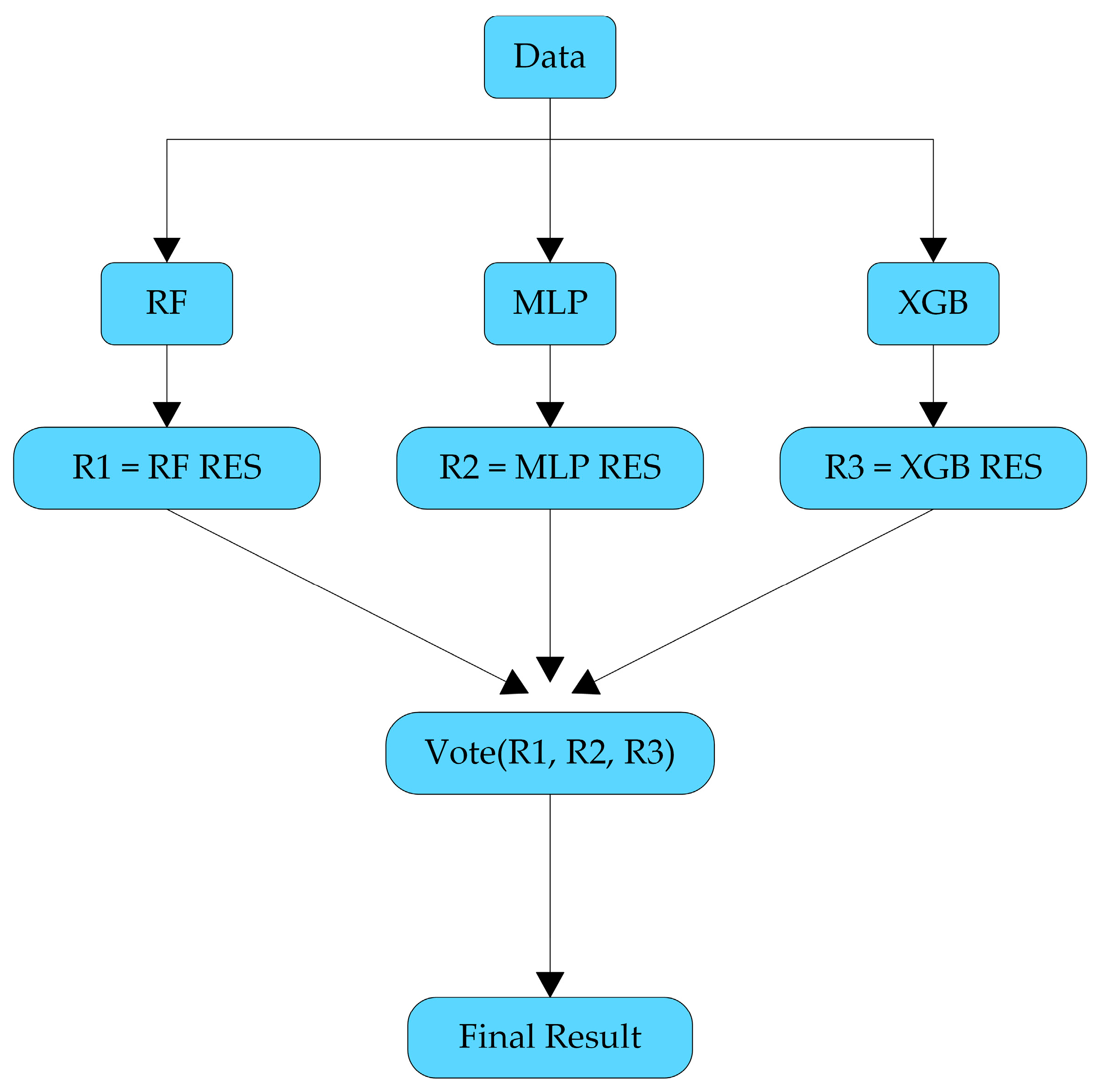
- To overcome the limitations of relying on a single model, we integrated multiple models, combining the strengths of various machine learning techniques to construct a robust and high-precision driver drowsiness detection system.
- (4)
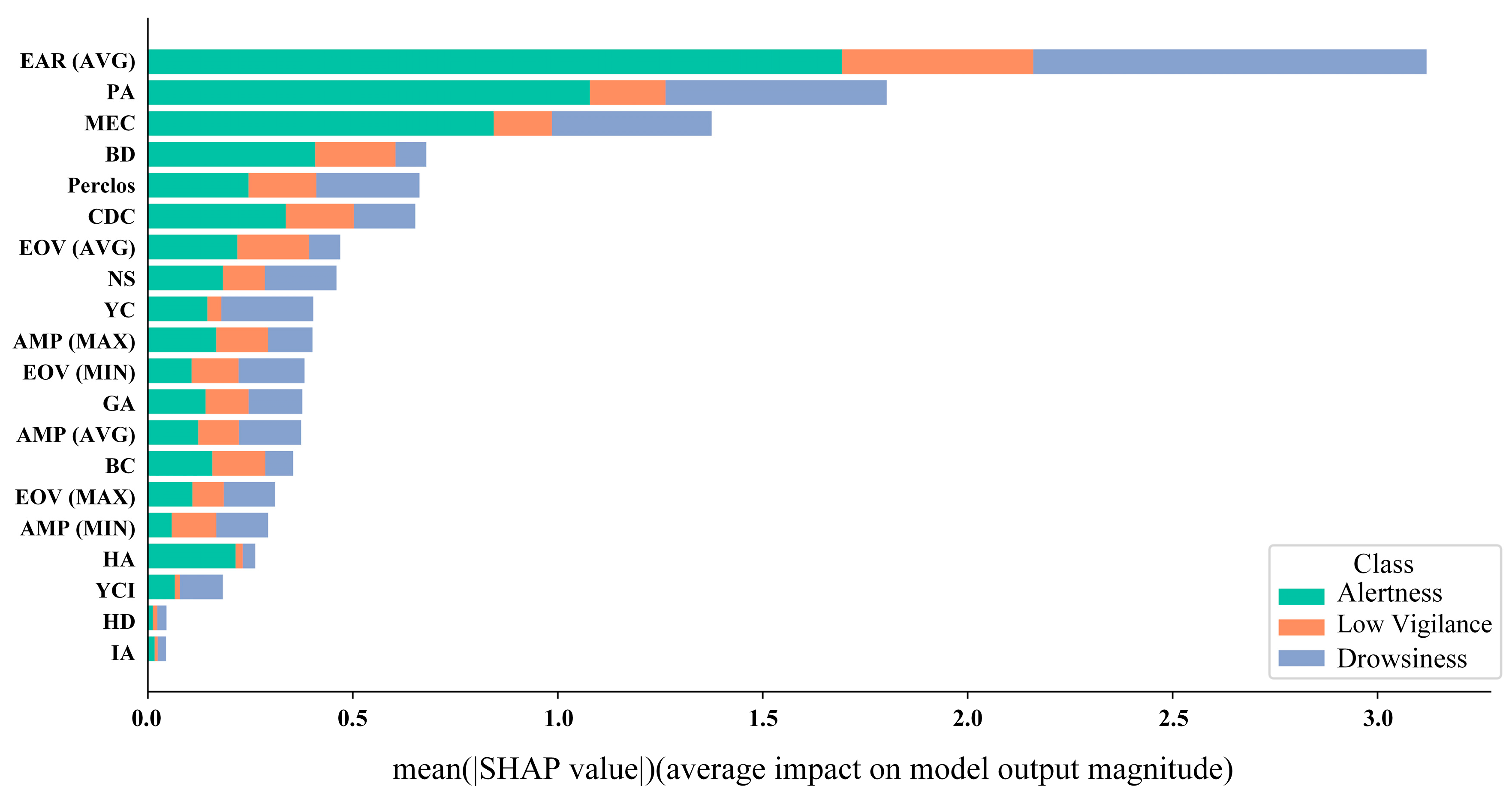
- We employed the Shapley Additive Explanations (SHAP) method to analyze the model’s decision-making process, uncovering the importance of different features in the model’s predictions and providing valuable insights for future research in this field.
2. Materials and Methods
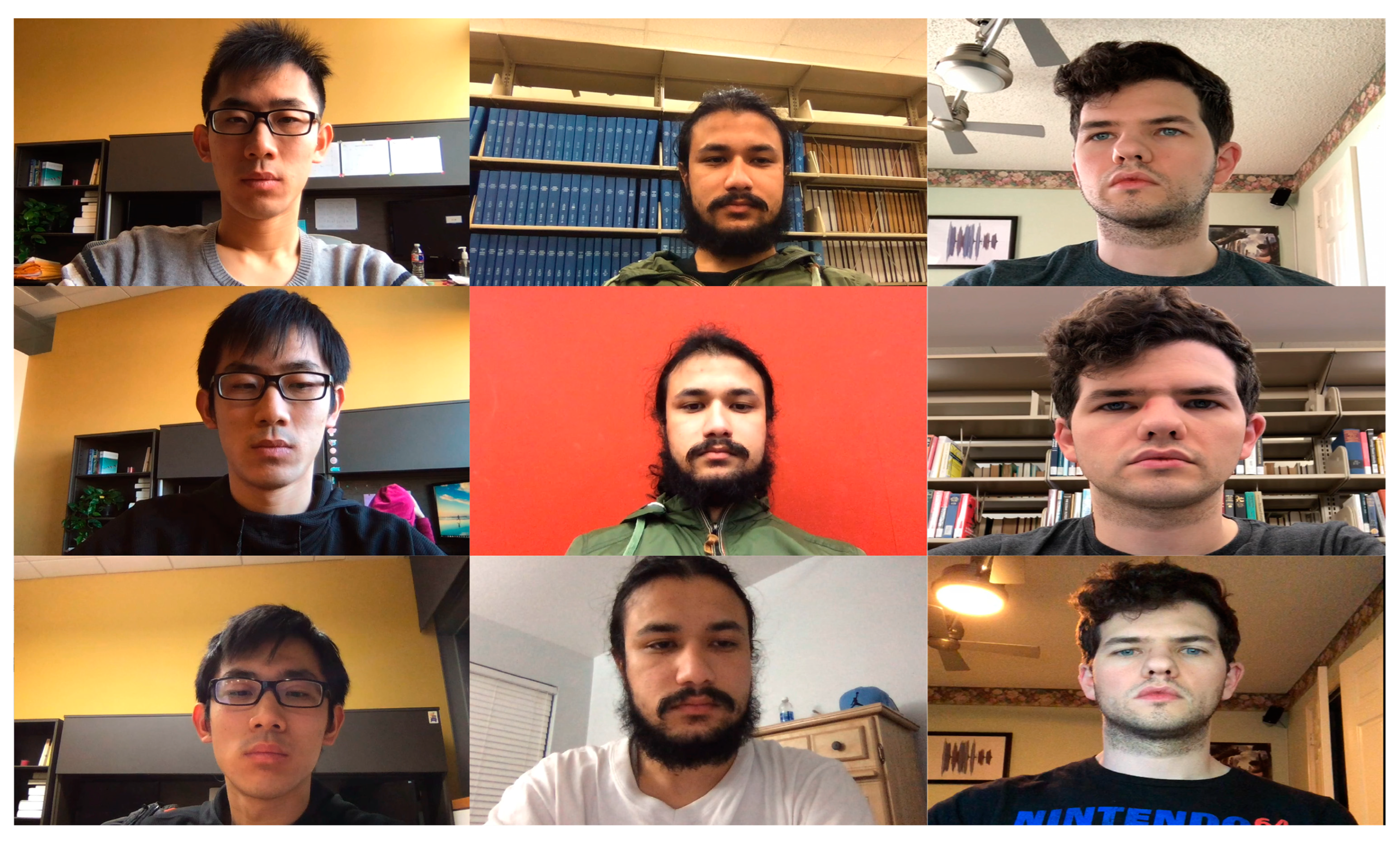
2.1. Dataset
2.2. Feature Extraction
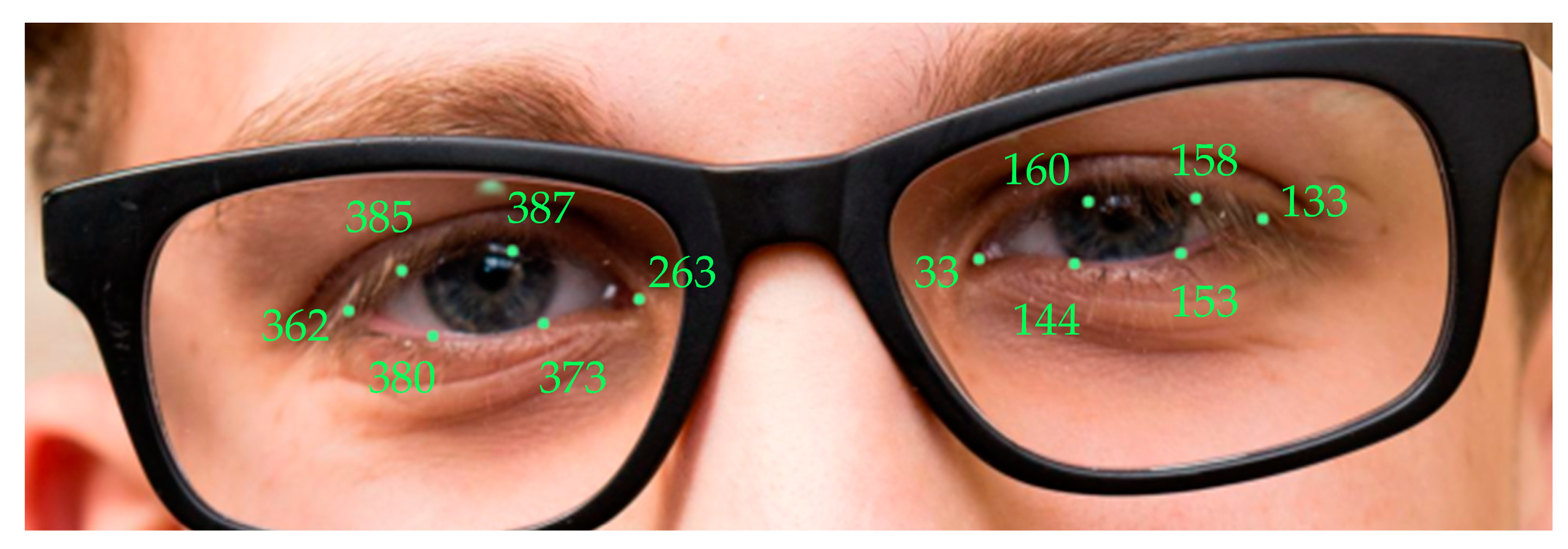
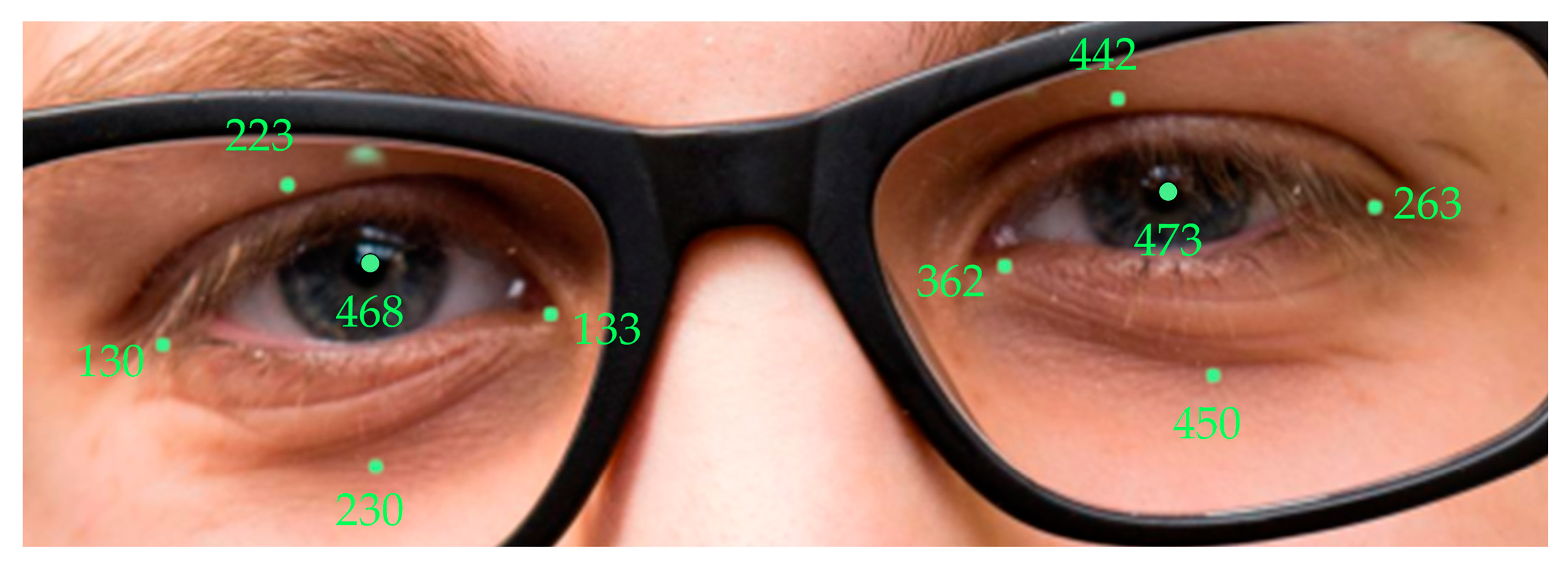
2.2.1. Eye Region Features
2.2.2. Mouth Contour Features
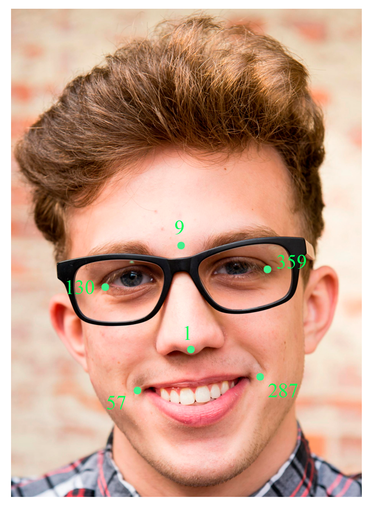
2.2.3. Head Pose Features
2.2.4. Gaze Direction Features
2.3. Adaptive Threshold Correction Method
| Algorithm 1: Adaptive Blink Threshold |
| Input: Eye aspect ratio at time , time window , initial threshold , minimum blink frames . Output:. . |
|
2.4. Data Preprocessing
2.5. Classifiers
2.6. Shapley Additive Explanations (SHAP)
3. Results and Discussion
3.1. Performance Comparison of Different Models
3.2. Performance Comparison of Different Feature Combinations
3.3. Comparison with Similar Techniques
3.4. SHAP Analysis
4. Conclusions
Author Contributions
Funding
Institutional Review Board Statement
Informed Consent Statement
Data Availability Statement
Acknowledgments
Conflicts of Interest
References
- Perkins, E.; Sitaula, C.; Burke, M.; Marzbanrad, F. Challenges of driver drowsiness prediction: The remaining steps to implementation. IEEE Trans. Intell. Veh. 2023, 8, 1319–1338. [Google Scholar]
- Australian Transport Council. National Road Safety Strategy 2011–2020. 2011. Available online: https://www.roadsafety.gov.au/nrss/2011-20 (accessed on 12 February 2025).
- Sikander, G.; Anwar, S. Driver Fatigue Detection Systems: A Review. IEEE Trans. Intell. Transp. Syst. 2019, 20, 2339–2352. [Google Scholar]
- Wang, Q.; Yang, J.; Ren, M.; Zheng, Y. Driver fatigue detection: A survey. In Proceedings of the 2006 6th World Congress on Intelligent Control and Automation, Dalian, China, 21–23 June 2006. [Google Scholar]
- Bekhouche, S.E.; Ruichek, Y.; Dornaika, F. Driver drowsiness detection in video sequences using hybrid selection of deep features. Knowl.-Based Syst. 2022, 252, 109436. [Google Scholar]
- Chai, M. Drowsiness monitoring based on steering wheel status. Transp. Res. Part D Transp. Environ. 2019, 66, 95–103. [Google Scholar] [CrossRef]
- Li, R.; Chen, Y.V.; Zhang, L. A method for fatigue detection based on driver’s steering wheel grip. Int. J. Ind. Ergon. 2021, 82, 103083. [Google Scholar]
- Hasanuddin, M.O.; Novianingrum, H.; Syamsuddin, E.Y. Design and implementation of drowsiness detection system based on standard deviation of lateral position. In Proceedings of the 2022 12th International Conference on System Engineering and Technology (ICSET), Bandung, Indonesia, 3–4 October 2022. [Google Scholar]
- Hu, J.; Xu, L.; He, X.; Meng, W. Abnormal driving detection based on normalized driving behavior. IEEE Trans. Veh. Technol. 2017, 66, 6645–6652. [Google Scholar]
- Latreche, I.; Slatnia, S.; Kazar, O.; Harous, S. An optimized deep hybrid learning for multi-channel EEG-based driver drowsiness detection. Biomed. Signal Process. Control 2025, 99, 106881. [Google Scholar]
- Lin, X.; Huang, Z.; Ma, W.; Tang, W. EEG-based driver drowsiness detection based on simulated driving environment. Neurocomputing 2025, 616, 128961. [Google Scholar]
- Lins, I.D.; Araújo, L.M.M.; Maior, C.B.S.; da Silva Ramos, P.M.; das Chagas Moura, M.J.; Ferreira-Martins, A.J.; Chaves, R.; Canabarro, A. Quantum machine learning for drowsiness detection with EEG signals. Process Saf. Environ. Prot. 2024, 186, 1197–1213. [Google Scholar] [CrossRef]
- Freitas, A.; Almeida, R.; Gonçalves, H.; Conceição, G.; Freitas, A. Monitoring fatigue and drowsiness in motor vehicle occupants using electrocardiogram and heart rate—A systematic review. Transp. Res. Part F Traffic Psychol. Behav. 2024, 103, 586–607. [Google Scholar]
- Fouad, I.A. A robust and efficient EEG-based drowsiness detection system using different machine learning algorithms. Ain Shams Eng. J. 2023, 14, 101895. [Google Scholar]
- Oliveira, L.; Cardoso, J.S.; Lourenço, A.; Ahlström, C. Driver drowsiness detection: A comparison between intrusive and non-intrusive signal acquisition methods. In Proceedings of the 2018 7th European Workshop on Visual Information Processing (EUVIP), Tampere, Finland, 26–28 November 2018. [Google Scholar]
- Zhang, Z.; Ning, H.; Zhou, F. A systematic survey of driving fatigue monitoring. IEEE Trans. Intell. Transp. Syst. 2022, 23, 19999–20020. [Google Scholar]
- Cori, J.M.; Turner, S.; Westlake, J.; Naqvi, A.; Ftouni, S.; Wilkinson, V.; Vakulin, A.; O’Donoghue, F.J.; Howard, M.E. Eye blink parameters to indicate drowsiness during naturalistic driving in participants with obstructive sleep apnea: A pilot study. Sleep Health 2021, 7, 644–651. [Google Scholar] [PubMed]
- Hollander, J.; Huette, S. Extracting blinks from continuous eye-tracking data in a mind wandering paradigm. Conscious. Cogn. 2022, 100, 103303. [Google Scholar]
- Patel, P.P.; Pavesha, C.L.; Sabat, S.S.; More, S.S. Deep Learning based Driver Drowsiness Detection. In Proceedings of the 2022 International Conference on Applied Artificial Intelligence and Computing (ICAAIC), Salem, India, 9–11 May 2022; pp. 380–386. [Google Scholar]
- Cori, J.M.; Wilkinson, V.E.; Jackson, M.; Westlake, J.; Stevens, B.; Barnes, M.; Swann, P.; Howard, M.E. The Impact of Alcohol Consumption on Commercial Eye Blink Drowsiness Detection Technology. Hum. Psychopharmacol. 2023, 38, e2870. [Google Scholar]
- Schmidt, J.; Laarousi, R.; Stolzmann, W.; Karrer-Gauß, K. Eye blink detection for different driver states in conditionally automated driving and manual driving using EOG and a driver camera. Behav. Res. 2018, 50, 1088–1101. [Google Scholar]
- Ramzan, M.; Khan, H.U.; Awan, S.M.; Ismail, A.; Ilyas, M.; Mahmood, A. A survey on state-of-the-art drowsiness detection techniques. IEEE Access 2019, 7, 61904–61919. [Google Scholar]
- Seeck, M.; Koessler, L.; Bast, T.; Leijten, F.; Michel, C.; Baumgartner, C.; He, B.; Beniczky, S. The Standardized EEG Electrode Array of the IFCN. Clin. Neurophysiol. 2017, 128, 2070–2077. [Google Scholar]
- Jiao, Y.; Deng, Y.; Luo, Y.; Lu, B.L. Driver Sleepiness Detection from EEG and EOG Signals Using GAN and LSTM Networks. Neurocomputing 2020, 408, 100–111. [Google Scholar]
- Yang, G.; Lin, Y.; Bhattacharya, P. A Driver Fatigue Recognition Model Based on Information Fusion and Dynamic Bayesian Network. Inf. Sci. 2010, 180, 1942–1954. [Google Scholar]
- Leicht, L.; Ruder, H.; Müller, C.; Suter, R.; Iff, I.; Moser, R.; Stettler, A. Capacitive ECG Monitoring in Cardiac Patients During Simulated Driving. IEEE Trans. Biomed. Eng. 2018, 66, 749–758. [Google Scholar] [CrossRef] [PubMed]
- Walter, M.; Huebner, W.; Kautz, S.; Behrens, M.; Henn, J.; Heuser, L.; Pfeiffer, U.; Hentschel, B.; Reiss, M. The Smart Car Seat: Personalized Monitoring of Vital Signs in Automotive Applications. Pers. Ubiquitous Comput. 2011, 15, 707–715. [Google Scholar] [CrossRef]
- Sun, Y.; Yu, X. An Innovative Nonintrusive Driver Assistance System for Vital Signal Monitoring. IEEE J. Biomed. Health Inform. 2014, 18, 1932–1939. [Google Scholar] [CrossRef] [PubMed]
- Arefnezhad, S.; Samiee, S.; Eichberger, A.; Nahvi, A. Driver Drowsiness Detection Based on Steering Wheel Data Applying Adaptive Neuro-Fuzzy Feature Selection. Sensors 2019, 19, 943. [Google Scholar] [CrossRef] [PubMed]
- Sun, Z.; Zhang, H.; Zhang, Y.; Zhang, W. Facial feature fusion convolutional neural network for driver fatigue detection. Eng. Appl. Artif. Intell. 2023, 126, 106981. [Google Scholar] [CrossRef]
- Rajamohana, S.P.; Radhika, E.G.; Priya, S.; Sangeetha, S. Driver drowsiness detection system using hybrid approach of convolutional neural network and bidirectional long short term memory (CNN_BILSTM). Mater. Today Proc. 2021, 45 Pt 2, 2897–2901. [Google Scholar] [CrossRef]
- El-Nabi, S.A.; El-Shafai, W.; El-Rabaie, E.S.; Ramadan, K.F.; El-Samie, F.E.A.; Mohsen, S. Machine learning and deep learning techniques for driver fatigue and drowsiness detection: A review. Multimed. Tools Appl. 2024, 83, 9441–9477. [Google Scholar] [CrossRef]
- Sahayadhas, A.; Sundaraj, K.; Murugappan, M. Detecting driver drowsiness based on sensors: A review. Sensors 2012, 12, 16937–16953. [Google Scholar] [CrossRef]
- Guo, W.; Zhang, B.; Xia, L.; Shi, S.; Zhang, X.; She, J. Driver drowsiness detection model identification with Bayesian network structure learning method. In Proceedings of the 2016 Chinese Control and Decision Conference (CCDC), Yinchuan, China, 28–30 May 2016; pp. 131–136. [Google Scholar]
- Wang, X.; Xu, C. Driver Drowsiness Detection Based on Non-Intrusive Metrics Considering Individual Specifics. Accid. Anal. Prev. 2016, 95, 350–357. [Google Scholar] [CrossRef]
- Hailin, W.; Hanhui, L.; Zhumei, S. Fatigue driving detection system design based on driving behavior. In Proceedings of the 2010 International Conference on Optoelectronics and Image Processing, Haikou, China, 11–12 November 2010; pp. 549–552. [Google Scholar]
- Takei, Y.; Furukawa, Y. Estimate of driver’s fatigue through steering motion. In Proceedings of the 2005 IEEE International Conference on Systems, Man and Cybernetics, Waikoloa, HI, USA, 12 October 2005; Volume 2, pp. 1765–1770. [Google Scholar]
- Dehzangi, O.; Masilamani, S. Unobtrusive driver drowsiness prediction using driving behavior from vehicular sensors. In Proceedings of the 2018 24th International Conference on Pattern Recognition (ICPR), Beijing, China, 20–24 August 2018; pp. 3598–3603. [Google Scholar]
- McDonald, A.D.; Lee, J.D.; Schwarz, C.; Brown, T.L. A contextual and temporal algorithm for driver drowsiness detection. Accid. Anal. Prev. 2018, 113, 25–37. [Google Scholar] [CrossRef]
- Zhang, X.; Wang, X.; Yang, X.; Xu, C.; Zhu, X.; Wei, J. Driver drowsiness detection using mixed-effect ordered logit model considering time cumulative effect. Anal. Methods Accid. Res. 2020, 26, 100114. [Google Scholar]
- Lu, K.; Sjörs Dahlman, A.; Karlsson, J.; Candefjord, S. Detecting driver fatigue using heart rate variability: A systematic review. Accid. Anal. Prev. 2022, 178, 106830. [Google Scholar] [CrossRef]
- Sun, Y.; Wang, R.; Zhang, H.; Ding, N.; Ferreira, S.; Shi, X. Driving fingerprinting enhances drowsy driving detection: Tailoring to individual driver characteristics. Accid. Anal. Prev. 2024, 208, 107812. [Google Scholar] [PubMed]
- Owen, V.; Surantha, N. Computer vision-based drowsiness detection using handcrafted feature extraction for edge computing devices. Appl. Sci. 2025, 15, 638. [Google Scholar] [CrossRef]
- Makhmudov, F.; Turimov, D.; Xamidov, M.; Nazarov, F.; Cho, Y.-I. Real-time fatigue detection algorithms using machine learning for yawning and eye state. Sensors 2024, 24, 7810. [Google Scholar] [CrossRef]
- Liu, W.; Qian, J.; Yao, Z.; Jiao, X.; Pan, J. Convolutional two-stream network using multi-facial feature fusion for driver fatigue detection. Future Internet 2019, 11, 115. [Google Scholar] [CrossRef]
- Jung, H.-S.; Shin, A.; Chung, W.-Y. Driver fatigue and drowsiness monitoring system with embedded electrocardiogram sensor on steering wheel. IET Intell. Transp. Syst. 2014, 8, 43–50. [Google Scholar] [CrossRef]
- Sahayadhas, A.; Sundaraj, K.; Murugappan, M.; Palaniappan, R. A physiological measures-based method for detecting inattention in drivers using machine learning approach. Biocybern. Biomed. Eng. 2015, 35, 198–205. [Google Scholar]
- Lohani, M.; Payne, B.R.; Strayer, D.L. A review of psychophysiological measures to assess cognitive states in real-world driving. Front. Hum. Neurosci. 2019, 13, 57. [Google Scholar] [CrossRef]
- Cheng, B.; Zhang, W.; Lin, Y.; Feng, R.; Zhang, X. Driver drowsiness detection based on multisource information. Hum. Factors Ergon. Manuf. Serv. Ind. 2012, 22, 450–467. [Google Scholar] [CrossRef]
- Ren, Z.; Li, R.; Chen, B.; Zhang, H.; Ma, Y.; Wang, C.; Lin, Y.; Zhang, Y. EEG-based driving fatigue detection using a two-level learning hierarchy radial basis function. Front. Neurorobotics 2021, 15, 618408. [Google Scholar]
- Moujahid, A.; Dornaika, F.; Arganda-Carreras, I.; Reta, J. Efficient and compact face descriptor for driver drowsiness detection. Expert Syst. Appl. 2021, 168, 114334. [Google Scholar] [CrossRef]
- Ghourabi, A.; Ghazouani, H.; Barhoumi, W. Driver drowsiness detection based on joint monitoring of yawning, blinking, and nodding. In Proceedings of the 2020 IEEE 16th International Conference on Intelligent Computer Communication and Processing (ICCP), Cluj-Napoca, Romania, 3–5 September 2020; pp. 407–414. [Google Scholar]
- Ahammed Dipu, M.T.; Hossain, S.S.; Arafat, Y.; Rafiq, F.B. Real-time driver drowsiness detection using deep learning. Int. J. Adv. Comput. Sci. Appl. 2021, 12, 237213082. [Google Scholar]
- Quddus, A.; Zandi, A.S.; Prest, L.; Comeau, F.J.E. Using long short term memory and convolutional neural networks for driver drowsiness detection. Accid. Anal. Prev. 2021, 156, 106107. [Google Scholar]
- AL-Quraishi, M.S.; Ali, S.S.A.; AL-Qurishi, M.; Tang, T.B.; Elferik, S. Technologies for detecting and monitoring drivers’ states: A systematic review. Heliyon 2024, 10, e39592. [Google Scholar] [PubMed]
- Bakheet, S.; Al-Hamadi, A. A framework for instantaneous driver drowsiness detection based on improved HOG features and Naïve Bayesian classification. Brain Sci. 2021, 11, 240. [Google Scholar] [CrossRef]
- Xu, J.; Pan, S.; Sun, P.Z.H.; Park, S.H.; Guo, K. Human-Factors-in-Driving-Loop: Driver identification and verification via a deep learning approach using psychological behavioral data. IEEE Trans. Intell. Transp. Syst. 2023, 24, 3383–3394. [Google Scholar]
- Teyeb, I.; Jemai, O.; Zaied, M.; Ben Amar, C. A drowsy driver detection system based on a new method of head posture estimation. In Intelligent Data Engineering and Automated Learning—IDEAL 2014; Corchado, E., Lozano, J.A., Quintián, H., Yin, H., Eds.; Lecture Notes in Computer Science; Springer: Cham, Switzerland, 2014; Volume 8669, pp. 410–418. [Google Scholar]
- Alioua, N.; Amine, A.; Rziza, M. Driver’s fatigue detection based on yawning extraction. Int. J. Veh. Technol. 2014, 2014, 678786. [Google Scholar] [CrossRef]
- Chengula, T.J.; Mwakalonge, J.; Comert, G.; Siuhi, S. Improving road safety with ensemble learning: Detecting driver anomalies using vehicle inbuilt cameras. Mach. Learn. Appl. 2023, 14, 100510. [Google Scholar] [CrossRef]
- Bamidele, A.A.; Kamardin, K.; Syazarin, N.; Mohd, S.; Shafi, I.; Azizan, A.; Aini, N.; Mad, H. Non-intrusive driver drowsiness detection based on face and eye tracking. Int. J. Adv. Comput. Sci. Appl. 2019, 10, 199521742. [Google Scholar]
- Han, W.; Yang, Y.; Huang, G.; Sourina, O.; Klanner, F.; Denk, C. Driver drowsiness detection based on novel eye openness recognition method and unsupervised feature learning. In Proceedings of the 2015 IEEE International Conference on Systems, Man, and Cybernetics, Hong Kong, China, 9–12 October 2015; pp. 1470–1514. [Google Scholar]
- Dasgupta, A.; George, A.; Happy, S.L.; Routray, A. A vision-based system for monitoring the loss of attention in automotive drivers. IEEE Trans. Intell. Transp. Syst. 2013, 14, 1825–1838. [Google Scholar]
- Chowdhury, A.; Shankaran, R.; Kavakli, M.; Haque, M.M. Sensor applications and physiological features in drivers’ drowsiness detection: A review. IEEE Sens. J. 2018, 18, 3055–3067. [Google Scholar]
- Albadawi, Y.; AlRedhaei, A.; Takruri, M. Real-time machine learning-based driver drowsiness detection using visual features. J. Imaging 2023, 9, 91. [Google Scholar] [CrossRef] [PubMed]
- Ingre, M.; Akerstedt, T.; Peters, B.; Anund, A.; Kecklund, G. Subjective sleepiness, simulated driving performance and blink duration: Examining individual differences. J. Sleep Res. 2006, 15, 47–53. [Google Scholar] [CrossRef] [PubMed]
- Essel, E.; Lacy, F.; Elmedany, W.; Albalooshi, F.; Ismail, Y. Driver drowsiness detection using fixed and dynamic thresholding. In Proceedings of the 2022 International Conference on Data Analytics for Business and Industry (ICDABI), Sakhir, Bahrain, 25–26 October 2022; pp. 552–557. [Google Scholar]
- Sun, Y.; Wu, C.; Zhang, H.; Chu, W.; Xiao, Y.; Zhang, Y. Effects of individual differences on measurements’ drowsiness-detection performance. Promet-Traffic Transp. 2021, 33, 565–578. [Google Scholar]
- Chen, S.; Wang, Z.; Chen, W. Driver Drowsiness Estimation Based on Factorized Bilinear Feature Fusion and a Long-Short-Term Recurrent Convolutional Network. Information 2021, 12, 3. [Google Scholar]
- Guo, J.M.; Markoni, H. Driver drowsiness detection using hybrid convolutional neural network and long short-term memory. Multimed. Tools Appl. 2019, 78, 29059–29087. [Google Scholar]
- Huynh, X.P.; Park, S.M.; Kim, Y.G. Detection of driver drowsiness using 3D deep neural network and semi-supervised gradient boosting machine. In Computer Vision—ACCV 2016 Workshops (Lecture Notes in Computer Science); Chen, C.S., Lu, J., Ma, K.K., Eds.; Springer: Cham, Switzerland, 2017; Volume 10118, pp. 101–113. [Google Scholar]
- Gao, H.; Hu, R.; Huang, Z. Gaze behavior patterns for early drowsiness detection. In Artificial Neural Networks and Machine Learning—ICANN 2023; Iliadis, L., Papaleonidas, A., Angelov, P., Jayne, C., Eds.; Springer: Berlin/Heidelberg, Germany, 2023; Volume 14254, pp. 223–234. [Google Scholar]
- Ramos, P.M.S.; Maior, C.B.S.; Moura, M.C.; Lins, I.D. Automatic drowsiness detection for safety-critical operations using ensemble models and EEG signals. Process Saf. Environ. Prot. 2022, 164, 566–581. [Google Scholar]
- Siddiqui, H.U.R.; Akmal, A.; Iqbal, M.; Saleem, A.A.; Raza, M.A.; Zafar, K.; Zaib, A.; Dudley, S.; Arambarri, J.; Castilla, Á.K.; et al. Ultra-Wide Band Radar Empowered Driver Drowsiness Detection with Convolutional Spatial Feature Engineering and Artificial Intelligence. Sensors 2024, 24, 3754. [Google Scholar] [CrossRef]
- Lugaresi, C.; Tang, J.; Nash, H.; McClanahan, C.; Uboweja, E.; Hays, M.; Zhang, F.; Chang, C.L.; Yong, M.G.; Lee, J.; et al. MediaPipe: A framework for building perception pipelines. arXiv 2019, arXiv:1906.08172. [Google Scholar]
- Ghoddoosian, R.; Galib, M.; Athitsos, V. A realistic dataset and baseline temporal model for early drowsiness detection. In Proceedings of the 2019 IEEE/CVF Conference on Computer Vision and Pattern Recognition Workshops (CVPRW), Long Beach, CA, USA, 16 June 2019; pp. 178–187. [Google Scholar]
- Weng, C.-H.; Lai, Y.-H.; Lai, S.-H. Driver drowsiness detection via a hierarchical temporal deep belief network. In Proceedings of the ACCV Workshops, Taipei, Taiwan, 20–24 November 2016. [Google Scholar]
- Abtahi, S.; Omidyeganeh, M.; Shirmohammadi, S.; Hariri, B. YawDD: A yawning detection dataset. In Proceedings of the 5th ACM Multimedia Systems Conference, Singapore, 19–21 March 2014; pp. 24–28. [Google Scholar]
- Petrellis, N.; Zogas, S.; Christakos, P.; Mousouliotis, P.; Keramidas, G.; Voros, N.; Antonopoulos, C. Software Acceleration of the Deformable Shape Tracking Application: How to eliminate the Eigen Library Overhead. In Proceedings of the 2021 2nd European Symposium on Software Engineering, Larissa, Greece, 19–21 November 2021; pp. 51–57. [Google Scholar]
- He, C.; Xu, P.; Pei, X.; Wang, Q.; Yue, Y.; Han, C. Fatigue at the wheel: A non-visual approach to truck driver fatigue detection by multi-feature fusion. Accid. Anal. Prev. 2024, 199, 107511. [Google Scholar] [PubMed]
- Soukupová, T.; Čech, J. Real-time eye blink detection using facial landmarks. In Proceedings of the Conference on Computer Vision and Pattern Recognition Workshops (CVPRW), Las Vegas, NV, USA, 26 June–1 July 2016. [Google Scholar]
- Choi, I.-H.; Jeong, C.-H.; Kim, Y.-G. Tracking a driver’s face against extreme head poses and inference of drowsiness using a hidden Markov model. Appl. Sci. 2016, 6, 137. [Google Scholar] [CrossRef]
- Dementhon, D.F.; Davis, L.S. Model-based object pose in 25 lines of code. Int. J. Comput. Vis. 1995, 15, 123–141. [Google Scholar] [CrossRef]
- Aloui, S. (ParisNeo). FaceAnalyzer [Software]. 2021. Available online: https://github.com/ParisNeo/FaceAnalyzer (accessed on 12 February 2025).
- Breiman, L. Random forests. Mach. Learn. 2001, 45, 5–32. [Google Scholar]
- Rumelhart, D.; Hinton, G.; Williams, R. Learning representations by back-propagating errors. Nature 1986, 323, 533–536. [Google Scholar] [CrossRef]
- Chen, T.; Guestrin, C. XGBoost: A scalable tree boosting system. In Proceedings of the 22nd ACM SIGKDD International Conference on Knowledge Discovery and Data Mining (KDD), San Francisco, CA, USA, 13–17 August 2016; pp. 785–794. [Google Scholar]
- Chung, J.; Ahn, S.; Bengio, Y. Hierarchical Multiscale Recurrent Neural Networks. arXiv 2016, arXiv:abs/1609.01704. [Google Scholar]
- Liu, P.; Chi, H.-L.; Li, X.; Guo, J. Effects of dataset characteristics on the performance of fatigue detection for crane operators using hybrid deep neural networks. Autom. Constr. 2021, 132, 103901. [Google Scholar]
- Sandler, M.; Howard, A.; Zhu, M.; Zhmoginov, A.; Chen, L.C. MobileNetV2: Inverted Residuals and Linear Bottlenecks. In Proceedings of the IEEE Conference on Computer Vision and Pattern Recognition, Salt Lake City, UT, USA, 18–22 June 2018. [Google Scholar]
- Gers, F.A.; Schmidhuber, J.; Cummins, F. Learning to Forget: Continual Prediction with LSTM. Neural Comput. 2000, 12, 2451–2471. [Google Scholar]
- Pandey, N.N.; Muppalaneni, N.B. Dumodds: Dual modeling approach for drowsiness detection based on spatial and spatio-temporal features. Eng. Appl. Artif. Intell. 2023, 119, 105759. [Google Scholar] [CrossRef]
- Mittal, S.; Gupta, S.; Sagar, A.; Shamma, I.; Sahni, I.; Thakur, N. Driver drowsiness detection using machine learning and image processing. In Proceedings of the 2021 9th International Conference on Reliability, Infocom Technologies and Optimization (Trends and Future Directions) (ICRITO), Noida, India, 3–4 September 2021; pp. 1–8. [Google Scholar]
- Magán, E.; Sesmero, M.P.; Alonso-Weber, J.M.; Sanchis, A. Driver drowsiness detection by applying deep learning techniques to sequences of images. Appl. Sci. 2022, 12, 1145. [Google Scholar] [CrossRef]


| SI | Feature | Description |
|---|---|---|
| 1 | BC | Blink count |
| 2 | BD | Average blink duration |
| 3 | MEC | Total eye closure duration |
| 4 | AMPAVG | Average blink amplitude |
| 5 | AMPMAX | Maximum blink amplitude |
| 6 | AMPMIN | Minimum blink amplitude |
| 7 | EOVAVG | Average eye opening velocity |
| 8 | EOVMAX | Maximum eye opening velocity |
| 9 | EOVMIN | Minimum eye opening velocity |
| 10 | Perclos | Percentage of eye closure |
| 11 | EARAVG | Average eye aspect ratio |
| 12 | NS | Number of nods |
| 13 | PA | Average head pitch angle |
| 14 | HD | Duration for which the head is in a downward position |
| 15 | HA | Head activity |
| 16 | GA | Gaze activity |
| 17 | CDC | Center direction count |
| 18 | YC | Yawn count |
| 19 | YCI | Yawning in the first or last 90 s |
| 20 | IA | Inactive state |
| Validation | Classifier | Accuracy (%) | Precision (%) | Recall (%) |
|---|---|---|---|---|
| Holdout (80:20) | RF | 80.47 | 80.29 | 79.82 |
| MLP | 81.07 | 80.86 | 80.72 | |
| XGBoost | 86.24 | 86.12 | 86.16 | |
| Ensemble | 88.76 | 88.68 | 88.71 | |
| Holdout (70:30) | RF | 78.97 | 78.88 | 78.62 |
| MLP | 81.34 | 81.10 | 81.09 | |
| XGBoost | 85.98 | 85.85 | 85.80 | |
| Ensemble | 87.46 | 87.44 | 87.43 | |
| K-Fold (K = 10) | RF | 78.29 ± 1.82 | 78.03 ± 1.82 | 77.76 ± 1.68 |
| MLP | 82.96 ± 2.32 | 82.91 ± 2.33 | 82.64 ± 2.31 | |
| XGBoost | 85.69 ± 1.48 | 85.68 ± 1.47 | 85.40 ± 1.58 | |
| Ensemble | 86.94 ± 1.09 | 86.85 ± 1.01 | 86.72 ± 1.11 | |
| Stratified-K-Fold (K = 10) | RF | 78.05 ± 2.13 | 77.94 ± 2.23 | 77.61 ± 2.17 |
| MLP | 81.39 ± 1.58 | 81.31 ± 1.52 | 81.13 ± 1.65 | |
| XGBoost | 85.58 ± 2.52 | 85.52 ± 2.61 | 85.35 ± 2.60 | |
| Ensemble | 86.93 ± 2.06 | 86.87 ± 2.09 | 86.74 ± 2.14 |
| Validation | Classifier | Accuracy (%) | Precision (%) | Recall (%) | VA (%) |
|---|---|---|---|---|---|
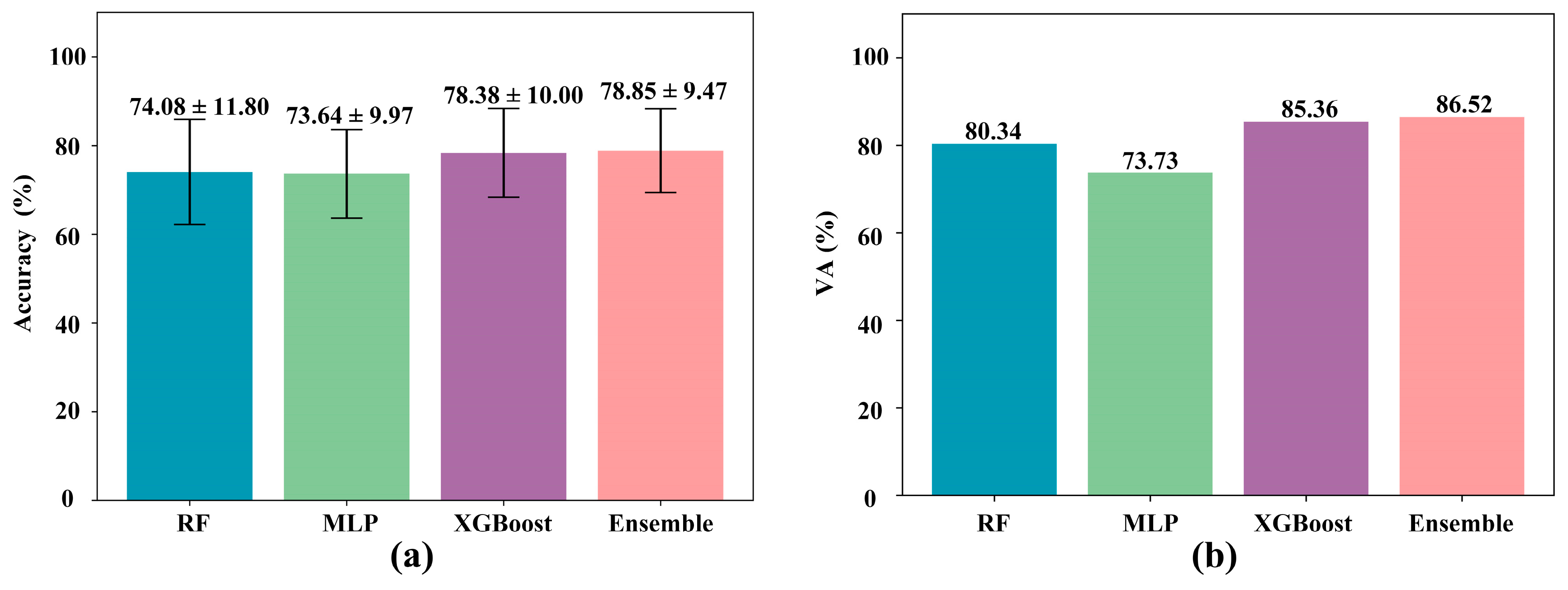
| LOPV | RF | 74.08 ± 11.80 | 75.04 ± 12.01 | 70.19 ± 13.60 | 80.34 |
| MLP | 73.64 ± 9.97 | 73.71 ± 10.88 | 69.37 ± 12.36 | 73.73 | |
| XGBoost | 78.38 ± 10.00 | 78.01 ± 10.64 | 74.77 ± 11.77 | 85.36 | |
| Ensemble | 78.85 ± 9.47 | 78.73 ± 9.840 | 75.43 ± 11.34 | 86.52 |
| Facial Region Selection | Metric (%) | ||||||
|---|---|---|---|---|---|---|---|
| Eye | Mouth | Head | Gaze | Accuracy | Precision | Recall | VA |
| √ | 43.34 ± 11.29 | 44.74 ± 12.79 | 38.13 ± 11.71 | 43.82 | |||
| √ | 54.95 ± 11.66 | 54.13 ± 13.51 | 49.96 ± 13.87 | 57.30 | |||
| √ | √ | 56.93 ± 12.00 | 54.30 ± 13.67 | 51.04 ± 13.21 | 60.67 | ||
| √ | 41.10 ± 11.83 | 75.65 ± 8.54 | 26.37 ± 13.82 | 38.20 | |||
| √ | √ | 47.68 ± 12.98 | 48.27 ± 15.04 | 41.68 ± 14.95 | 50.56 | ||
| √ | √ | 57.47 ± 12.17 | 56.04 ± 14.08 | 51.90 ± 14.96 | 62.36 | ||
| √ | √ | √ | 60.47 ± 12.53 | 57.57 ± 15.10 | 54.61 ± 14.82 | 63.48 | |
| √ | 70.51 ± 11.19 | 69.40 ± 13.03 | 65.74 ± 12.77 | 74.16 | |||
| √ | √ | 72.93 ± 10.56 | 71.85 ± 11.51 | 68.38 ± 11.71 | 78.09 | ||
| √ | √ | 74.90 ± 10.02 | 75.17 ± 11.10 | 70.72 ± 12.27 | 79.21 | ||
| √ | √ | √ | 76.58 ± 10.12 | 76.49 ± 9.93 | 72.54 ± 12.22 | 82.58 | |
| √ | √ | 73.35 ± 10.24 | 72.52 ± 11.60 | 69.11 ± 11.68 | 79.78 | ||
| √ | √ | √ | 75.74 ± 10.06 | 74.85 ± 11.07 | 71.60 ± 11.75 | 82.58 | |
| √ | √ | √ | 77.67 ± 9.44 | 77.62 ± 10.47 | 74.01 ± 11.57 | 85.39 | |
| √ | √ | √ | √ | 78.85 ± 9.47 | 78.73 ± 9.84 | 75.43 ± 11.34 | 86.52 |
Disclaimer/Publisher’s Note: The statements, opinions and data contained in all publications are solely those of the individual author(s) and contributor(s) and not of MDPI and/or the editor(s). MDPI and/or the editor(s) disclaim responsibility for any injury to people or property resulting from any ideas, methods, instructions or products referred to in the content. |
© 2025 by the authors. Licensee MDPI, Basel, Switzerland. This article is an open access article distributed under the terms and conditions of the Creative Commons Attribution (CC BY) license (https://creativecommons.org/licenses/by/4.0/).
Share and Cite
Xu, C.; Huang, W.; Liu, J.; Li, L. Detecting Driver Drowsiness Using Hybrid Facial Features and Ensemble Learning. Information 2025, 16, 294. https://doi.org/10.3390/info16040294
Xu C, Huang W, Liu J, Li L. Detecting Driver Drowsiness Using Hybrid Facial Features and Ensemble Learning. Information. 2025; 16(4):294. https://doi.org/10.3390/info16040294
Chicago/Turabian StyleXu, Changbiao, Wenhao Huang, Jiao Liu, and Lang Li. 2025. "Detecting Driver Drowsiness Using Hybrid Facial Features and Ensemble Learning" Information 16, no. 4: 294. https://doi.org/10.3390/info16040294
APA StyleXu, C., Huang, W., Liu, J., & Li, L. (2025). Detecting Driver Drowsiness Using Hybrid Facial Features and Ensemble Learning. Information, 16(4), 294. https://doi.org/10.3390/info16040294