SPARC: A Human-in-the-Loop Framework for Learning and Explaining Spatial Concepts

Abstract

In this article, we introduce a novel framework for learning spatial concepts within a human-in-the-loop (HITL) context, highlighting the critical role of explainability in AI systems. By incorporating human feedback, the approach enhances the learning process, making it particularly suitable for applications where user trust and interpretability are essential, such as AiTR. Namely, we introduce a new parametric similarity measure for spatial relations expressed as histograms of forces (HoFs). Next, a spatial concept is represented as a spatially attributed graph and HoF bundles. Last, a process is outlined for utilizing this structure to make decisions and learn from human feedback. The framework’s robustness is demonstrated through examples with diverse user types, showcasing how varying feedback strategies influence learning efficiency, accuracy, and ability to tailor the system to a particular user. Overall, this framework represents a promising step toward human-centered AI systems capable of understanding complex spatial relationships while offering transparent insights into their reasoning processes.

1. Introduction

Understanding our world relies on the ability to describe the relative spatial relationships of objects. This spatial knowledge is so crucial that Gardner’s Theory of Multiple Intelligences includes spatial intelligence as one of the eight fundamental types of intelligence [1]. Regarding Artificial Intelligence (AI) tasks, spatial intelligence is necessary for signal-to-text reasoning [2,3], computer vision [4], scene understanding [5,6,7], robot navigation [8], and human–robot interaction [9]. However, integrating spatial understanding into AI systems remains a significant challenge. Therefore, we need new AI solutions that can efficiently encode, analyze, and report spatial understanding.

Perhaps the most straightforward aspect of spatial intelligence is a single relation between two objects. In prior work, these spatial relations were calculated, compared, linguistically summarized, and used for decision-making tasks. However, many problems exist where a single spatial relation cannot sufficiently describe a task. For example, applying parts-based recognition to an airplane may consist of a fuselage, wings, and tail wings. Here, the spatial relations between these components could be used to identify a valid configuration for a plane. Furthermore, the spatial complexity would only grow if the task became more granular with the number of parts. This paper will refer to these sets of interrelated spatial relations as spatial concepts.

Many AI solutions for identifying parts-based concepts rely on the implicit learning of spatial relations. As such, it disregards the utility of being able to produce explicit information to help users build trust in the system. This capacity to provide explanations and ultimately establish user trust becomes even more critical in domains with limited data and/or where help from a human expert is vital. To use the airplane example again, with an explicit spatial learning approach, explanations such as “this image does not contain a private airplane because the wings of this plane are high relative to the fuselage. This plane is most likely a passenger plane” can be used. These types of explanations can help a human understand the AI’s reasoning and provide feedback to improve both the AI and human–AI paired performance.

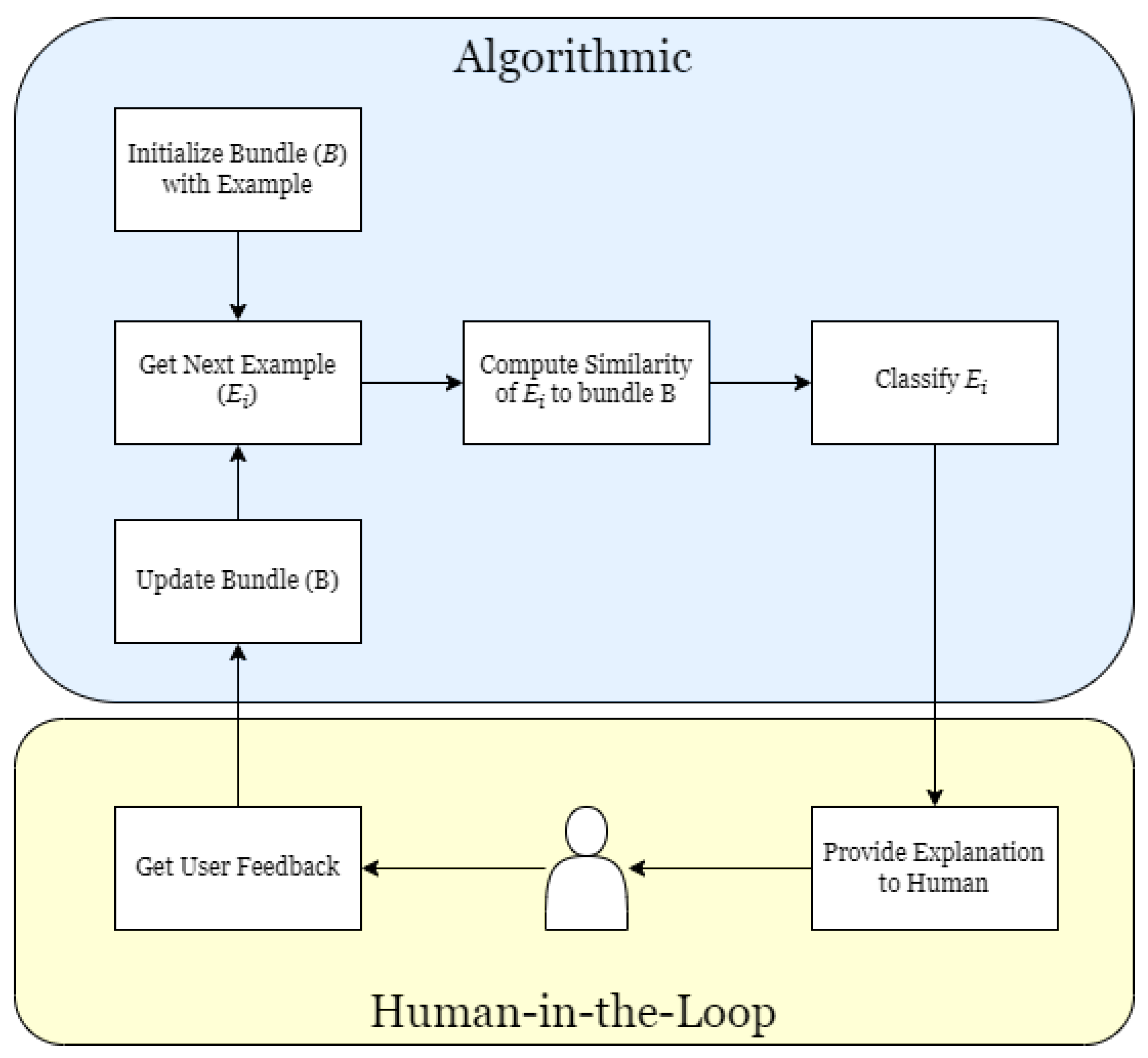
In this article, we introduce SPARC, a framework for Spatial Prototype Attributed Relational Concept Learning. A graphical outline is shown in Figure 1. Our contributions include a parametric measure for assessing the similarity between spatial relations encoded as histograms of forces, a data structure representation for spatial concepts and a human-influenced process for learning concepts. While this process can be used to learn spatial concepts across users, it can also be tailored to a specific user to account for the inherent relative nature of spatial intelligence. This work serves as an initial controlled step to introduce SPARC, demonstrating the feasibility of the approach using synthetic examples. A comprehensive human factors study will be explored in future research.

To further motivate our work and illustrate its practical relevance, we emphasize that the SPARC framework is designed not merely as a theoretical exercise but as a tool to solve tangible, real-world problems. For instance, in applications such as object detection and scene understanding, a spatial, parts-based reasoning approach is essential for accurately interpreting complex scenes. Similarly, in medical imaging and anatomical analysis, our method can support tasks ranging from the diagnosis of organ and tissue abnormalities to assessing the pose or gait of humans and animals. Furthermore, the framework holds promise for indexing and retrieval applications where a user-provided example guides the search for similar items or the closest match.

Our approach, unlike traditional black-box, data-driven models that rely on vast amounts of data, is tailored for niche, data-limited domains. It emphasizes transparency by explicitly revealing its internal decision-making processes, adapting to different user interactions, and providing detailed explanations, qualities that can enhance the role of a human analyst in specialized settings such as geospatial analysis, including risk assessment of flood-prone areas [10].

The remainder of this article is organized as follows: Section 2 reviews current techniques for learning and evaluating spatial concepts. Section 3 details the implementation of SPARC. Section 4 applies the framework to two synthetic examples. Finally, Section 5 summarizes findings, draws conclusions, and outlines directions for future research.

2. Background

The framework eluded to in the Introduction section intersects multiple domains, from human in the loop to large language models, concept learning, and spatial relations. In this section, we review prior work in each of these areas to contextualize our contributions.

Human-in-the-loop (HITL) systems incorporate human expertise into machine learning processes to enhance performance, especially in complex tasks where a person’s expert knowledge and intuition are valuable. HITL approaches have been effectively employed across various domains, such as active learning [11], where models interactively query users to label uncertain instances, improving learning efficiency. In recommender systems, user feedback is used to refine recommendations for personalization [12]. SPARC leverages these HITL principles to learn explicit spatial concepts, provide explanations, and build user trust through transparent interactions.

Large language models (LLMs) have shown remarkable proficiency in natural language understanding and generation. While explainable AI and its effect on human perception is a much broader AI topic [13], Yamada et al. [14] recently explored our ability to evaluate spatial understanding for LLMs. They concluded that while LLMs have achieved some measurable success in addressing spatial intelligence through implicit learning, there remains significant room for improvement. To date, no clear understanding of how LLMs compute, compare, or reason about spatial relations exists. As such, attempts to describe the spatial behavior of an LLM is a post hoc endeavor, which is essentially analyzing a black-box’s behavior versus the reasoning process. In contrast, herein, we introduce an explicit framework for representing, comparing, and utilizing spatial knowledge for HITL applications, focusing primarily on domains where data are limited rather than more abundant domains. An interesting line of future work could be exploring the integration of our methodologies into LLMs, enhancing their ability to compute, compare, and explain spatial concepts.

Concept learning involves inferring a general concept or rule from specific examples, a core challenge in machine learning. Traditional methods include symbolic learning algorithms like decision trees and rule induction [15], while recent approaches leverage deep learning to capture complex patterns [16]. In the context of spatial reasoning, concept learning has been applied to recognize patterns and configurations, often using relational learning approaches [17]. Active learning techniques allow models to efficiently learn concepts by querying informative examples [11]. Our framework contributes to this area by explicitly representing spatial concepts using attributed relational graphs and learning them through human-guided interactions, enhancing interpretability and adaptability.

In order to support interactions in the real world, account must be taken of the relationships between objects in space. These relationships should involve both the relationships of objects to each other as well as to a person. Such relationships are known as spatial relations [18,19]. For spatial relations, topological, directional, and distance relations are most commonly utilized.

To determine a spatial relation, a reference object must be specified to determine the relationship to an object of interest [20]. One common approach uses a bounding box around the objects, especially if the reference object is much larger than the one of interest. For directional relations, qualitative assessments are used to specify how a region or object is positioned relative to others [21]. In order to provide descriptions of these assessments, qualitative (symbolic) expressions that are not quantitative (numerical) can be used. Some examples of such directional relations could be the following: in front of, above, under, etc. These sorts of relations can be used in formulating queries particularly as they constrain and specify objects and regions’ positions relative to each other. For example, a query might be “Determine all regions or objects x, y, z so that x is front of y and y is above z”.

Furthermore, directional relations can be specified as either internal or external directional relations. So, internal directional relations determine where an object is positioned inside a region used as a reference. Some examples of this would be “left”, “on the back”, and “aft”. However, an external relation specifies where the object is located outside the reference objects. Such as “on the right of”, “behind”, “in front of”, and “abeam”. Lastly, distance relations specify the distance: how far from a reference region is an object of interest located. For example, “near”, “far”, “close”, and “in the vicinity”.

For Geographical Information Systems (GISs) [22], spatial relations are considered in the computation and analysis of geographic features. Specifically, this means how they are to be considered in relation to each other. Users of the GIS are then able to identify and query and specify their applications using especially topological relationships relative to spatial objects in the database [23]. Some of the relationships can be specified by terms such as overlaps, intersects, contains, and other similar specifications. Their determination uses the coordinates of any two or more objects being considered. So, this generates descriptions of how the geographic objects are, respectively, situated in their context [24]. For a GIS, this is a core function which allows a number of approaches to spatial analysis and the manipulation of data [25].

Understanding spatial relations is fundamental in computer vision [4], robotics [9], and GISs [26]. Classical approaches include qualitative spatial reasoning frameworks like Region Connection Calculus (RCC) [27] and the nine-intersection model [28], which provide symbolic representations of spatial relationships such as adjacency and containment. Quantitative methods, such as the histogram of forces (HoFs) [29], model spatial relations using the fuzzy set theory to capture directional and distance relationships while considering object shape and size. Recent advances involve deep learning models that implicitly learn spatial relations from data, such as spatial transformer networks [30] and graph neural networks for scene understanding [31]. However, the quality of these solutions is a function of data; only relatively simple spatial relationships have been demonstrated, and it is unclear how a spatial explanation would be produced for a user. Our work builds upon the HoF method for encoding spatial relations. It extends it by incorporating human feedback and applying it to a learning process, aiming to develop transparent and adaptable models that align with human spatial reasoning.

It is important to articulate the following concept. While existing approaches provide a foundation for explicitly representing spatial relationships or implicitly learning spatial relations from data, neither is inherently equipped to address a critical challenge: the relativity of spatial concepts. Spatial understanding often varies between individuals; for example, the interpretation of a phrase like “to the left of” can differ significantly, especially as the complexity of objects and their configurations increases. Moreover, how users reason about and utilize this spatial information also varies. This distinction is particularly relevant in applications where the goal is to create systems that emulate a specific user’s spatial intelligence, such as in the case of an analyst. In data-limited domains with specialized tasks, achieving such machine–human alignment requires minimizing user workload and learning from as few examples as possible. In summary, while existing works contribute to spatial intelligence, they are not designed to address the nuanced and relative challenges described here.

Histogram of Forces

One of the main goals of this paper is to develop a learning algorithm for spatial concepts that can be tailored to different users on a relatively low number of examples. Achieving this requires an effective representation of how objects are positioned relative to each other. Several methods have been proposed to describe object locations in images. Among these, the HoF, introduced by Matsakis [29], serves as a mechanism for encoding relative positions between objects rather than directly producing spatial relations. It can be computed in $O\left(N\log N\right)$, where N is the number of pixels in the image. It employs the fuzzy set theory to model the relative positions of objects while considering aspects such as their shape and size. It has been further extended into 3-D [32]. The HoFs can easily be used to draw linguistic explanations of the relative positions [33].

The HoF is particularly useful for evaluating directional spatial relations between objects. It measures the degree of “force” exerted by one object at a specific angle $\theta$ relative to another object. This force is assessed at every angle, with the x-axis of the HoF representing the angles and the y-axis showing the corresponding force intensity. One of the key advantages of the HoF is its affine invariance [34], allowing it to provide robust similarity measures regardless of rotation, translation, or scaling of objects. The HoF can accurately represent simple directional information such as “A is to the left of B” and more complex information such as “A surrounds B”. Importantly, the HoF does not directly define spatial relations (e.g., “A is to the left of B”), but rather encodes a structured representation of relative position that can be leveraged for multiple purposes, one of which is spatial relation extraction.

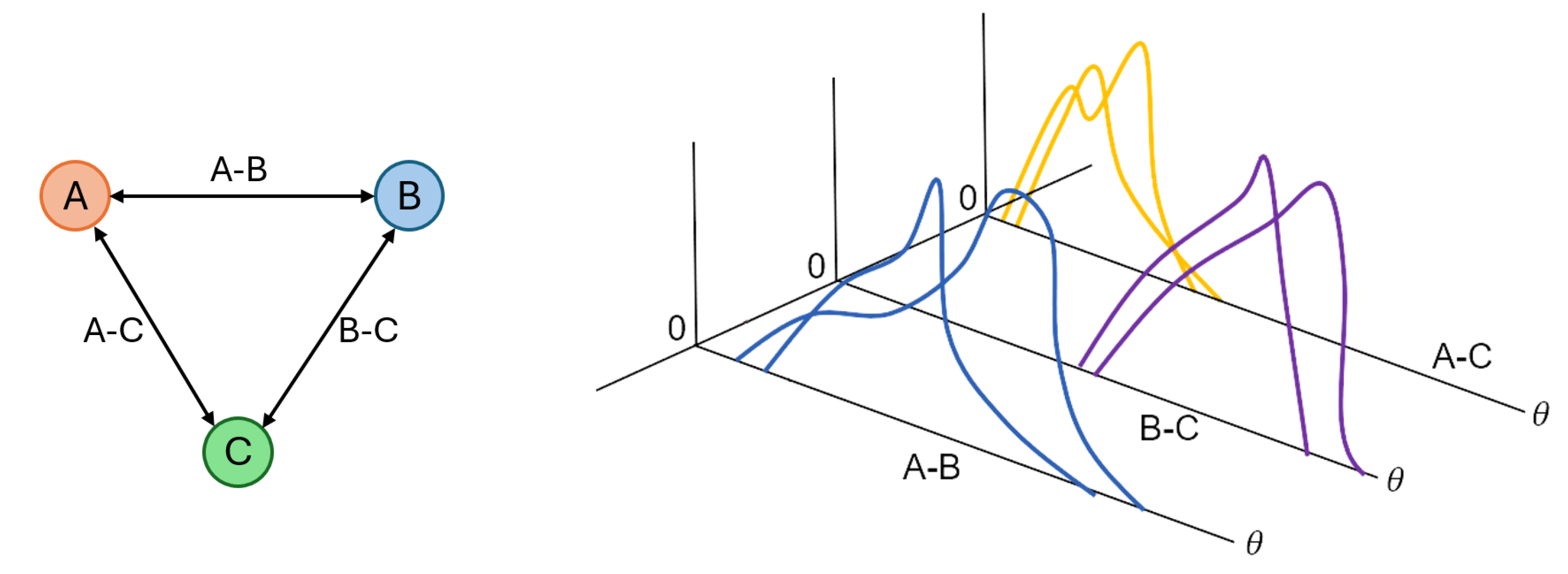
The histogram of gravitational forces (HoGFs), which is used in the remainder of the paper, is an extension of the HoF that varies the magnitude of the histogram according to the inverse square of the distances between the two objects. This modification allows the HoF to be able to additionally encode distance information. Figure 2 provides an example of how spatial relations can be encoded utilizing the HoGF. In Figure 2a, the black reference object is compared to a circle located in five different locations (shown by colors). Each square–circle combination results in a HoF, shown in Figure 2b. In Figure 2b, the x-axis is the angle, which can vary between 0 and 360 degrees. The y-axis value is the relative force magnitude. The reader can see that as objects change in relative angle, the HoF shifts in x, and as they vary in distance, the HoF changes in magnitude. As objects change in relative angle, the HoF shifts in x, and as they vary in distance, the HoF changes in magnitude—demonstrating how the HoGF provides a rich, adaptable encoding of relative position, which can be used for, but is not limited to, spatial relation modeling.

3. Methodology

3.1. Spatially Attributed Relation Graph (SARG)

As already discussed, many modern approaches, e.g., recurrent neural networks and LLMs, go the route of implicit spatial concept learning. Herein, our approach, SPARC, is explicit. Beyond the choice of how to model spatial relations, the next choice is how to store examples into a spatial concept. The structure chosen to represent spatial concepts was the attributed relation graph (ARG). The ARG, in the case of this framework, is mainly used to store spatial information, so we refer to it as a SARG. The SARG, G, is where each vertex is representative of a single object. Currently, G is a complete directed graph with ${\displaystyle \frac{n!(n-1)!}{2}}$ edges, E. Given this structure, the storage complexity of the SARG would be $O(n!m)$, where n is the number of objects in the spatial concept and m is the number of examples stored in the spatial concept. The SARG was chosen for three main reasons: its flexibility, extensibility, and explainability. The information that the SARG can store is flexible for the application being applied. The data stored in a SARG come in two broad types. The SARG can store attributes about a specific object as node attributes. These node attributes could be shape, texture, color, or geolocation. The SARG can also store information about the relationships between objects at attributes in the edges.

Although simple, examples can be highly illustrative. In the Introduction, we discussed vehicle recognition, such as identifying parts of an airplane. Another example of a spatial concept is the human face, where the components—eyes, nose, mouth, and other features—constitute the parts. A further example relevant to remote sensing involves geospatial concepts, such as a baseball diamond with parts like bases and stands. These examples demonstrate how different spatial concepts can be represented as a SARG.

It is also crucial to distinguish between different types of spatial concepts. Some, like those mentioned above, are relatively closed sets with well-defined parts. In contrast, others are more open-ended. Consider, for instance, a construction site. Such a concept can be highly complex and not easily captured through a fixed set of rules or examples. Nevertheless, even an open-set concept like this can still be represented and stored as a SARG by incorporating relevant examples.

Adding new objects to a spatial concept encoded as a SARG is relatively trivial. For example, a new node is created, and edges are established for all relevant existing nodes. In SPARC, these explicitly stored attributes allow transparent explanations of the learning algorithm’s decisions to be returned to a human user. For example, they provide the basis to provide a user with an explanation such as “the current example is not part of the spatial concept because object one and object two are too close together” from a single attribute if that attribute was dissimilar between the example and the learned concept. These explanations will allow a user to understand the reasonings that the learning algorithm used when identifying examples of the learned concept.

While a single value can be assigned per SARG attribute, herein, we store a collection of examples as a “bundle”. Later in this article, we outline a process for deciding what examples, HoFs to be specific, to add and how to use these examples for reasoning and explaining. It is important to note that spatial concepts are not as simple as a single example. For example, consider a task like facial sentiment analysis. A concept like a human face or “smiling” often does not have an exact spatial definition. These concepts are fuzzy. While an exemplar, or exemplars, might exist, it is important that a bundle exists per attribute in a SARG. Thus, in the current article, we use a SARG to represent a spatial concept; attributes are bundles, and individual examples in a bundle have an underlying degree of truth. Figure 3 is a visualization of a bundle for a concept with three objects and two examples.

3.2. Similarity Measure

Now that we have selected a data structure to represent spatial concepts, the question becomes how to compare examples. First, we must determine how we should compare the HoFs of the examples that make up the SARG with a newly presented example. We started by using similarity measures from the HoF community, namely the Jaccard index and cross-correlation. However, when performing initial experiments, we found that these similarity measures do not align well with human understanding. For example, while the Jaccard index is relatively forgiving regarding the closeness of objects, it is overly sensitive to changes in their relative angles. As it treats the histogram of forces as a collection of discrete bins, even a slight shift in relative angle can move an object’s representation from one bin to another. This bin-to-bin transition causes a dramatic drop in the overlap between histograms, thus a lower Jaccard index similarity, even when a human would still perceive the spatial configuration as essentially the same. In summary, these human alignment issues led us to explore the creation of a new way to measure proximity between spatial relations. We selected the Earth Mover’s Distance (EMD) because it is easily parameterized, allowing it to be adjusted to match a large range of spatial concepts. In the remainder of this subsection, we outline a new similarity method based on the EMD. In the remainder of this subsection, we outline a new similarity method based on the Earth Mover’s Distance (EMD).

The EMD could be defined as follows. Let h be a (1-D) histogram of length $L_1$, $h_i\in {\mathfrak{R}}^{+}$ and $1\le i\le L_1$, and let g be a second histogram of length $L_2$ and $g_j\in {\mathfrak{R}}^{+}$. The EMD defines the relative distance between a set of two HoFs: h and g. The goal of the EMD is to find a flow $F=\left[f_{ij}\right]$, where $F^{\ast }$ is the flow between $h_i$ and $g_j$, that minimizes the following equation.

$$WORK(h,g,F,D)=\sum _{i=1}^{L_1}\sum _{j=1}^{L_2}{d}_{ij}{f}_{ij},$$

(1)

subject to the constraints

$$f_{ij},1\le i\le L_1,1\le j\le L_2,$$

(2a)

$$\sum _{j=1}^{L_2}{f}_{ij},\le h_{i}1\le i\le L_1,$$

(2b)

$$\sum _{i=1}^{L_1}{f}_{ij},\le b_{j}1\le i\le L_1,$$

(2c)

$$\sum _{i=1}^{L_1}\sum _{j=1}^{L_2}{f}_{ij}=min(\sum _{i=1}^{L_2}{h}_i,\sum _{j=1}^{L_1}{b}_j),$$

(2d)

where $D=\left[d_{ij}\right]$ is the ground distance matrix. $d_{ij}$ is set to be the pair-wise distance between $h_i$ and $g_j$. The EMD is classically visualized as treating two histograms as though they are two piles of earth or sand, and the goal is to compute the total amount of work required to transform one into the other. The ground distance matrix is the distance from one location of earth (bin) to another (bin). Once the optimal flow, $F^{\ast }$, is found, the EMD is calculated as

$$\mathrm{EMD}(h,g,D)={\displaystyle \frac{{\sum }_{i=1}^{L_1}{\sum }_{j=1}^{L_2}{f}_{ij}^{\ast }{d}_{ij}}{{\sum }_{i=1}^{L_1}{\sum }_{j=1}^{L_2}{f}_{ij}^{\ast }}}.$$

(3)

While the EMD has been used in a number of applications, e.g., computer vision [35] and hyperspectral sensor processing [36], we explore it herein in a new setting to compare two spatial relations. In [37], we showed that well-known indices like the Jaccard, Dice, and KL divergence do not return comparable similarities to humans. In contrast, we explore this using a parametric metric based on the EMD, which allows for adjustable strictness in determining how closely an example must match to be considered part of a concept. This metric has additional parameters so that a human can tune the strictness of how close an example has to be in order to be part of the concept. This is achieved in two ways: via the ground distance and by an extended measure. Our new measure is

$$\begin{array}{cc}\hfill S\left(h,g\right)& ={{\displaystyle \frac{\min \left(v_h,v_g\right)}{\max \left(v_h,v_g\right)}}}^{\alpha }\hfill \\ & \times \left(1-EMD\left(h,g,{\displaystyle \frac{D}{\beta }}\right)\right)\hfill \end{array}$$

(4)

where $v_h$ and $v_g$ are the respective sums of h and g, and $\alpha$ and $\beta$ are user defined parameters. For our spatial relations setting, D is set such that it corresponds to the angular distance normalized so opposite values have a distance of one. In other words, two bins that are 180 degrees from each other will return a distance of 1. This decreases as the angular difference between two bins decreases till the distance is 0 for moving to the same bin. Mathematically, this can be expressed as follows:

$$D({\theta }_1,{\theta }_2)={\displaystyle \frac{|{\theta }_1-{\theta }_2|}{180}}$$

(5)

where ${\theta }_1$ and ${\theta }_2$ are the angular position of bins in degrees. The parameter $\alpha$ is used to control the overall sensitivity of the similarity measure. So, for a concept with strict spatial requirements, a larger $\alpha$ is more desirable. Conversely, for a concept that allows for more variability, a smaller $\alpha$ should be used. Parameter $\beta$ is used to control how sensitive our measure is to shifts in the relative angle between two objects. Specifically, $\beta$ is the number of bins that a histogram can shift before the distance measure ($\mathrm{EMD}(h,g,{\displaystyle \frac{D}{\beta }})$) is equal to 1, which would cause the similarity between the two histograms to be equal to 0. So, for example, if the HoFs consist of 180 bins ($2^{\circ }$ per bin) and a $\beta$ parameter of 10, then the EMD would produce values between 0 and 1 for changes in a relative angle less than ${20}^{\circ }$. These parameters help to allow for some intuitive control of the similarity measure by stating how sensitive the concept is to distance and angle. This similarity measure also has the nice feature that if the $\alpha$ is set to 1, then in cases where one histogram completely covers the second, the similarity value is equal to the Jaccard Similarity Index which in some contexts is also called the Intersection over Union (IoU).

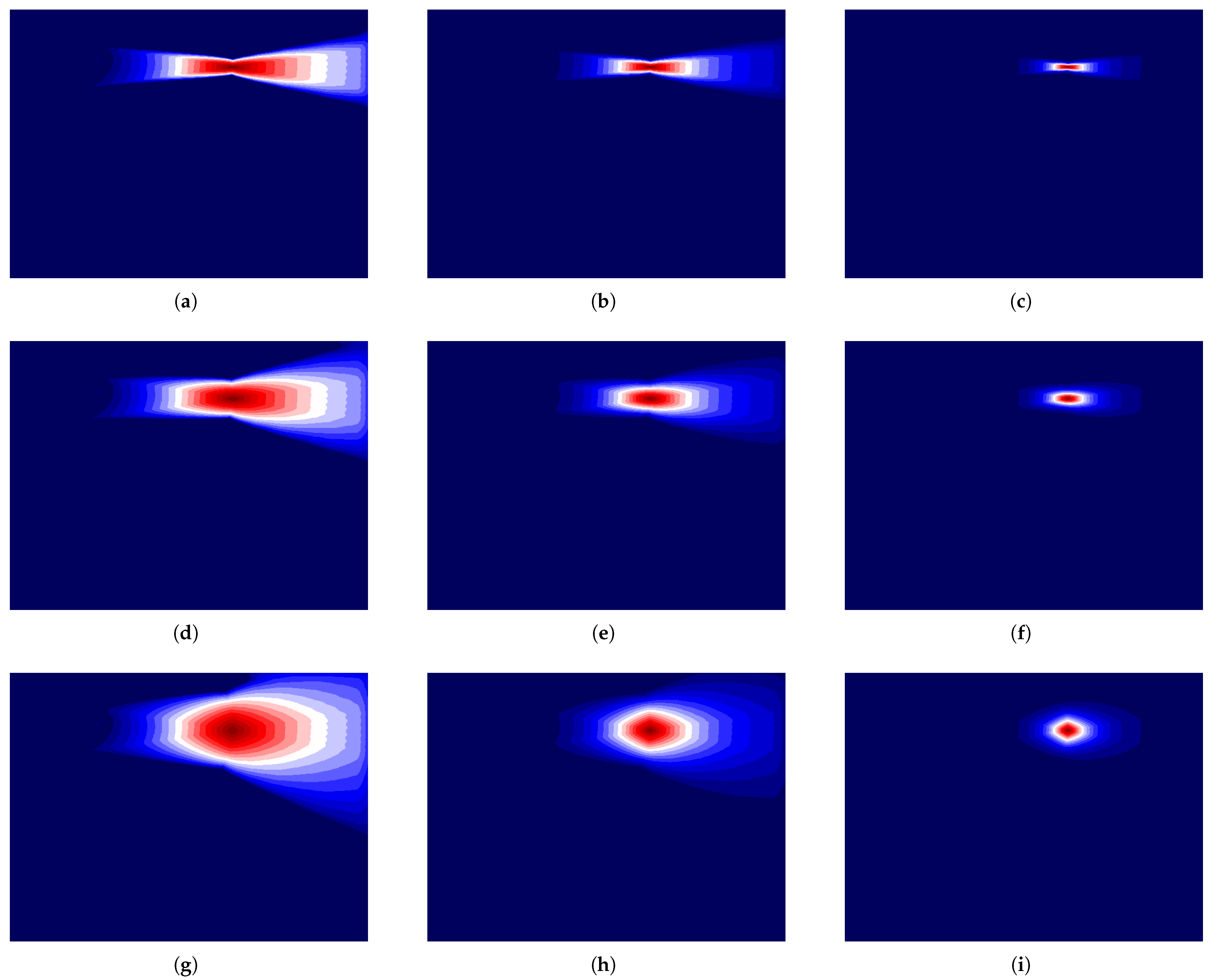
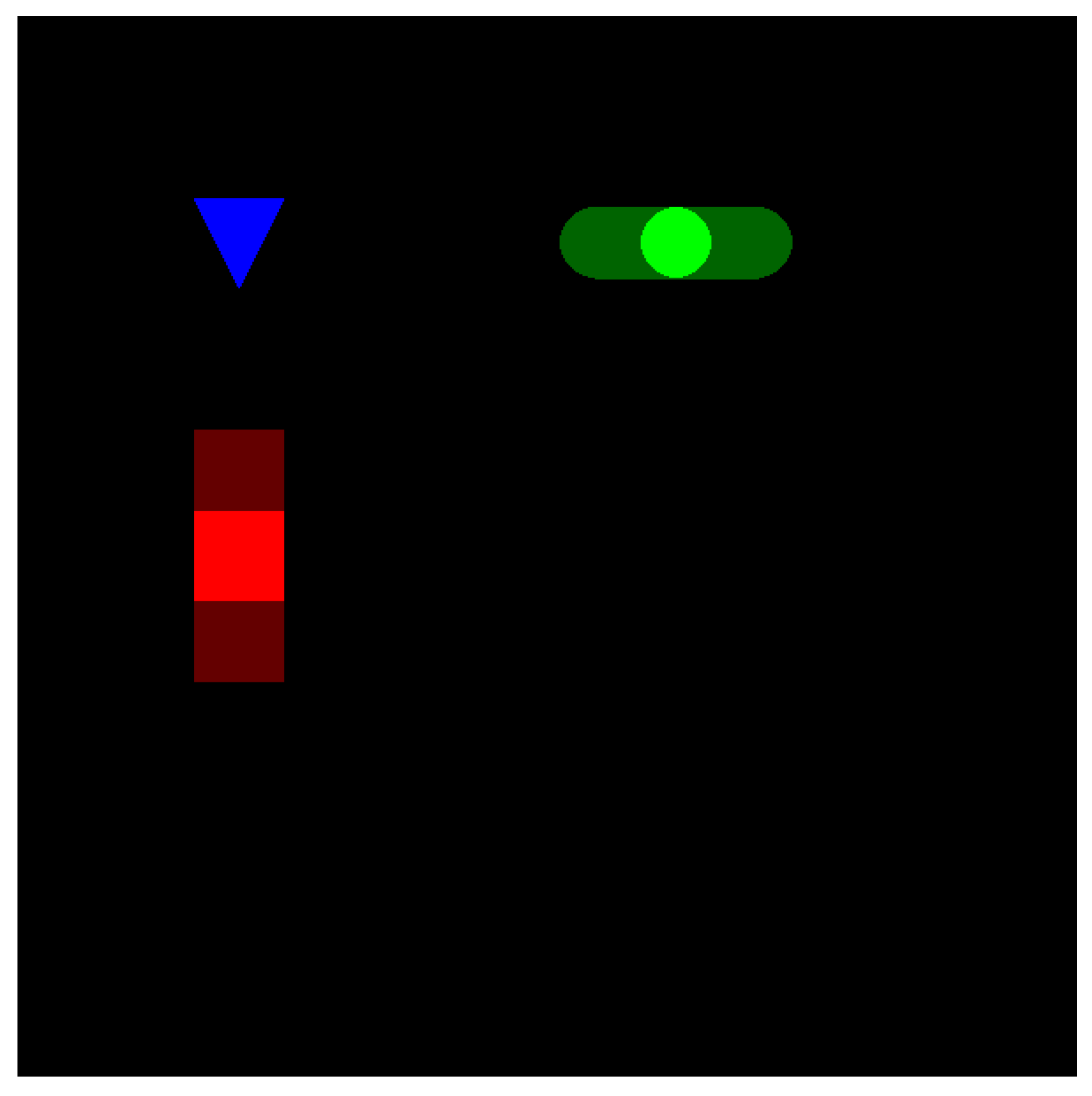
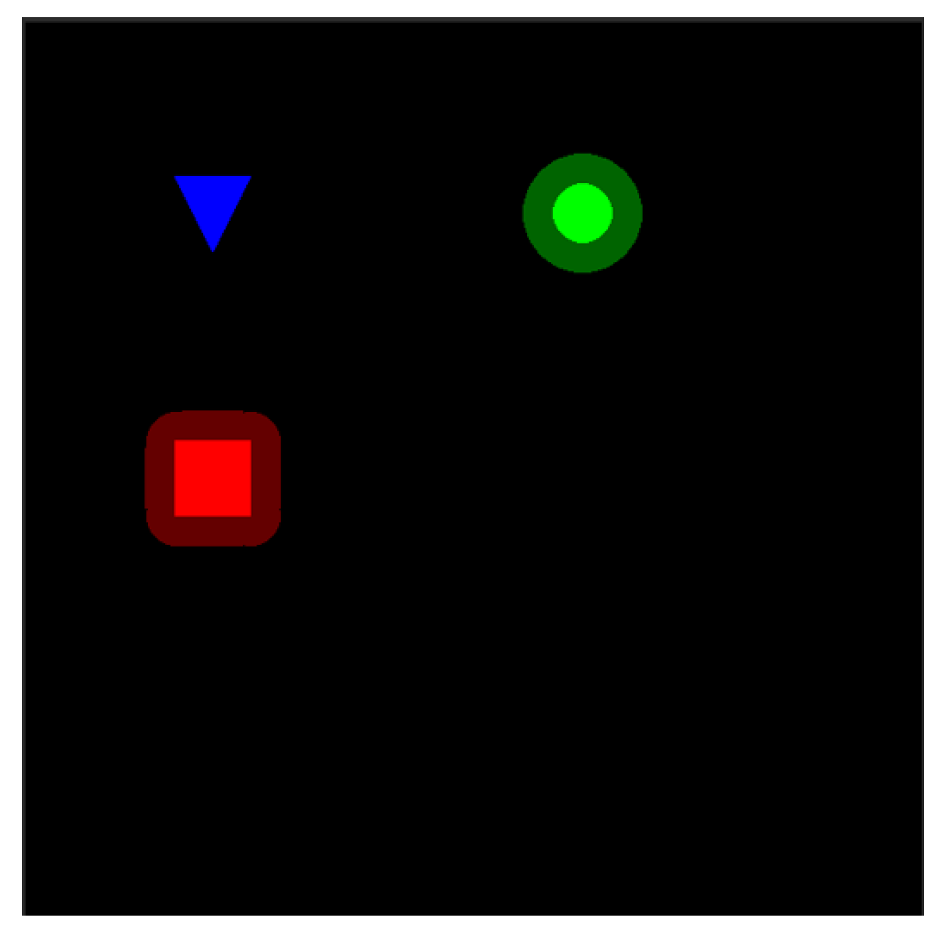
Now we will show visually the effect of the two parameters $\alpha$ and $\beta$. Figure 4 shows the initial positioning of the objects in an example concept. We are now going to examine how the similarity changes for moving the green circle in Figure 4 while under different parameter values for $\alpha$ and $\beta$ in Figure 5. For example, in Figure 5a, $\alpha =0.5$ and $\beta =4^{\circ }$. In this figure, each pixel represents the green circle being positioned at that pixel, and the intensity was set by the value of the similarity measure. The values of the similarity measure were then quantized to give a better view of what a decision boundary based on this similarity measure would look like. For the rest of Figure 5, a change in the row corresponds with an increase in the $\beta$ parameter of, respectively, $\left\{4^{\circ },{10}^{\circ },{20}^{\circ }\right\}$. Each column corresponds to an increase in the $\alpha$ parameter of, respectively, $\left\{0.5,1,{\displaystyle \frac{ln\left(0.5\right)}{ln\left(0.75\right)}}\right\}$. So, analyzing Figure 5 shows that increases in parameter $\beta$ can be thought of as a control on the effect that an angular change in the position of the objects causes. 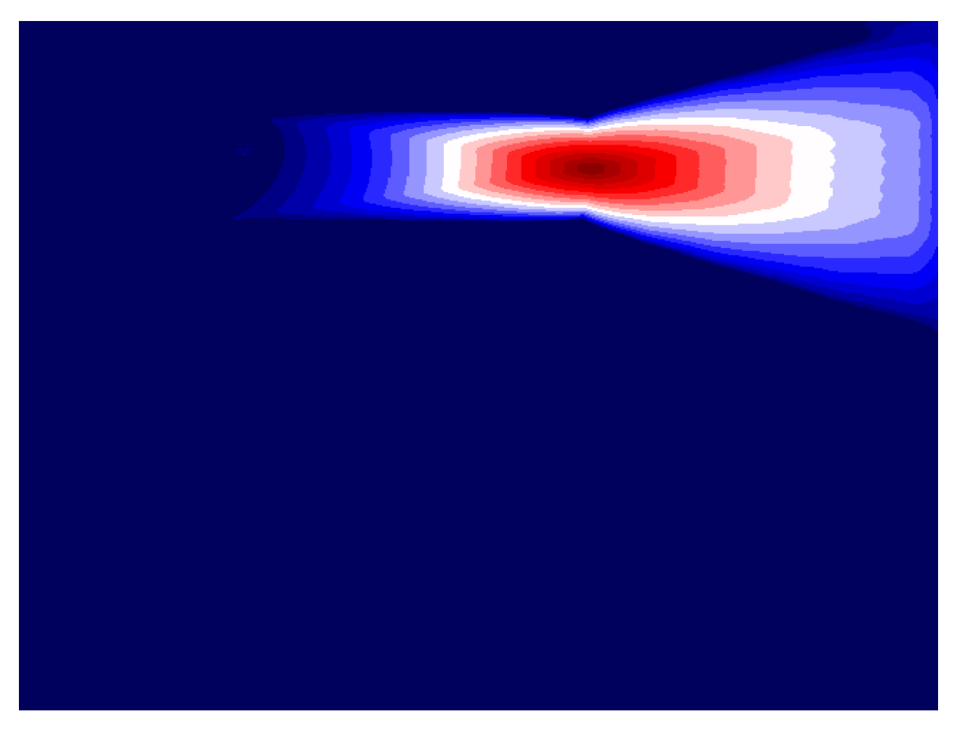Furthermore, an increase in $\alpha$ is a decrease in both the angular sensitivity and the effect moving the objects closer or farther away has on the similarity. As an added comparison, Figure 6 shows how the Jaccard Similarity Index performs on Figure 4. While it may be useful in some cases, it lacks the flexibility that this EMD approach can handle.

3.3. Sparc

Now that we have discussed how spatial concepts are stored and how to compare individual spatial relations, we can discuss the SPARC learning framework. The first step in this framework is to initialize the bundle. The bundle is a collection of all the examples the algorithm should consider when evaluating a new configuration of spatially located objects. Each bundle element consists of a SARG and a confidence value. This confidence value determines whether a given bundle element is an example of the concept or something outside of the concept. While not used explicitly in this paper, intermediate confidence values can be used in cases where the boundaries of the concept are fuzzy. One method of initializing the bundle is to select an example of the concept. In this paper, which uses examples where the bounds of the concept are clearly defined, the example used to initialize the bundle corresponds to the centroid of the bounds of the desired concept. Now that the bundle has been initialized, the learning process can begin.

The best way to describe the loop the process follows as part of the learning process is to start by showing the algorithm a new example. The first thing SPARC does with the new example is find the bundle element most similar to the example. The similarity between examples is conducted using the EMD to compare each spatial relation. Then, an aggregation method can combine the similarities into a single similarity, for example, of the bundle element. In this paper, we use a minimum as our aggregation method because this helps simplify the process conceptually and can be linguistically described as "the examples are only as similar as their weakest link." Once these similarities are computed, the algorithm’s next step is to classify the example as either part of the concept or outside. This classification can be performed using a threshold.

Now that we have analyzed the algorithm’s process of classifying examples, we could discuss updating our model by communicating with a human user. In order to receive feedback, the model needs to carry out three things. First, the model must inform the user of its decision on a specific example. There are a few different ways of passing this information back to a user, which are discussed in the next section.

Secondly, the user must have a way to provide feedback to the algorithm. The user can provide feedback in various ways. The first and most simplified is to allow the user to give feedback in the form of a binary decision, essentially telling the algorithm whether its decision on a specific example was right or wrong. This method is the most similar to how typical machine learning algorithms work on classification tasks and, as such, serves as a good baseline. The second method allows for a more fuzzy membership to be applied. With this, a user could inform the algorithm whether a given example is a good example, one close to the problem’s boundary, or if the example is outside the concept. The third method we have been working with is to have a user correct the algorithm and then provide a close example of a correct classification. This final method allows for both positive and negative feedback to be provided.

The final part of the user feedback component of the algorithm involves integrating the feedback into future decisions. This can be achieved by incorporating the current example into the bundle with a confidence level based on user feedback. Some methods of dealing with this are discussed at the beginning of Section 4.

3.4. Example

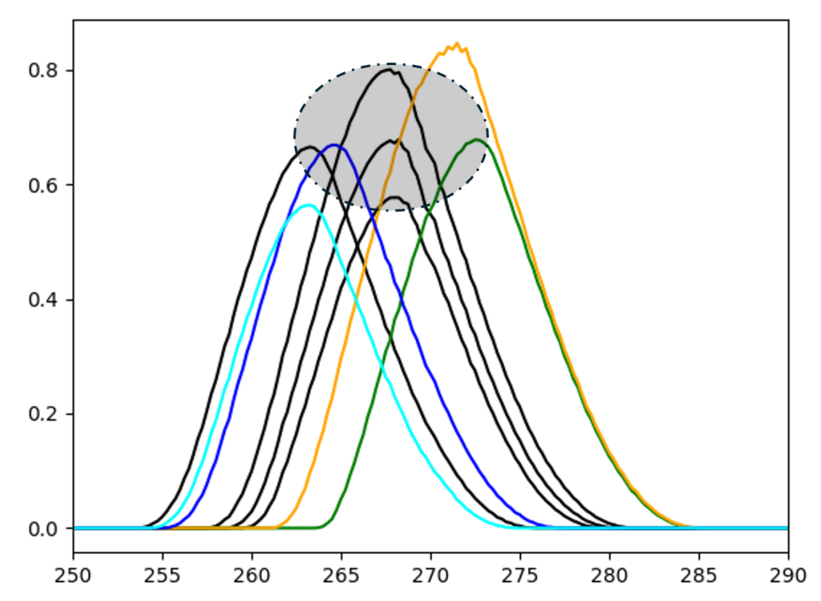
Let us consider a small spatial concept made up of two HoFs. This means that the SARG would have a single edge. Let the bundle be currently made up of four examples. The four spatial relations recorded in the bundle are the four black histograms shown in Figure 7. There is also a hypothetical human user who wants SPARC to learn a concept representing one of the objects being able to be placed in a circular region while the other object stays in the same position. This is indicated by the lightly shaded ellipse with a dashed outline overlaying the figure. A HoF is considered part of the concept if, and only if, its maximum value falls within this ellipse. Again, this ellipse is purely an illustrative mechanism for the reader to see a clearly defined zone of relative spatial relations. In general, we (e.g., SPARC) do not have access to such a truth, and it is likely the case that the user does not either, or the problem at hand would already be solved. Showing this acceptable zone is simply a mechanism to help the reader understand the proposed tool by assuming there is a clearly defined correct and incorrect answer to this task.

Figure 7 also includes several example HoFs—green, cyan, yellow, and blue—that are evaluated against the bundle. These examples illustrate how the algorithm classifies new data and how human feedback integrates into the learning process

The green HoF serves as the first example. The algorithm evaluates its similarity to each bundle element, using the minimum similarity among edges (in this case, only one edge is present). The highest similarity score among the bundle elements is 0.379, achieved with the center HoF. If the threshold for concept inclusion is set at 0.5, the algorithm would classify the green HoF as outside the concept. However, in this scenario, the hypothetical human user might decide that it does belong to the concept. When the human and algorithm disagree, one promising feedback method is to add the green HoF to the bundle as a positive instance of the concept, with a confidence score of 1.

For the cyan HoF, the bundle element with the highest similarity is the leftmost black HoF, with a similarity score of 0.782. The human user, however, considers the cyan HoF to be outside the concept. Consequently, one potential option for feedback is to add the cyan HoF to the bundle as a negative example with a confidence score of 0.

The yellow HoF represents a case where both the algorithm and the hypothetical human agree that it is outside the concept. The most similar bundle element is the topmost HoF, with a similarity of 0.497. Since the algorithm is already making the correct evaluation, feedback is not necessary, and the next example can be shown to the algorithm.

Last, the blue HoF is classified by the algorithm as part of the concept. The most similar bundle element is again the leftmost black HoF, with a similarity of 0.752. This aligns with the desired concept of the human user.

Although it may seem simple, this example, along with Figure 7, illustrates how the SPARC framework integrates algorithmic evaluation with human feedback in an iterative process to refine the learned spatial concept, ultimately enhancing classification performance and aligning more closely with user expectations.

3.5. Explanation

A key aspect of SPARC is its ability to generate explanation-structured interpretations of a model’s decision-making process for human analysts. These explanations are not merely outputs but structured, comprehensible rationales that bridge the AI’s internal mechanisms with human-recognizable concepts. In discussing explanations, transparency is equally critical—since not all explanations are equally valuable. Many provide little actionable insight, while others offer traceable chains of evidence for legal or accountability purposes, or even contribute to new domain knowledge. In the field of XAI, explanations vary in form, including statistical, graphical, or linguistic representations, at either a global or local scale. Additionally, some explanations are post hoc, derived from an AI’s observed behavior rather than its actual decision-making logic. Popular works include LIME [38], SHAP [39], and recent attempts to generate explanations from black-box LLMs, including whether self-generated explanations can be trusted [40]. In summary, SPARC prioritizes transparency by design, ensuring that its output is inherently interpretable. This structured approach enhances user trust, facilitates meaningful feedback, and fosters the development of collaborative, human-centered AI applications.

As part of the HITL process, it is crucial to effectively convey to the user what the model perceives as the underlying concept. There are various ways to accomplish this, but any chosen method will likely require distilling a bundle into one or a few representative examples to ensure human interpretability. In previous work, we proposed identifying the medoid of the bundle or a prototypical example by averaging each edge of the bundle of the SARG [41,42]. This approach enables the construction of clear, intuitive explanations of the learned concept. In [43], we showed one way to communicate this information through graphical visualizations based on the medoid or by leveraging deep learning.

Another method of communicating a bundle is through linguistic summarization of spatial relations. For example, in Figure 4, which is used in our first example, a potential linguistic description (generated by our algorithm in [3]) is as follows:

“The triangle is to the left of the circle and above the square.”

This natural language description is one way that an algorithm can give the user an overview of its understanding of the concept it is trying to learn. However, when the algorithm evaluates an example, the linguistic descriptions can again be used in a comparative analysis between the generated prototype and the example. Here, we could envision a situation where the response linguistic response is as follows:

“This is not an example of the concept because the circle is too far to the right.”

The key point is that our prior work has introduced several algorithms that are inherently tied to the data and model, rather than being post hoc or generative. These explanations span various forms, from graphical to linguistic, enabling users to better understand the model’s reasoning. By providing clear, interpretable insights, these explanations also facilitate more effective corrective feedback from users.

Since we have not yet introduced users into the process for the following examples or conducted human factors evaluations, we cannot definitively assess the degree to which these explanations enhance understanding or usability. However, it is essential to demonstrate that the system is capable of generating these explanations, laying the groundwork for future user-centered evaluations.

4. Examples

This section is two illustrative examples of how SPARC learns concepts. These examples are designed to showcase the practical implementation of SPARC. Analyzing specific cases gives a more lucid comprehension of how the framework and user types function in various scenarios. Each example has been carefully chosen to highlight a unique aspect or challenge associated with the framework, providing insight into its versatility and limitations. These examples demonstrate the principles discussed in the preceding sections, showing how the framework can be used to learn a spatial concept.

The following examples are not based on human factors testing. Instead, we utilize four different user types to test different types of interactions. These user types are simulated within the framework to analyze different potential human interactions. This is not a formal human factors study but rather an evaluation of the framework’s ability to adapt to different learning conditions. User 1 adds an example to the bundle every time an example is shown to it. User 2 is more relaxed and they only add examples if the algorithm incorrectly classifies the example. User 3 will, every time the algorithm incorrectly classifies an example, add that example to the bundle with the correct confidence and add a close example reflected across the concept’s boundary. This user helps the effect of a single data point from overcorrecting the algorithm’s decision boundary. User 4 is a hybrid approach combining User 2 and User 3. User 4 begins as a copy of User 3 and keeps track of how many mistakes have been made in the last 20 examples. This rolling accuracy is then evaluated, and once the rolling accuracy increases above a threshold, 80% used herein, it switches to user type 2 unless it drops below 75%, in which it switches back to User 3.

4.1. Example 1

In Experiment 1, we aim to evaluate SPARC’s ability to learn a well-defined spatial concept in a simple and controlled environment. Using basic shapes—a triangle, a square, and a circle—we eliminate the complexities introduced by more intricate designs or real-world data. It is important to understand the ability of a tool to work in such an ideal scenario and to observe how it behaves relative to different user types. This example is illustrated in Figure 8, where the slightly darker region highlights the location of the object within the predefined concept that the algorithm aims to learn. A test set was generated to compare with the learning region. For this initial example, the framework was applied to a dataset derived from Figure 8, running through 2000 iterations.

Figure 9 presents the accuracy results at each iteration during the learning process. The markers along the line indicate each time an element is added to the bundle. As shown, User 1 steadily improves its accuracy on the test set. After 2000 iterations, User 1 achieves the highest accuracy. The ability of User 1 to outperform other users, despite starting with a lower learning rate, demonstrates the robustness of its learned concept. In contrast, User 2 shows significantly lower accuracy as the number of examples increases compared to User 1. Additionally, there are substantial fluctuations in accuracy for User 2, as it adds the fewest elements to the bundle. User 3 generally achieves better accuracy than Users 2 and 4 throughout most of the iterations, while still being surpassed by User 1. Finally, User 4’s performance falls between User 2 and User 3, which aligns with its hybrid characteristics.

Figure 10 offers a different perspective on the accuracy of learning the simulated spatial concept. It shows accuracy relative to the number of elements in the bundle. This provides an alternative way to interpret the results of Example 1. The chart illustrates the impact of adding individual examples to the bundle. It becomes evident that User 1 frequently adds examples that do not significantly improve accuracy. User 2 is somewhat more efficient, as it avoids adding examples that the algorithm already classifies correctly. The results for User 3 and User 4 indicate that including both positive and negative examples can yield better outcomes than the other users, even though this approach leads to two elements being added to the bundle whenever an error occurs.

4.2. Example 2

The second experiment increases the complexity by introducing a more relaxed spatial concept with less defined boundaries. The object configuration is, again, a triangle, a square, and a circle; however, in this case, the configuration bound has been modified, as shown in Figure 11. Since the concept bounds are more relaxed in this example, the algorithm was evaluated while actively learning 500 examples.

Figure 12 shows accuracy after each example iteration throughout learning. The markers along the line represent each time an element is added to the bundle. As seen here, User 1 steadily increases its test set accuracy. After 500 epochs, User 1 has the highest accuracy. The fact that User 1 can surpass all the other user types while starting with a lower learning rate highlights the robustness of its learned concept. User 2 has much lower accuracy as the number of examples shown increases relative to User 1. It is also possible to see a large number of fluctuations because this user adds the fewest number of elements to the bundle. User 3 has the best accuracy for most epochs before being barely surpassed at the very end. This means that it quickly learns a relatively good set of examples but struggles to add new ones later. Finally, User 4 has a result between User 2 and User 3, making sense as it is a hybrid of those users.

Figure 13 shows the accuracy of learning the simulated spatial concept in a slightly different light. Here, the results show a different way of examining the story of Example 2. In this chart, it is clear that User 1 adds many examples that are not that valuable to increasing the accuracy. User 2 is slightly better because it does not add examples that the algorithm already classifies correctly. User 3 and User 4 show that the impact of adding both a positive example and a negative example surpasses the results of the other two users, even though each time there is an error, two bundle elements are added instead of one.

5. Conclusions and Future Work

This article presented a novel framework for learning spatial concepts in a human-in-the-loop context. Furthermore, this approach is capable of generating a variety of explanation types to assist the user. Our approach integrates feedback to refine the learning process, making it particularly effective in domains where user trust and interpretability are critical, such as AiTR tasks. The framework demonstrated its robustness to various potential human interactions through the examples and user types explored, showing how different feedback strategies impact learning efficiency and accuracy. Furthermore, our experiments demonstrated that the proposed methods can be adapted to different users, though some users and user types may be more optimal than others. This makes our framework a promising step toward more human-centered AI systems capable of learning complex spatial relations while providing insights into their reasoning.

As outlined in our article, the first step involved using controlled synthetic examples, where establishing a known truth was essential for evaluating how the approach performs across different user types. In future work, we will extend our research to more complex spatial concepts that lack a definitive truth and vary based on user characteristics. This expansion will allow us to assess, through human factor metrics, which explanation types are most effective. However, our results revealed that different user types lead to distinct behaviors, raising an important question: what type of user is ideal for a given problem? While we demonstrated that the system can adapt to the user, it remains to be explored whether certain user types are preferable for specific tasks and whether AI can play a role in training users to improve performance. Ultimately, this research paves the way for developing human–AI systems that are more spatially aware, intuitive, and aligned with human cognitive processes.

This work represents an initial controlled study, demonstrating the feasibility of SPARC in learning spatial concepts through synthetic examples. Future research will involve a more rigorous human factors experiment, where real users interact with the system to assess its usability and effectiveness. Ultimately, this research paves the way for developing human–AI systems that are more spatially aware, intuitive, and aligned with human cognitive processes.