Constrained Gray-Box Identification of Electromechanical Systems Under Unfiltered Step-Response Data

Abstract

This paper presents a physically constrained grey-box identification framework for electromechanical systems, illustrated through the dynamics of brushed DC motors. The method estimates all electromechanical parameters by minimizing a normalized residual that combines current, velocity, and steady-state algebraic constraints under a current-limit condition. Classical approaches such as least-squares and black-box identification often lack physical interpretability and do not explicitly enforce steady-state consistency, making their estimates susceptible to nonphysical parameter drift. The proposed formulation incorporates these physical constraints within a Levenberg–Marquardt scheme with signal normalization, enabling the joint minimization of current and velocity errors. Validation was performed using step-response data from two DC motors under both synthetic and experimental conditions. When applied to unfiltered measurements, the method maintained steady-state relative errors below 1% and achieved low trajectory discrepancies, with NRMSE in velocity between 2.6 and 3.2% and NRMSE in current between 0.9 and 1.2% across both motors. Embedding physical and steady-state constraints directly into the cost function improves robustness and ensures physically consistent parameter estimates, even under high measurement noise and without filtering. The approach provides a general strategy for dynamic system identification under physical consistency requirements and is suitable for rapid calibration, diagnostic monitoring, and controller tuning in robotic and mechatronic applications.

1. Introduction

Accurate dynamic models of electromechanical actuators are essential in robotics, automation, and industrial drives because controller performance, stability, and safety margins depend directly on how well the model represents the real plant [1]. For this reason, parameter estimation based on time-domain experiments, including step responses, remains widely used, as such experiments provide practical and reliable motor models that reflect real operating conditions [2].

Parallel to these classical identification approaches, numerous studies have explored metaheuristic search methods such as particle swarm optimization, differential evolution, and genetic algorithms. These techniques can handle nonconvex cost functions but are often slower, more sensitive to hyperparameter tuning, and less predictable in practical performance [3].

Machine-learning-based parametric estimators have also been proposed to address nonlinearities in electromechanical systems, although they typically require large training datasets. In robotics, additional research has focused on the joint identification of inertial and motor parameters using PWM excitations and six-axis force/torque sensing along the kinematic chain [4].

An early example of constrained nonlinear fitting is provided by Wu [5], who estimated DC motor parameters from speed step responses. However, the method relied on filtered velocity measurements and omitted current data, reducing robustness and making the estimates susceptible to ill-conditioning or compensating parameter trade-offs. Later work, such as Hernández et al. [6], achieved accurate fits using the Steiglitz–McBride algorithm, but required digital filtering and did not enforce steady-state algebraic relationships. Recent studies have explored learning-based estimators, such as the neural-network parameter identification method of Siddiqi et al. [7], as well as rapid-control-prototyping approaches [8]; however, these methods are often validated only on synthetic or highly idealized datasets, limiting their applicability under realistic noise conditions.

Survey papers on motor modeling report comparisons between widely used identification strategies—including least squares (LS), particle swarm optimization (PSO), grey wolf optimizer (GWO), bat algorithm (BA), genetic algorithms (GAs), and neural networks. These reviews generally show that GWO achieves the smallest errors in open-loop settings, whereas LS remains the most computationally efficient method for closed-loop cases.

Overall, the literature reveals a persistent gap between physical interpretability and numerical performance. An identification method that is (i) explicitly grounded in an electromechanical model, (ii) robust to unfiltered measured signals, and (iii) consistent with steady-state relations and physically meaningful bounds is still lacking. Accurate modeling is also crucial for analyzing disturbances caused by noise, load variations, and environmental effects [9].

In this work, we address this gap with a grey-box identification method formulated as a simulation-in-the-loop constrained nonlinear optimization problem. The method preserves the physical meaning of the parameters, incorporates both steady-state and transient relationships, and enforces a current-limit condition to prevent nonphysical solutions. It estimates the five standard DC motor parameters directly from open-loop current and speed step responses and remains effective even with low-cost sensors and significant measurement noise, eliminating the need for digital filtering.

In summary, this paper makes the following contributions:

• We formulate a constrained grey-box identification framework for permanent-magnet DC motors that embeds electromechanical coupling, steady-state algebra, and a current-limit condition directly into the residual of a Levenberg–Marquardt optimizer, enabling joint estimation of the full parameter set $\{K,R,L,J,B\}$ from step-response data.
• We provide a detailed structural identifiability analysis based on normalized sensitivities and singular-value decomposition of a stacked sensitivity matrix, showing that all five parameters remain theoretically separable for two actuators with markedly different electrical and mechanical scales.
• We demonstrate that the proposed method achieves low trajectory errors on unfiltered experimental data from low-cost sensors, without any digital filtering or manual tuning, and we quantify parameter uncertainty using both Gauss–Newton covariance approximations and bootstrap-based dispersion measures.
• We empirically validate the robustness of the approach through Monte Carlo experiments over randomized initializations and by comparing against a standard least-squares baseline on the same raw datasets, highlighting the impact of physics-based constraints on both physical plausibility and NRMSE.

The remainder of the paper is organized as follows. Section 2 reviews related research. Section 3 presents the model, residual design, constraints, and optimization procedure. Section 4 reports results on simulated datasets and unfiltered measured datasets for two motors and discusses robustness and physical coherence. Section 5 summarizes the main findings and outlines potential directions for future work.

2. Related Work

To contextualize the contribution of this work,

Table 1. Positioning of the proposed method with respect to representative prior work.

Reference	Parameters Estimated	Data and Preprocessing	Physical Constraints	Main Focus vs. This Work
Jiménez–González et al. [10]	$R,L$ (no–load/DC tests); $J,B$ via RLS	No–load and DC tests; preprocessed signals	Limited (structural only)	Two–stage BLDC identification; our method handles full DC–motor coupling, uses raw step responses, and embeds physical constraints.
Chakraborty et al. [11]	$R,L,K,J,B$ (servo case)	Clean lab data; moderate filtering	Bounds and priors	Toolchain demonstration; our method targets unfiltered data with embedded physics.
Hadef et al. [12]; Hassan et al. [13]	Subsets or full via numerical ID	Preprocessed or well–conditioned data	Limited	Conventional identification; here we enforce steady–state/current limits and positivity.
Fazdi & Hsueh (review) [3]; Boudjemai et al. [14]	Varies (metaheuristics)	Often filtered; computationally heavy	Varies	Global search perspective; our focus is grey–box with lightweight constraints on unfiltered data.
Traversaro et al. [4]	Inertial + motor + friction	Robotics datasets; structured experiments	Structural	Robotic identification with friction; we emphasize DC–motor step responses with constraints and no filtering.
This work	$K,R,L,J,B$ jointly	Step responses; unfiltered velocity and current	Steady–state algebra, current bound, positivity	Full–set grey–box identification on unfiltered data; reduced preprocessing and strong physical consistency.

summarizes representative studies on DC motor parameter identification, highlighting their data requirements, physical constraints, and methodological focus.

Early studies on DC motor identification relied on analytical expressions derived from simplified physical models. Classical procedures estimate the main parameters from steady-state and no-load tests, avoiding mechanical loading, and similar test-based strategies remain common in recent DC and BLDC work [10]. Later, Wu [5] introduced a continuous-time nonlinear fitting approach to recover all parameters from speed step responses; however, this method depends on filtered velocity data and ignores current measurements, which limits robustness under realistic noise. Hernández et al. [6] applied the Steiglitz–McBride algorithm to discrete-time models and achieved adequate fits, but their approach also required digital filtering and did not enforce steady-state consistency. Although these analytical or semi-analytical techniques remain attractive for their simplicity, they typically treat electrical and mechanical subsystems separately and overlook frictional nonlinearities.

A second family of approaches introduced numerical optimization and grey–box modeling. Hadef and Mekideche [12] and Hassan et al. [13] employed inverse-problem formulations and iterative simulation fitting to estimate motor parameters from dynamic tests, while Chakraborty et al. [11] demonstrated a practical Simulink-based workflow for servo-drive parameter estimation using nonlinear least-squares optimization. These methods improved automation and reproducibility but still required clean or preprocessed data and offered limited guarantees regarding the physical admissibility of the estimated parameters.

With the growth of computational power, several authors have explored metaheuristic and hybrid search algorithms. Munciño et al. [15] investigated evolutionary and swarm-based techniques for DC motor parameter identification and demonstrated their flexibility in navigating nonconvex error surfaces. Boudjemai et al. [14] introduced an experimental MATLAB-based workflow for parameter fitting. Jesenik et al. [16] and Demirtas and Efe [17] combined differential evolution and particle swarm optimization within rapid-control-prototyping frameworks. Although these global-search methods can achieve robust convergence under noisy data, they remain computationally expensive, require multiple hyperparameters, and do not explicitly enforce algebraic or steady-state constraints. Alternative real-time estimation strategies, such as extended Kalman filters [18], have also been explored, but their performance depends strongly on model accuracy and sufficiently fast sampling.

More recently, learning-based estimators have also been explored. Siddiqi et al. [7] proposed a neural-network-based data-driven approach for estimating the parameters of permanent-magnet DC motors. Kim et al. [8] reported a rapid control-prototyping system for online identification. Traversaro et al. [4] extended parameter identification strategies to include inertial and frictional effects in robotic actuators, illustrating the advantages of modeling electromechanical coupling. Despite these advances, neural and metaheuristic approaches often rely on synthetic or filtered datasets and provide limited physical interpretability compared with grey-box formulations.

In summary, most previous studies either simplify the motor model to facilitate analytical computation or adopt black–box algorithms that disregard physical consistency. Very few works integrate both electrical and mechanical coupling while simultaneously enforcing steady–state algebra and physical constraints on unfiltered data. The present study bridges this gap by formulating a constrained grey–box identification scheme that unifies algebraic consistency, current–limit enforcement, and parameter positivity in a single physically coherent optimization process. This combination of physical interpretability, robustness to noise, and reduced preprocessing complexity defines the main methodological contribution of this work.

3. Materials and Methods

The identification procedure was designed to estimate the complete set of electromechanical parameters of brushed DC motors, namely the armature resistance R, inductance L, torque and back-emf constant K, viscous friction coefficient B, and total inertia J, by directly fitting the coupled electrical and mechanical model to measured step-response data of current and angular velocity. The study considered both real experiments on two DC motors (a Mavilor CML-050 and, for cross-validation, an RMCS2004 unit) and a small synthetic dataset generated from the same continuous-time model to provide a noise-free baseline for verification. This framework integrates experimental signal acquisition under controlled excitation with a continuous-time nonlinear optimization that enforces physical consistency and state-space constraints, bridging classical grey-box modeling with modern constrained estimation.

Experimental data were recorded using a small laboratory test bench, assembled similarly to the setup described by Hernández et al. [6]. The bench included a Mavilor CML-050 motor as the main unit and an RMCS2004 motor that was used only for cross-validation. A programmable power source supplied the voltage steps; in all cases, the maximum applied voltage was $10.5\mathrm{V}$. Current readings came from a precision shunt resistor connected to a differential amplifier, and the terminal voltage was taken directly from the motor leads. The shaft speed was obtained from a quadrature encoder attached to the axis. Data were captured using a PIC18F4550 microcontroller running at $1\mathrm{kHz}$ with 12-bit resolution and later sent to a computer through USB. Simple analog low-pass filters were added to the voltage and current channels to reduce aliasing. In practice, the signals contained typical laboratory noise, which was deliberately retained to evaluate how the algorithm performs on raw data. Each test consisted of applying a single voltage step from rest until the motor reached a steady state. All collected data were saved in CSV format for later processing.

In order to quantify the measurement quality of the unfiltered signals used in all experiments, the main noise characteristics of the acquisition chain are summarized here. The quadrature encoder provides an effective angular resolution of approximately $0.5$–$1.0\mathrm{rad}/\mathrm{s}$ per count at the typical operating speeds of the motors, which establishes the lower bound on velocity quantization. The current measurements are obtained through a precision shunt resistor followed by a differential amplifier with an effective bandwidth of several kilohertz, which is well above the electromechanical bandwidth of the actuators; the resulting RMS noise level, estimated from the pre-step segments, is approximately 1–2 LSB of the 12-bit converter. The applied voltage exhibits the expected PWM ripple from the laboratory supply, but this effect remains bounded and is captured directly in the raw data. These values characterize the disturbances present in the unfiltered signals. They justify treating encoder quantization, sensor noise, and PWM ripple as bounded perturbations within the identification framework.

In addition to real measurements, a synthetic dataset was generated from the dynamic model using nominal parameters from the Mavilor CML-050 datasheet. Two step voltages of 6 V and 8 V, each with a 20 ms onset, were simulated over 1.2 s at 1 kHz without added noise to produce reference trajectories of current and speed. These synthetic trials served a dual purpose: they verified the correctness of numerical integration and residual normalization, and they provided a baseline for assessing estimator behavior under ideal noise-free conditions prior to evaluation with raw measurements.

The dynamic behavior of the DC motor was modeled by the coupled nonlinear system

$$\left\{\begin{array}{c}L\dot{i}\left(t\right)=-Ri\left(t\right)-K\omega \left(t\right)+v\left(t\right),\hfill \\ J\dot{\omega }\left(t\right)=Ki\left(t\right)-B\omega \left(t\right),\hfill \end{array}\right.$$

(1)

which jointly describes the electrical and mechanical subsystems. The unknown parameter vector

$$\mathit{\theta }=[K,R,L,J,B],$$

(2)

was estimated by minimizing the ${\ell }_2$-norm of a composite residual vector $\mathbf{r}\left(\mathit{\theta }\right)$, defined as the concatenation of deviations between measured and simulated trajectories of current and angular velocity, together with algebraic penalty terms that enforce physical consistency. The optimization problem was formulated as

$$\widehat{\mathit{\theta }}=arg\underset{\mathit{\theta }>0}{min}{\parallel \mathbf{r}\left(\mathit{\theta }\right)\parallel }_2^2,$$

(3)

subject to constraints on parameter positivity, steady-state equilibrium, and current limitation.

Steady-state consistency was imposed through the analytical relationships

$${\omega }_{\mathrm{ss}}={\displaystyle \frac{VK}{RB+K^2}},i_{\mathrm{ss}}={\displaystyle \frac{VB}{RB+K^2}},$$

(4)

while the instantaneous current was bounded by $i_{max}\le V/R$. These conditions ensure that the identified parameters remain physically meaningful and that the fitted model reproduces the torque–speed characteristics observed in practice. Moreover, the combined use of transient and steady-state information is intended to enhance parameter separability of the complete set $\{K,R,L,J,B\}$ from a single step excitation, provided that both current and velocity are measured with sufficient signal-to-noise ratio. In practice, encoder quantization and limited bandwidth may reduce sensitivity to inertia J, but the inclusion of algebraic penalties is designed to mitigate this effect by guiding the optimization toward physically consistent regions.

To summarize the internal logic of the framework, the following procedural outline presents the main computational stages in a compact form:

Procedure (constrained grey-box identification).

• Inputs: measured signals $\{t,v(t),i(t),\omega (t\left)\right\}$ (unfiltered), weighting factors ${\alpha }_{\omega },{\alpha }_i$, penalty coefficients ${\lambda }_{\mathrm{ss}},{\lambda }_{\mathrm{pk}}$, and initial parameters ${\mathit{\theta }}_0$.
• Forward simulation: integrate (1) over the full horizon to obtain simulated trajectories $i_{\mathrm{sim}}(t;\mathit{\theta })$ and ${\omega }_{\mathrm{sim}}(t;\mathit{\theta })$.
• Residual composition: construct $\mathbf{r}\left(\mathit{\theta }\right)$ as the concatenation of
  • normalized trajectory errors: ${\alpha }_{\omega }({\omega }_{\mathrm{sim}}-\omega )/\mathrm{RMS}\left(\omega \right)$ and ${\alpha }_i(i_{\mathrm{sim}}-i)/\mathrm{RMS}\left(i\right)$;
  • steady-state penalties: ${\lambda }_{\mathrm{ss}}[{\omega }_{\mathrm{ss}}\left(\mathit{\theta }\right)-\overline{\omega }]$ and ${\lambda }_{\mathrm{ss}}[i_{\mathrm{ss}}\left(\mathit{\theta }\right)-\overline{i}]$ based on (4);
  • current-limit penalty: ${\lambda }_{\mathrm{pk}}max(0,{max}_t{i}_{\mathrm{sim}}\left(t\right)-V/R)$.
• Optimization: solve the minimization in (3) using a Levenberg–Marquardt scheme with log-parameterization $\mathit{\theta }=\mathbf{s}\odot e^{\mathbf{z}}$ to enforce positivity and improve numerical conditioning.
• Outputs: estimated parameters $\widehat{\mathit{\theta }}$, derived time constants $t_e=L/R$, $t_m=RJ/K^2$, damping ratio $\zeta =\frac{1}{2}\sqrt{t_m/t_e}$, and normalized trajectory errors (NRMSEs) for current and velocity.

The selection of the weighting factors $({\alpha }_{\omega },{\alpha }_i,{\lambda }_{\mathrm{ss}},{\lambda }_{\mathrm{pk}})$ follows a normalization-based and physics-based rationale rather than empirical tuning. The trajectory terms $e_{\omega }\left(t\right)$ and $e_i\left(t\right)$ are normalized by the RMS of their corresponding measured signals, which naturally balances the relative contribution of current and velocity; thus ${\alpha }_{\omega }={\alpha }_i=1$ is sufficient and avoids additional manual scaling. The steady-state penalty is assigned a moderate value (${\lambda }_{\mathrm{ss}}=1$) because its algebraic constraints are dimensionally consistent with the normalized residual and should have comparable influence without dominating the solution. The peak-consistency term uses a larger weight (${\lambda }_{\mathrm{pk}}=10$) to strongly discourage violations of the physical current-limit condition ($i\left(t\right)\le V/R$), which we treat as a hard constraint.

The time evolution of $i\left(t\right)$ and $\omega \left(t\right)$ for each candidate parameter vector was obtained by direct numerical integration of (1) using the stiff solver ODE15s, which prevents instability caused by the disparity between electrical and mechanical time constants. To ensure numerical robustness and positivity without explicit bounds, a logarithmic reparameterization

$$\mathit{\theta }=\mathbf{s}\odot e^{\mathbf{z}},\mathbf{s}=[0.05,3,0.01,{10}^{-5},{10}^{-4}],$$

(5)

was employed, where ⊙ denotes the element-wise product. Each residual component was normalized by the RMS of its measured counterpart, ensuring a balanced contribution of current and velocity even with varying signal-to-noise ratios. The optimization was performed with Matlab’s lsqnonlin implementation of Levenberg–Marquardt, using gradient and step tolerances of ${10}^{-6}$ and ${10}^{-8}$, respectively.

Overall, the formulation is designed to enable the estimation of all five parameters directly from raw experimental signals without digital filtering or manual tuning. The inclusion of physical constraints, residual normalization, and steady-state algebra is intended to improve robustness to high-frequency noise and to promote physically interpretable results suitable for laboratory and robotic applications.

4. Results and Discussion

The proposed grey-box identification approach was validated on two permanent-magnet DC motors of different electrical and mechanical scales: the Mavilor CML-050 and the RMCS2004. In both cases, the algorithm estimated the five fundamental parameters $\theta =[K,R,L,J,B]$ by minimizing a normalized residual that combined current, velocity, steady-state algebra, and a current-limit constraint. Experimental data were recorded directly from current sensors and encoders without any digital filtering, allowing us to evaluate noise tolerance and physical consistency under realistic measurement conditions.

Model validation was performed using both synthetic and experimental datasets. For each trial, the measured and simulated current and velocity trajectories were compared over the full response window. The main performance indicators were the root mean square error (RMSE), normalized RMSE (NRMSE), steady-state relative error, and compliance with the current-limit constraint. In addition, the Gauss–Newton approximation of the parameter covariance matrix was used to assess local sensitivity and uncertainty, and a bootstrap dispersion analysis was conducted to quantify empirical variability under measurement noise. Across all tests, the proposed formulation produced narrow parameter dispersions, low trajectory errors, and highly consistent fits, confirming that the embedded physical constraints and the normalization strategy result in a robust and well-conditioned identification framework.

This section presents structural identifiability analyses, simulated and experimental identification results for both motors, uncertainty analysis, robustness to initialization, and a comparison against a least-squares baseline.

4.1. Structural Identifiability Analysis

In addition to robustness considerations, it is essential to examine whether the five parameters of the electromechanical model, $\theta ={[K,R,L,J,B]}^{\top }$, are structurally identifiable under the step–response experiments conducted in this study. To assess this, we computed numerical sensitivities of both armature current and angular velocity with respect to each parameter using finite–difference perturbations around the identified operating points.

For the Mavilor CML-050 motor, the sensitivity of the simulated output $y\left(t_k\right)={[i\left(t_k\right),\omega \left(t_k\right)]}^{\top }$ with respect to parameter ${\theta }_j$ was approximated as

$${\displaystyle \frac{\partial y\left(t_k\right)}{\partial {\theta }_j}}\approx {\displaystyle \frac{y(t_k;\theta +\Delta {\theta }_j{e}_j)-y(t_k;\theta )}{\Delta {\theta }_j}},$$

where $e_j$ is the j-th canonical vector and $\Delta {\theta }_j$ is a small relative perturbation ($\Delta {\theta }_j\approx {10}^{-4}{\theta }_j$). To obtain comparable and dimensionless curves, the sensitivities were normalized as

$$S_i^{\mathrm{n}}(t_k,j)={\displaystyle \frac{{\theta }_j}{{max}_k\left|i\left(t_k\right)\right|}}{\displaystyle \frac{\partial i\left(t_k\right)}{\partial {\theta }_j}},S_{\omega }^{\mathrm{n}}(t_k,j)={\displaystyle \frac{{\theta }_j}{{max}_k\left|\omega \left(t_k\right)\right|}}{\displaystyle \frac{\partial \omega \left(t_k\right)}{\partial {\theta }_j}}.$$

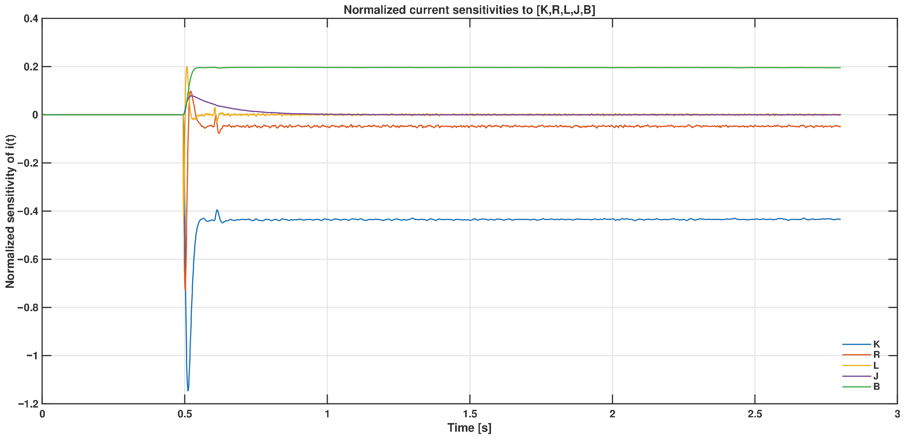
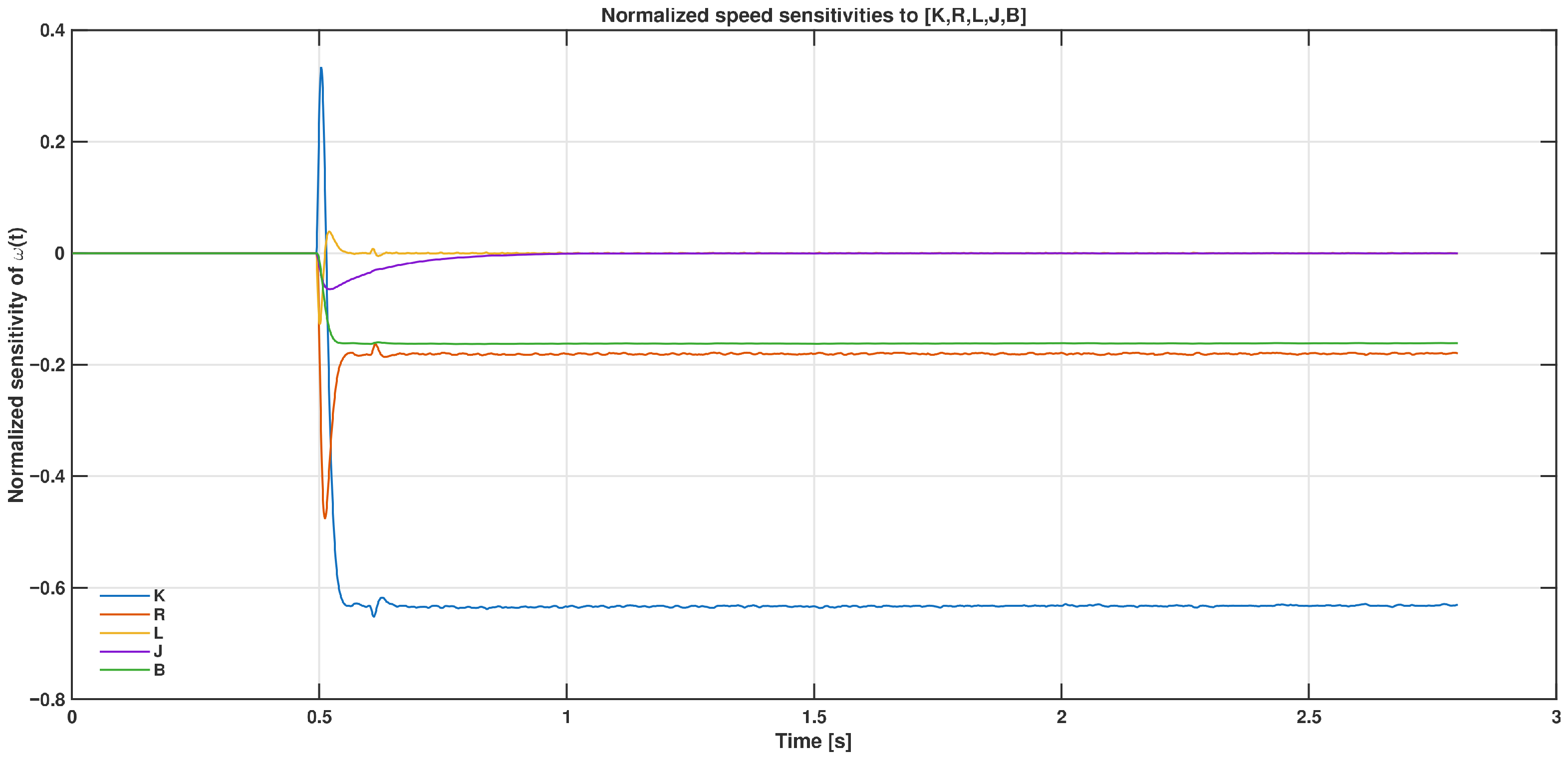
Figure 1 displays the normalized current sensitivities for the Mavilor motor, while Figure 2 shows the corresponding normalized speed sensitivities. Each parameter exhibits a clearly distinguishable temporal signature: K dominates the fast electromechanical interaction and produces the characteristic current dip; R and L primarily affect the sharp electrical transient; J shapes the medium–scale acceleration phase; and B influences the late decay and steady-state level of the speed. These distinct patterns indicate that the measured outputs respond differently to each parameter, suggesting good theoretical separability.

To formalize the separability of these signatures, the normalized sensitivities of current and speed were stacked into the matrix

$$S_{\mathrm{stack}}=\left[\begin{array}{c}{S}_i^{\mathrm{n}}\\ S_{\omega }^{\mathrm{n}}\end{array}\right]\in {\mathbb{R}}^{2N\times 5},$$

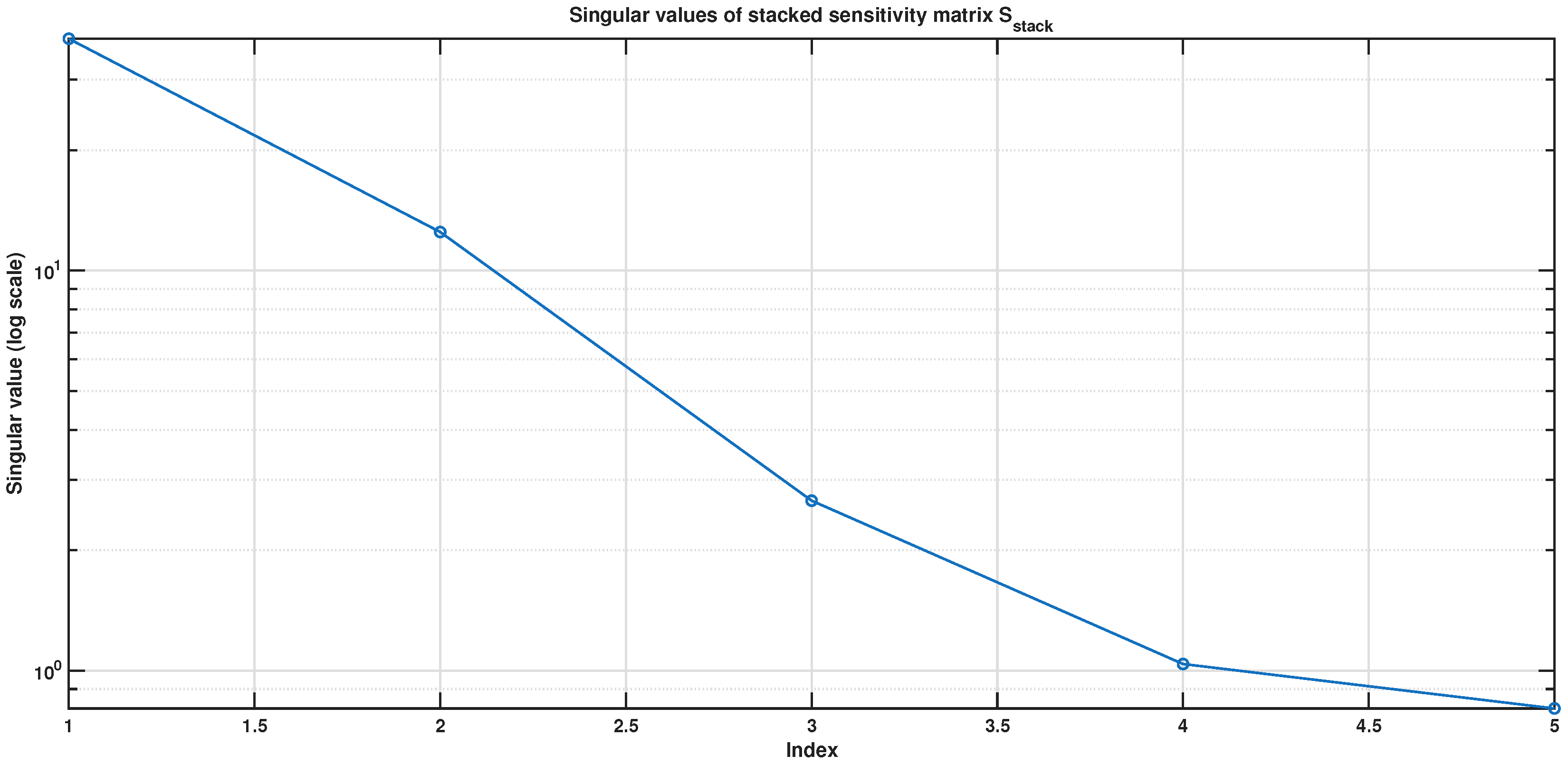
where N denotes the number of time samples. A singular–value decomposition of $S_{\mathrm{stack}}$ for the Mavilor experiment produced the strictly positive singular values

$${\sigma }_{\mathrm{CML}-050}=[37.98,12.49,2.66,1.04,0.80],$$

yielding $\mathrm{rank}\left(S_{\mathrm{stack}}\right)=5$ and a moderate condition number $\kappa \left(S_{\mathrm{stack}}\right)=47.2$. The full-column-rank property and the singular-value spectrum, summarized in Figure 3, confirm that all five parameters are structurally identifiable under the considered step–response excitation. Although L and J exhibit the smallest sensitivity magnitudes—a natural consequence of electrical–mechanical time-scale separation and encoder quantization—their signatures remain linearly independent. The practical implications of their weaker excitation are further examined through Monte Carlo analyses over randomized initializations in Section 4.5.

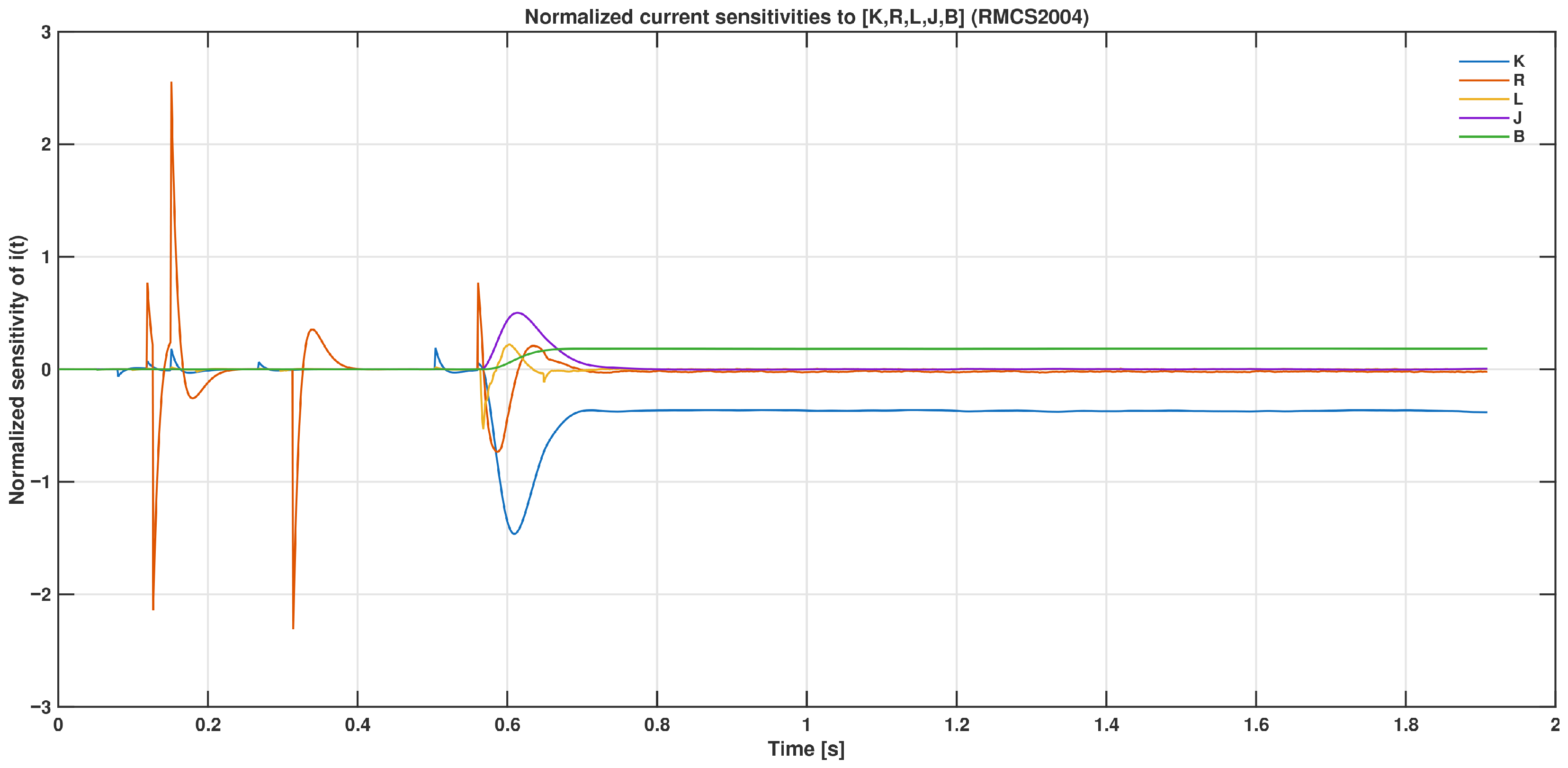
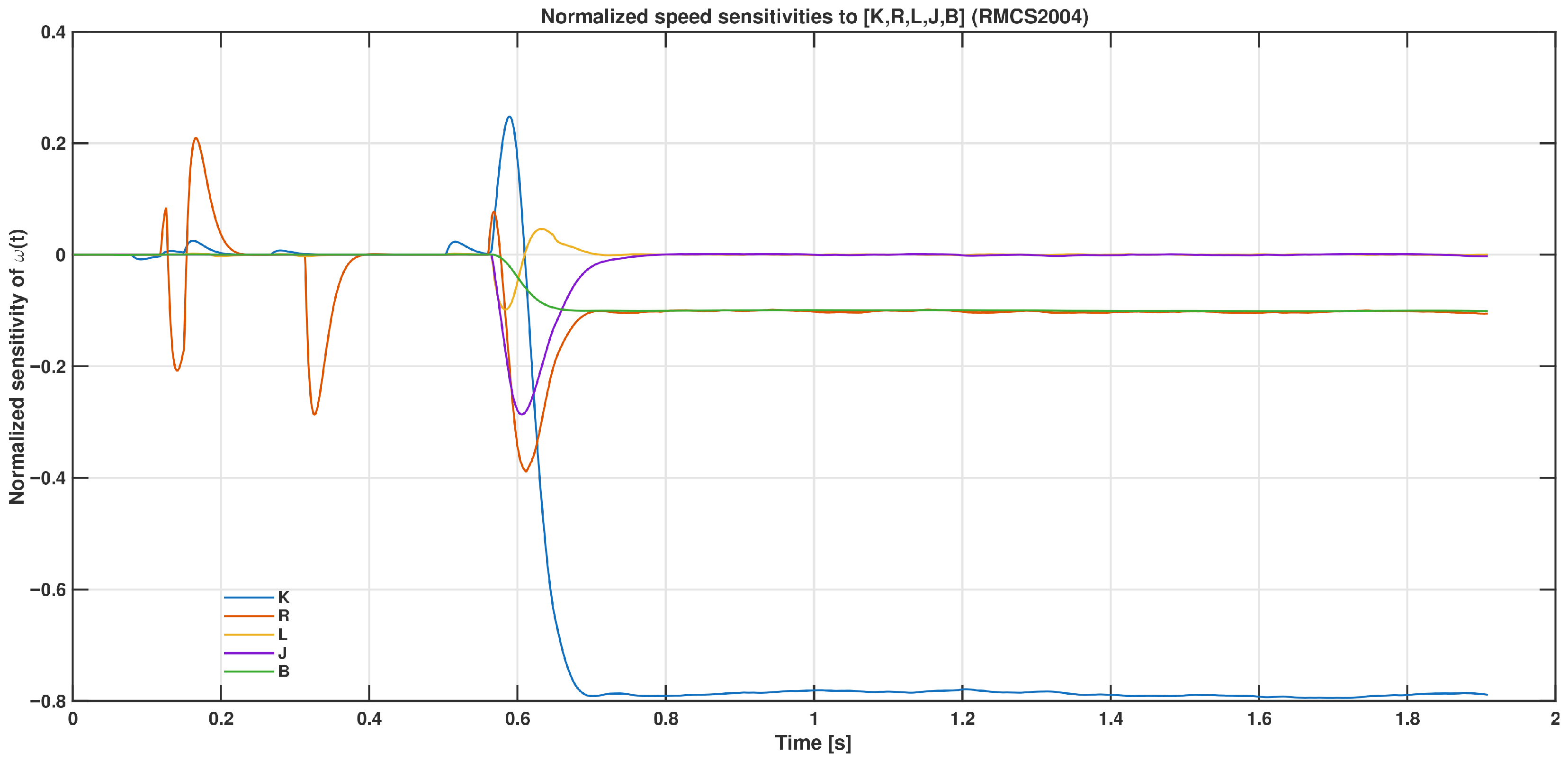
The same procedure was repeated for the RMCS2004 motor using the parameters identified from its real step response. The normalized current and speed sensitivities are shown in Figure 4 and Figure 5, respectively. As in the CML-050 case, each parameter exhibits a distinct temporal pattern: K and R dominate the sharp electrical transient, J and B shape the medium and long time scales of the speed response, and L mainly affects the current dynamics around the step onset. The relative magnitudes differ from those of the smaller motor, reflecting the higher inertia and lower resistance of the RMCS2004, but the qualitative separation between parameters is preserved.

Stacking the normalized current and speed sensitivities into the corresponding matrix $S_{\mathrm{stack}}\in {\mathbb{R}}^{2N\times 5}$ and performing an SVD yields the singular values

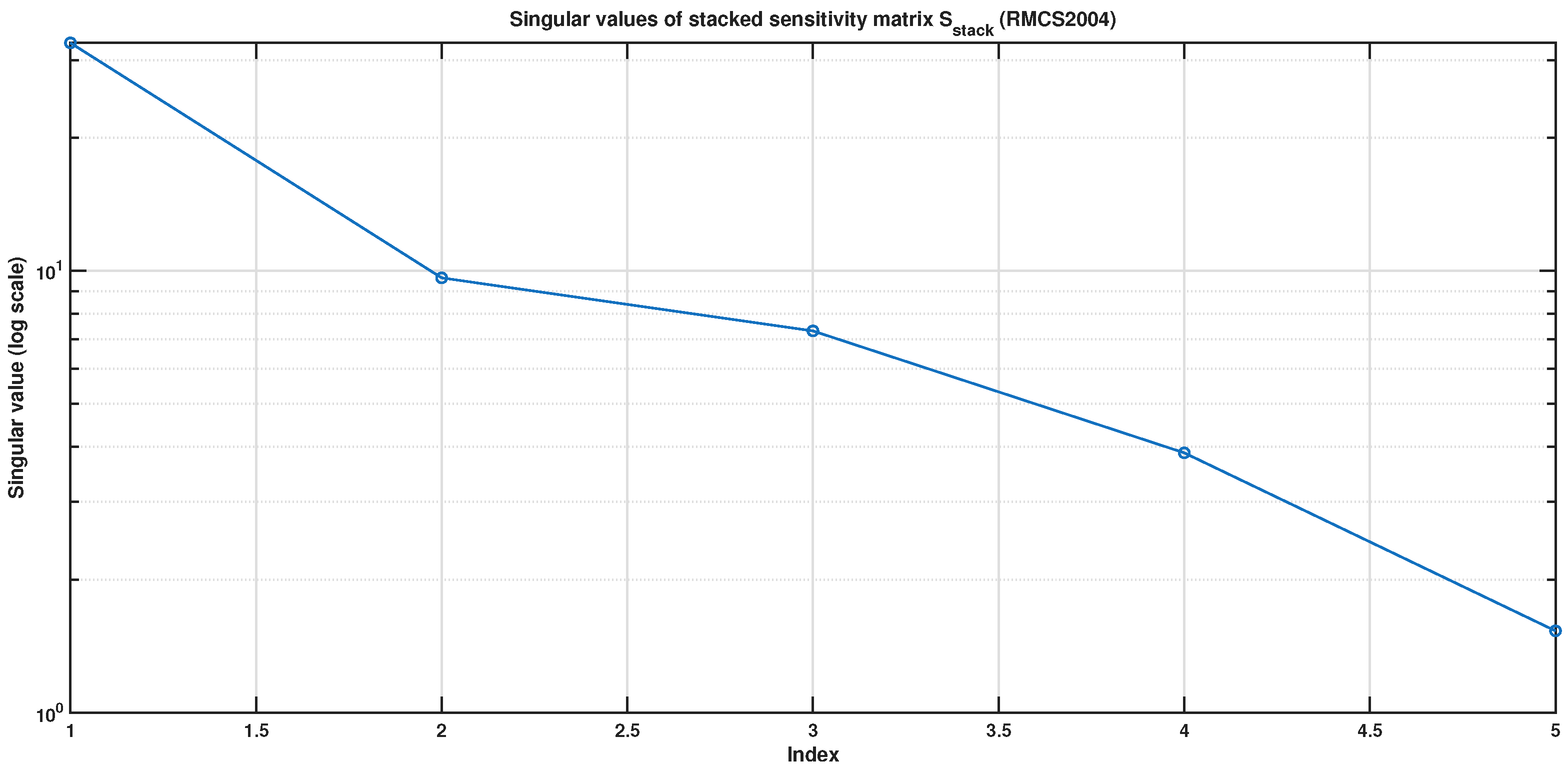
$${\sigma }_{\mathrm{RMCS}2004}=[32.81,9.64,7.32,3.88,1.53],$$

again with full column rank $\mathrm{rank}\left(S_{\mathrm{stack}}\right)=5$ and a condition number $\kappa \left(S_{\mathrm{stack}}\right)=21.4$ as shown in Figure 6. The tighter spread of singular values relative to the Mavilor case indicates slightly better conditioning of the parameter estimation problem for this actuator, despite its larger inertia and longer mechanical time constant.

These analyses confirm that the five-parameter model is structurally identifiable under the tested conditions. This supports the use of the proposed grey-box framework as a general tool for DC motor actuators.

4.2. Mavilor CML-050

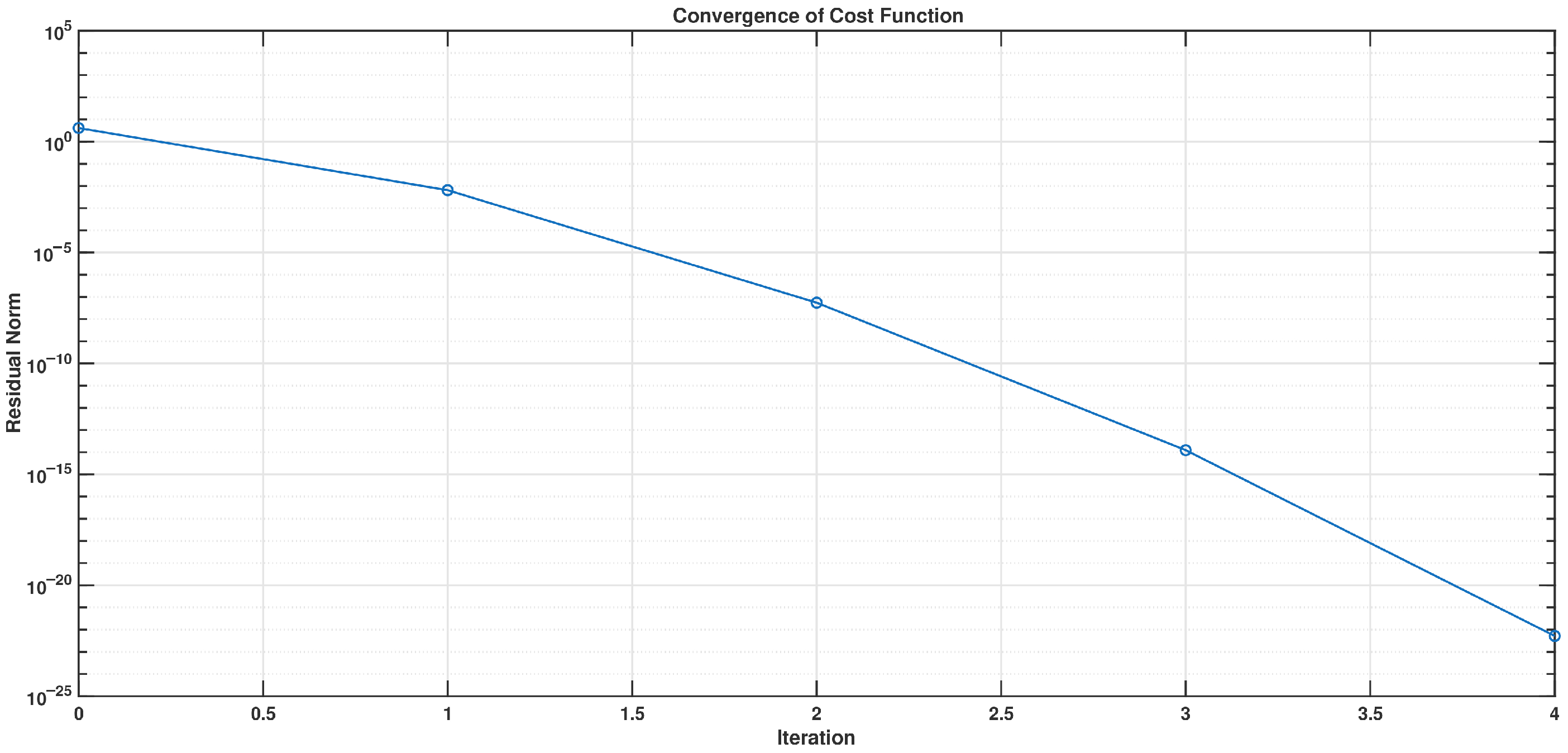
For the Mavilor motor, the nominal parameters used as initialization were $[0.048774,3.13631,0.01307,9.0\times {10}^{-6},1.69\times {10}^{-4}]$. Simulated tests with step inputs of 6 V and 8 V reduced the residual norm from $7.95$ to $4.2\times {10}^{-21}$ within five iterations, recovering the nominal parameters exactly. The estimated electrical and mechanical time constants were $t_e=4.17\mathrm{ms}$ and $t_m=11.9\mathrm{ms}$, yielding a damping ratio $\zeta =0.84$. Simulated and fitted trajectories overlapped almost perfectly, with ${\mathrm{NRMSE}}_{\omega },{\mathrm{NRMSE}}_i<{10}^{-3}\%$; the corresponding step responses and convergence behavior are illustrated in Figure 7 and Figure 8, respectively. These results confirm that the optimization process reconstructs the nominal dynamics accurately and that the normalization strategy balances the electrical and mechanical components effectively.

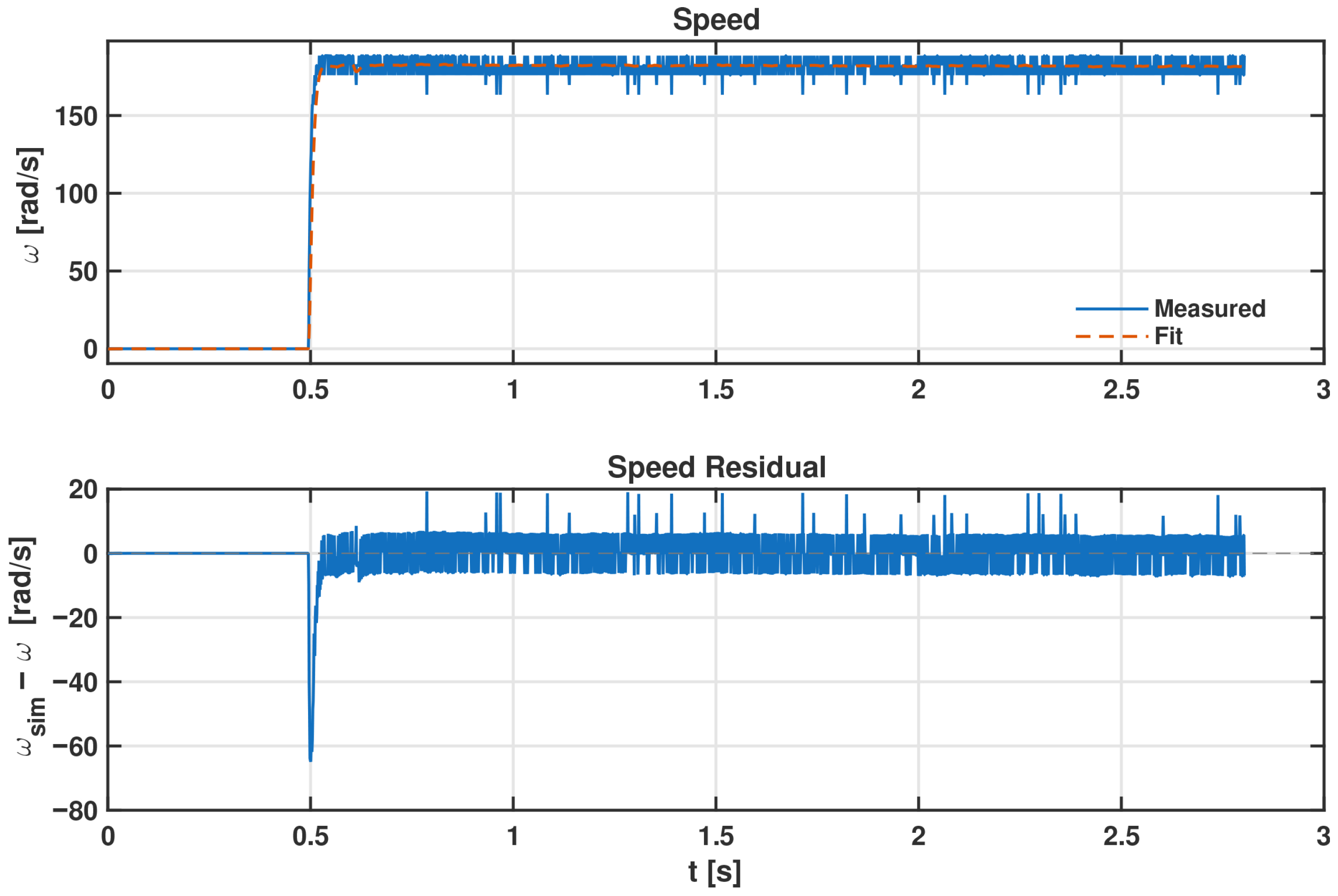
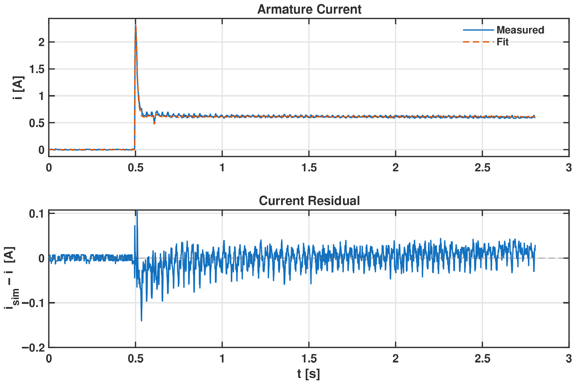
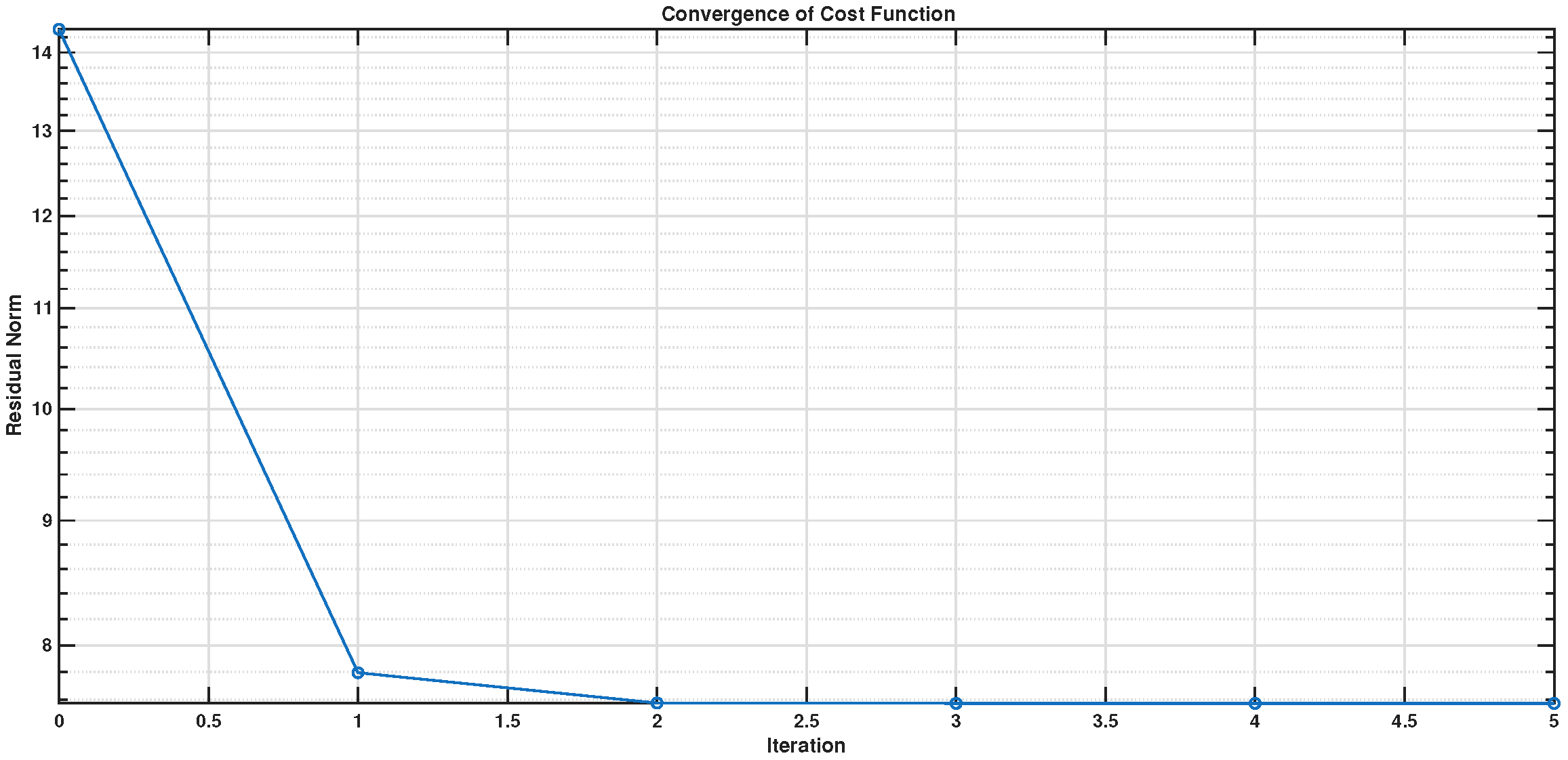
When applied to the unprocessed signals, the optimization converged after five iterations, reducing the residual norm from $14.31$ to $7.57$. The identified model reproduced the steady-state speed and current (see Figure 9 and Figure 10) with low normalized errors (${\mathrm{NRMSE}}_{\omega }=3.2\%$, ${\mathrm{NRMSE}}_i=0.92\%$). The corresponding time constants were $t_e=2.66\mathrm{ms}$ and $t_m=11.5\mathrm{ms}$, with a damping ratio $\zeta =1.04$.

The residual-norm evolution for this experiment is shown in Figure 11, where the cost decreases from $14.31$ to $7.57$ within five iterations. These results show that the estimator remains robust under encoder quantization and PWM ripple. The current-limit constraint was satisfied in all cases ($\mathrm{viol}=0$), confirming the effectiveness of the algebraic penalty.

Overall, the CML-050 results show that the proposed estimator preserves both convergence speed and physical interpretability, even when applied to raw, noisy signals. The low residuals and accurate steady-state reproduction indicate that the embedded algebraic constraints guide the optimizer toward physically admissible solutions without the need for filtering or parameter regularization.

4.3. Motor RMCS2004

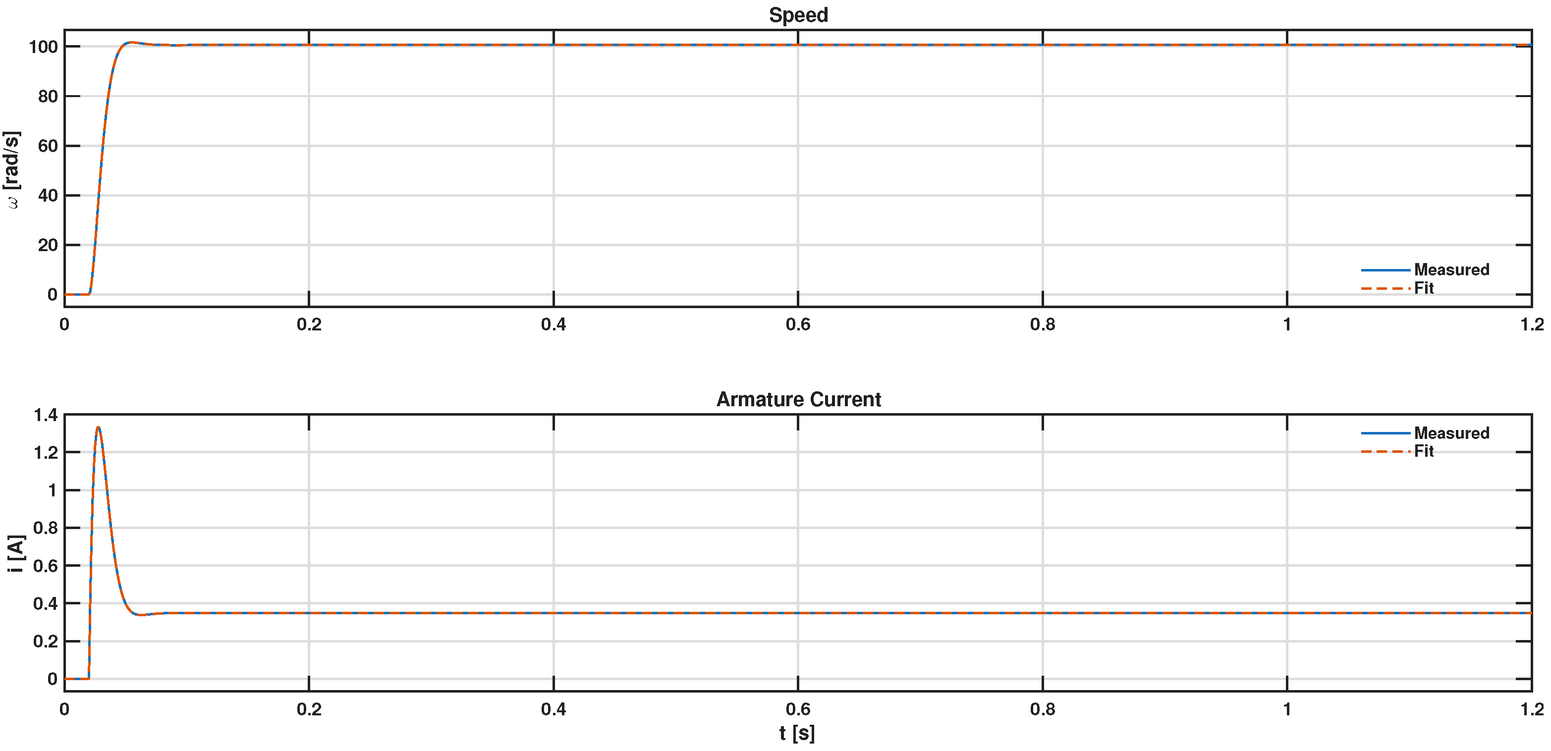
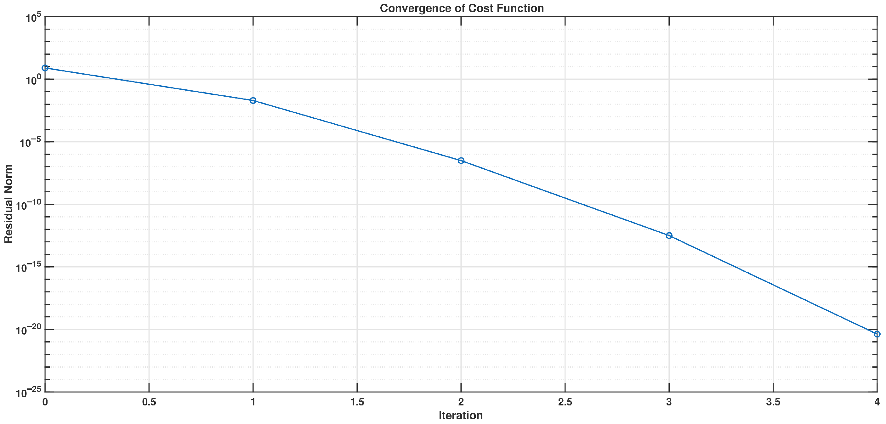
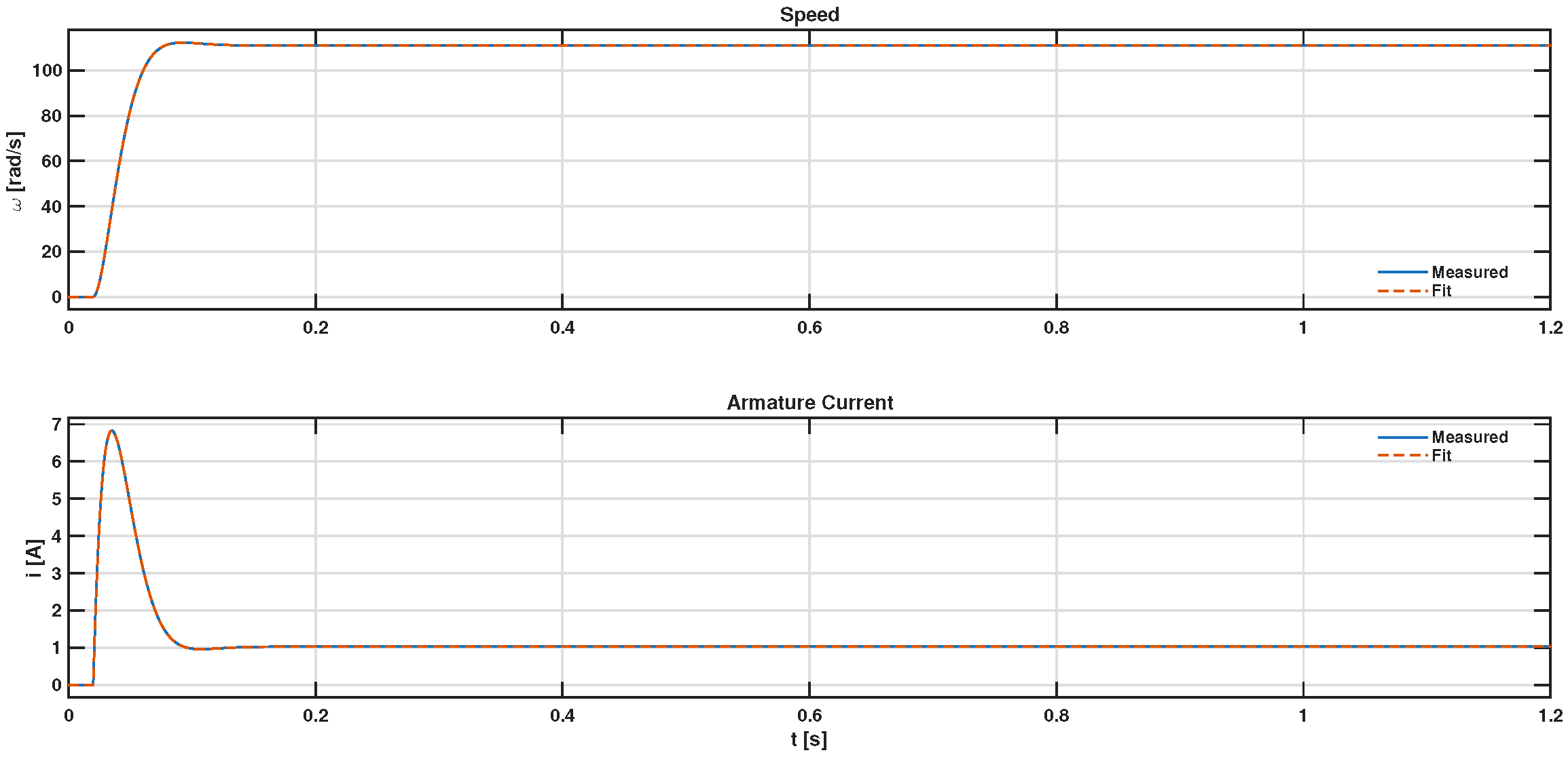
For the RMCS2004 motor, the nominal parameters from manufacturer data were $[0.073472,0.921042,0.007759,1.36\times {10}^{-4},6.78\times {10}^{-4}]$. A simulated 9.1 V step input reduced the residual norm from $4.11$ to $5.17\times {10}^{-23}$ within five iterations, indicating exact recovery of the nominal dynamics. The resulting time constants were $t_e=8.42\mathrm{ms}$ and $t_m=23.2\mathrm{ms}$, with $\zeta =0.83$. These ideal-condition results, illustrated in Figure 12 and Figure 13, illustrate the strong conditioning of the Levenberg–Marquardt search when the initialization lies within a physically admissible region.

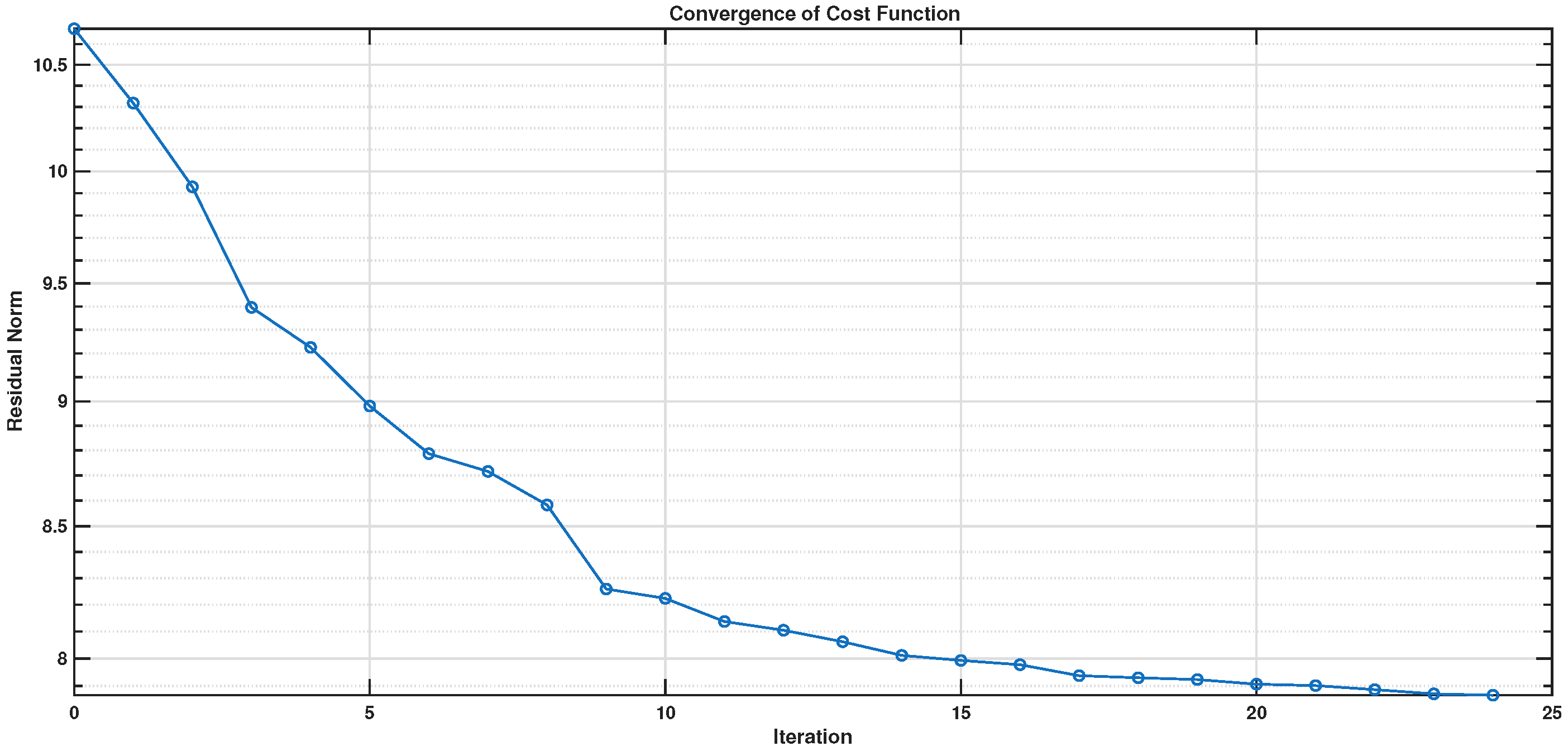
When tested on the real unfiltered dataset, the residual norm decreased from $10.68$ to $7.87$ after 25 iterations. The estimated parameters were as follows:

$$[K,R,L,J,B]=[0.07445,0.91030,6.46\times {10}^{-3},1.40\times {10}^{-4},6.96\times {10}^{-4}],$$

corresponding to electrical and mechanical time constants $t_e=7.10\mathrm{ms}$ and $t_m=23.0\mathrm{ms}$, and a damping ratio $\zeta =0.899$. The predicted steady-state values matched the measurements to within $1\%$ (${\omega }_{\mathrm{ss}}=111$ vs. $111\mathrm{rad}/\mathrm{s}$, $i_{\mathrm{ss}}=1.04$ vs. $1.05\mathrm{A}$), and the trajectory errors remained small (${\mathrm{NRMSE}}_{\omega }=2.63\%$, ${\mathrm{NRMSE}}_i=1.21\%$). The slightly underdamped transient is consistent with this actuator’s larger inertia and reduced viscous friction compared to the Mavilor unit.

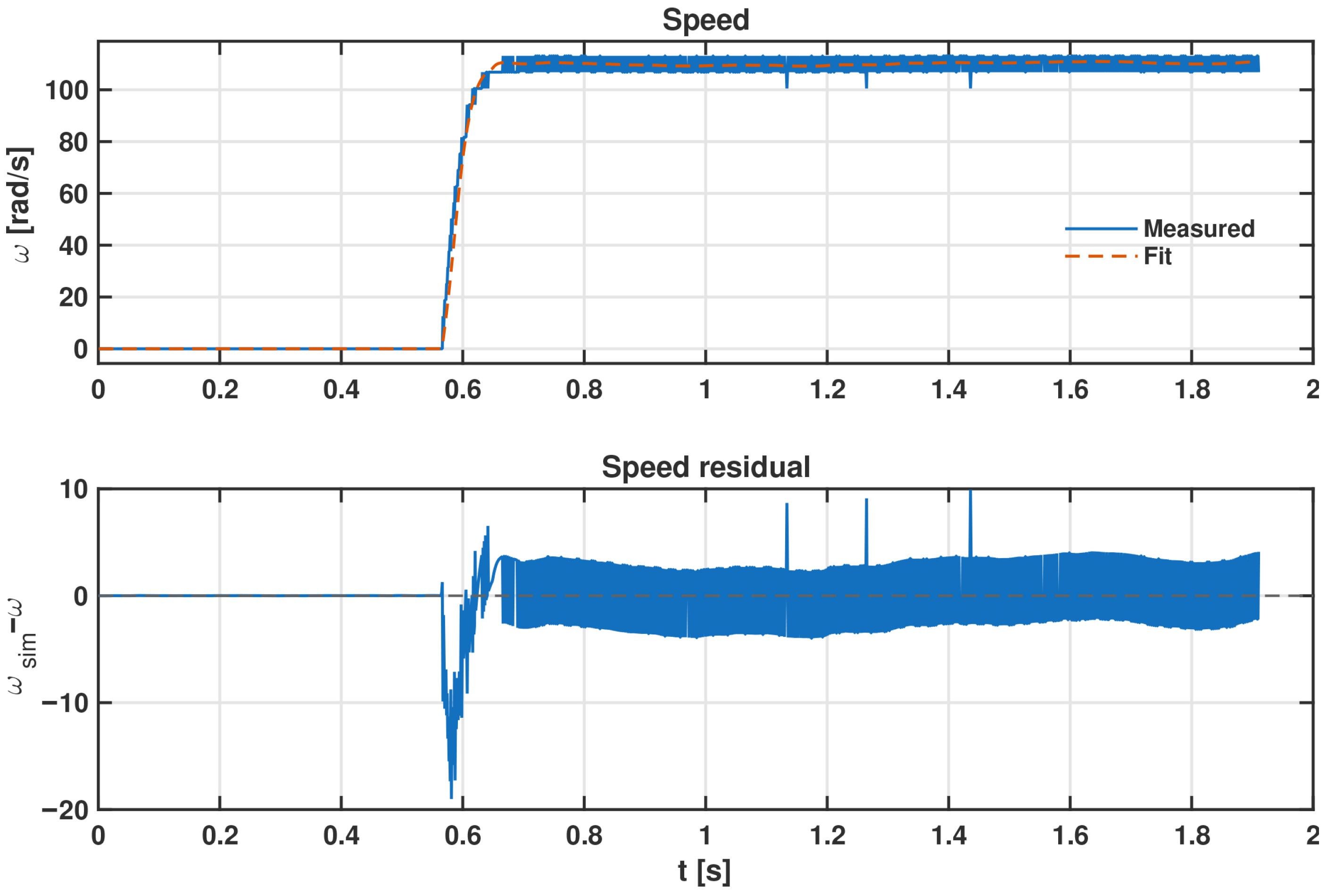
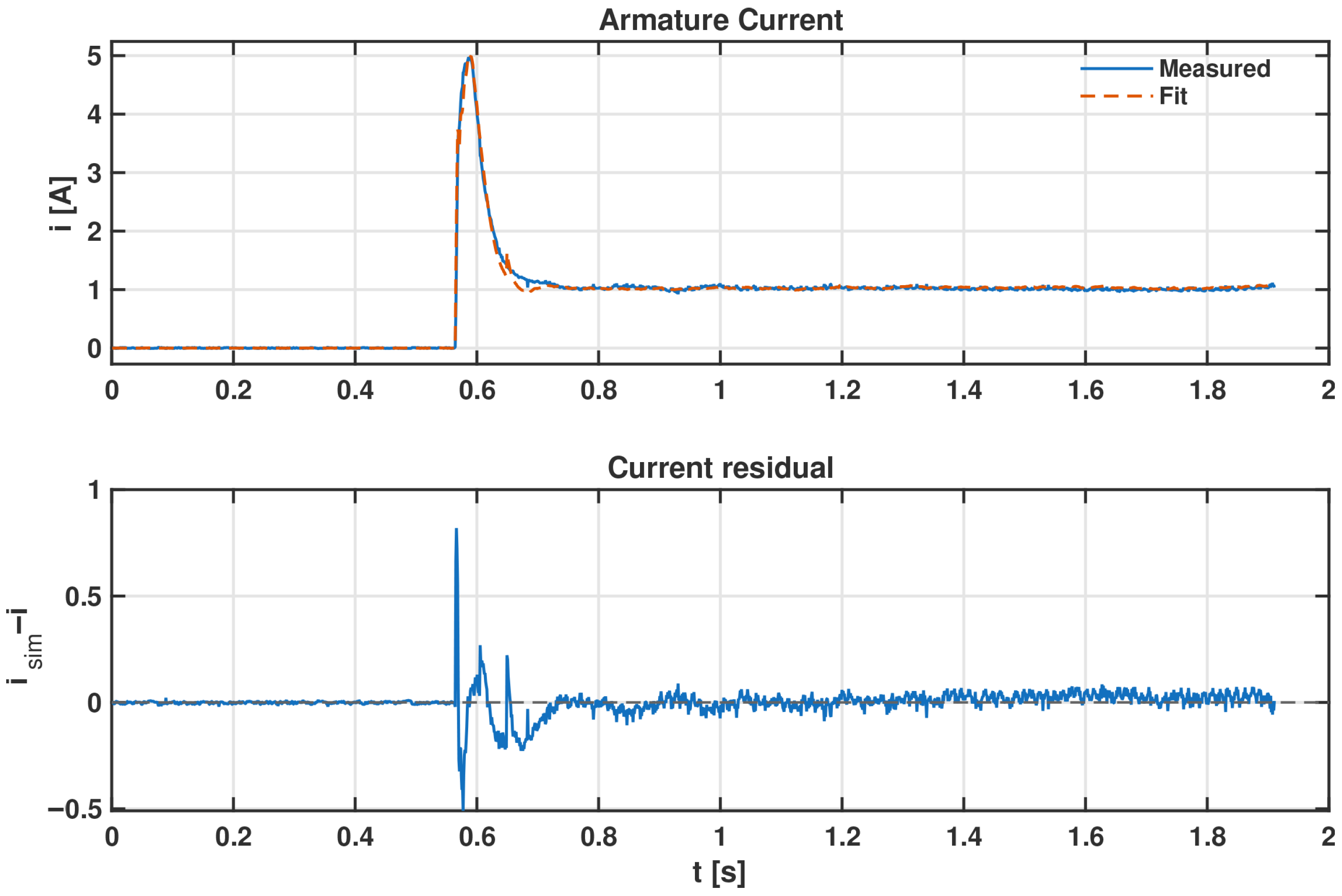
The measured and identified speed response is shown in Figure 14, while Figure 15 presents the corresponding current fit together with its residuals. The convergence behavior in Figure 16 exhibits a smooth monotonic decay, confirming stable numerical performance of the logarithmic reparameterization even under unfiltered encoder data.

Overall, the RMCS2004 identification results corroborate the findings obtained with the CML-050 motor: the proposed grey-box approach remains stable and physically meaningful even when applied to raw, unfiltered data. The strong agreement between simulated and experimental steady-state values highlights the consistency of the steady-state algebraic enforcement, while the low NRMSE values demonstrate accurate transient reproduction without digital smoothing.

4.4. Parameter Uncertainty: Gauss–Newton and Bootstrap Analysis

To complement the trajectory-based validation presented in the previous subsections, we quantified the uncertainty associated with each identified parameter using two complementary approaches: first, the local Gauss–Newton covariance approximation, based on the sensitivity Jacobian of the composite residual, and second, a nonparametric bootstrap dispersion analysis constructed from resampled trajectory residuals. This dual analysis provides both a local linear estimate of parameter sensitivity and an empirical measure of variability under measurement noise.

For each motor, the Jacobian matrix $J\left(\theta \right)$ was computed numerically around the final estimate ${\theta }_{\mathrm{ref}}$, and an approximate covariance matrix was obtained as

$$\mathrm{Cov}\left(\theta \right)\approx {\sigma }^2{\left(J^{\top }J\right)}^{-1},$$

where ${\sigma }^2$ denotes the normalized residual variance.

Table 2. Gauss–Newton standard deviations for both motors.

Motor	std$\left(\mathit{K}\right)$	std$\left(\mathit{R}\right)$	std$\left(\mathit{L}\right)$	std$\left(\mathit{J}\right)$	std$\left(\mathit{B}\right)$
Mavilor CML-050	$4.80\times {10}^{-5}$	$1.37\times {10}^{-2}$	$7.14\times {10}^{-5}$	$4.62\times {10}^{-8}$	$2.01\times {10}^{-7}$
RMCS2004	$4.10\times {10}^{-5}$	$2.80\times {10}^{-3}$	$4.39\times {10}^{-5}$	$4.10\times {10}^{-7}$	$1.09\times {10}^{-6}$

summarizes the resulting standard deviations. Both actuators exhibit extremely small dispersions for all parameters, confirming the strong conditioning reported in the structural identifiability study (Section 4.1).

A bootstrap analysis with $B=200$ resamples was performed by re-generating synthetic measurement trajectories from the fitted model plus resampled residuals, recomputing the local Jacobian for each trial, and drawing Gaussian perturbations using the corresponding covariance. The empirical 2.5–97.5 percentiles of the resulting distribution yield a 95% confidence interval for each parameter. The intervals listed in

Table 3. Bootstrap 95% confidence intervals for both motors (rounded).

Motor	$\mathit{K}$	$\mathit{R}$	$\mathit{L}$	$\mathit{J}$	$\mathit{B}$
Mavilor	$[0.05,0.05]$	$[3.09,3.15]$	$[8.18\times {10}^{-3},8.47\times {10}^{-3}]$	$[8.24\times {10}^{-6},8.41\times {10}^{-6}]$	$[1.60\times {10}^{-4},1.60\times {10}^{-4}]$
RMCS2004	$[0.07,0.07]$	$[0.91,0.92]$	$[6.37\times {10}^{-3},6.53\times {10}^{-3}]$	$[1.39\times {10}^{-4},1.41\times {10}^{-4}]$	$[6.94\times {10}^{-4},6.98\times {10}^{-4}]$

are narrow and fully consistent with the Gauss–Newton dispersions, providing strong evidence of robustness under raw, unfiltered signals.

Across both actuators, the uncertainty magnitudes remain small relative to the nominal parameter scales, and the confidence intervals do not overlap substantially between K, R, L, J, and B, reinforcing the practical separability predicted by the sensitivity and SVD analysis in Section 4.1. Moreover, the agreement between Gauss–Newton and bootstrap metrics indicates that the residual normalization and embedded physical constraints yield a well-behaved optimization landscape, even under encoder quantization and PWM ripple. The narrow dispersion in J and B, despite low-frequency noise in the speed signal, further demonstrates the effectiveness of combining transient information with steady-state algebraic penalties. Additional experiments in which ${\lambda }_{\mathrm{ss}}$ and ${\lambda }_{\mathrm{pk}}$ were varied within one order of magnitude yielded negligible changes in the identified parameters, which is consistent with the normalization strategy and the log-parameter formulation used in the optimization.

4.5. Robustness to Initial Conditions

Beyond structural identifiability, it is crucial to evaluate the sensitivity of the proposed grey-box estimator to poor or highly distorted initial guesses of the parameter vector. To this end, we conducted Monte Carlo experiments in which the Levenberg–Marquardt solver was repeatedly initialized from randomized perturbations of the reference solution, while keeping all other settings (log-parameterization, residual normalization, ODE tolerances, and constraints) identical to those used in the main identification runs.

Given a reference parameter vector ${\mathit{\theta }}_{\mathrm{ref}}$ obtained from the experimental step response of each motor, we generated randomized initial guesses of the form

$${\mathit{\theta }}_0={\mathit{\theta }}_{\mathrm{ref}}\odot \rho ,{\rho }_j\sim {\mathcal{U}}_{log}(0.25,4.0),$$

(6)

where ${\mathcal{U}}_{log}$ denotes a log-uniform distribution over $[0.25,4.0]$, and ⊙ is the element-wise product. In other words, each parameter was independently scaled between $25\%$ and $400\%$ of its reference value before optimization. For each run, the solver operated in log-parameter space, $\mathit{\theta }=\mathbf{s}\odot e^{\mathbf{z}}$, thereby enforcing strict positivity and improving numerical conditioning.

To quantify robustness, two metrics were monitored:

$$\mathrm{rel}.\mathrm{err}={\displaystyle \frac{\parallel \widehat{\mathit{\theta }}-{\mathit{\theta }}_{\mathrm{ref}}{\parallel }_2}{\parallel {\mathit{\theta }}_{\mathrm{ref}}{\parallel }_2}},{\mathrm{NRMSE}}_{\omega }={\displaystyle \frac{\sqrt{\frac{1}{N}{\sum }_{k=1}^N{\left({\omega }_{\mathrm{sim}}(t_k;\widehat{\mathit{\theta }})-\omega \left(t_k\right)\right)}^2}}{{max}_k\omega \left(t_k\right)-{min}_k\omega \left(t_k\right)}}.$$

(7)

A run was classified as a “good fit” if it satisfied $\mathrm{rel}.\mathrm{err}\le 0.5$ and ${\mathrm{NRMSE}}_{\omega }\le 0.10$ (10%), which are conservative thresholds compared with the errors achieved in the main identification experiments.

For the Mavilor CML-050 motor, 100 randomized initializations were tested. In all cases, the algorithm terminated with finite residual norm and physically admissible parameters ($\mathit{\theta }>0$), without numerical failure or violation of the current-limit constraint. The vast majority of runs converged back to the same basin of attraction as the reference solution, with ${\mathrm{NRMSE}}_{\omega }$ remaining close to the nominal value reported in Section 4 and only a few runs exhibiting slightly larger but still acceptable trajectory errors. Even when individual parameters were simultaneously mis-scaled by factors approaching $4\times$ their reference values, the fitted models continued to reproduce the measured step responses with small deviations in speed and current.

A more extensive experiment was performed for the RMCS2004 actuator, using $N_{\mathrm{runs}}=100$ randomized initializations within the same $[0.25,4.0]$ range. According to the criteria in (7), 89 runs were classified as good fits, while 11 runs exhibited larger parameter deviations and were therefore classified as poor fits. Among the good fits, the statistics were as follows:

$$\mathrm{rel}.\mathrm{err}=0.214\pm 0.042,\mathrm{rel}.{\mathrm{err}}_{min}=0.055,\mathrm{rel}.{\mathrm{err}}_{max}=0.377,$$

$${\mathrm{NRMSE}}_{\omega }=(2.73\pm 0.02)\%,{\mathrm{NRMSE}}_{\omega ,min}=2.69\%,{\mathrm{NRMSE}}_{\omega ,max}=2.83\%.$$

For the group of poor-fit runs, the average trajectory error remained moderate, with ${\mathrm{NRMSE}}_{\omega }\approx 4.94\%$, and no run produced nonphysical (negative) parameters. In practice, most good-fit runs converged to nearly indistinguishable parameter vectors and error levels, indicating a large basin of attraction around the physically plausible solution.

These Monte Carlo experiments over random initializations show that the proposed constrained grey-box formulation is only weakly sensitive to the choice of initial parameters. The combination of log-parameterization, steady-state algebraic penalties, and the current-limit constraint effectively guides the optimizer toward a robust basin of attraction in parameter space, even when starting from initial guesses that deviate by more than one order of magnitude from the final estimates. This empirical robustness complements the structural identifiability analysis of Section 4.1 and addresses practical concerns about convergence from poor starting points.

4.6. Comparison Against a Standard Least-Squares Baseline

To contextualize the performance of the proposed constrained grey-box estimator, we include a comparison against the most widely used baseline method in classical DC motor identification: the ordinary least-squares (LS) approach. LS is the standard entry-level technique in laboratory system identification because it is simple, algebraically direct, and does not require nonlinear optimization or embedded physical constraints. For these reasons, LS constitutes an appropriate baseline to evaluate the added value of enforcing physics-based consistency.

However, LS is also known to suffer from several limitations: it cannot guarantee positivity of $\{L,J,B,R\}$, it is highly sensitive to noise and voltage delays, and it does not incorporate steady-state algebraic consistency. These issues commonly produce nonphysical estimates or poor transient matching when applied to unfiltered laboratory data. The comparison against LS, therefore, highlights the contribution of the proposed constrained formulation.

Table 4. Comparison between the proposed constrained grey-box identification method and a standard least-squares baseline for both actuators. The proposed method yields lower errors and physically coherent parameters, whereas LS exhibits higher NRMSE and, in the case of the Mavilor motor, a nonphysical inductance.

Motor	Method	${\mathbf{NRMSE}}_{\mathit{\omega }}$ [%]	${\mathbf{NRMSE}}_{\mathit{i}}$ [%]	SS err $\mathit{\omega }$ [%]	SS err i [%]	Notes
Mavilor	Proposed	3.20	0.92	0.35	3.40	Physically consistent
	LS baseline	5.12	7.99	0.35	3.40	$L<0$ (corrected to $\left|L\right|$ for simulation)
RMCS	Proposed	2.63	1.21	1.38	8.86	Physically consistent
	LS baseline	19.61	11.09	1.38	8.86	Large transient mismatch

summarizes the metrics obtained for both actuators when using LS and the proposed method under identical experimental conditions.

Overall, LS struggles to accurately reconstruct the transient dynamics accurately, particularly for the RMCS2004 actuator, where ${\mathrm{NRMSE}}_{\omega }$ approaches $20\%$. For the Mavilor motor, LS even produces a negative inductance, confirming the sensitivity of the method to noise and voltage-delay artifacts. In contrast, the proposed method consistently achieves low NRMSE, enforces physical consistency, and remains robust without requiring signal filtering. These results underscore the benefits of embedding electromechanical constraints and steady-state algebra into the identification process.

4.7. Comparative Analysis

Table 5. Summary of identification results for both motors; low NRMSE, near-unity damping, and consistent time constants reflect robust and physically coherent fits across scales.

Motor	Dataset	${\mathbf{NRMSE}}_{\mathit{\omega }}$ [%]	${\mathbf{NRMSE}}_{\mathit{i}}$ [%]	${\mathit{t}}_{\mathit{e}}$ [ms]	${\mathit{t}}_{\mathit{m}}$ [ms]	$\mathit{\zeta }$
Mavilor CML-050	Simulated	0.00	0.00	4.17	11.9	0.84
Mavilor CML-050	Real (unfiltered)	3.20	0.92	2.66	11.5	1.04
RMCS2004	Simulated	0.00	0.00	8.42	23.2	0.83
RMCS2004	Real (unfiltered)	2.63	1.21	7.10	23.0	0.90

summarizes the main metrics obtained in simulation and experiment for both motors. In all cases, the optimizer converged smoothly from nominal seeds and produced parameter sets that remained physically interpretable. The damping ratios stayed close to unity, indicating well-damped electromechanical behavior, while the steady-state penalties ensured algebraic consistency without manual tuning. Convergence typically required 5–25 iterations, depending on noise and initialization, demonstrating stability across different scales and operating voltages.

Additionally,

Table 6. Identified parameters on real (unfiltered) data; estimated values are physically plausible and aligned with datasheet scales.

Motor	K	R	L	J	B	${\mathit{t}}_{\mathit{e}}$ [ms]	${\mathit{t}}_{\mathit{m}}$ [ms]	$\mathit{\zeta }$	NRMSEω/NRMSEi
Mavilor	0.04744	3.1208	$8.32\times {10}^{-3}$	$8.32\times {10}^{-6}$	$1.60\times {10}^{-4}$	2.66	11.5	1.04	3.20/0.92 (%)
RMCS2004	0.07445	0.91030	$6.46\times {10}^{-3}$	$1.40\times {10}^{-4}$	$6.96\times {10}^{-4}$	7.10	23.0	0.899	2.63/1.21 (%)

lists the identified physical parameters for both real cases, evidencing the coherence and plausibility of all estimates relative to manufacturer data. The observed differences between the two actuators align with their design characteristics: the RMCS2004, with larger inertia and lower resistance, exhibits slower transients and slightly lower damping than the smaller Mavilor unit. This trend confirms that the proposed estimator correctly adapts to different dynamic scales while maintaining convergence behavior and physical admissibility.

Across both actuators, the proposed framework identified coherent and physically plausible parameters with minimal residuals and negligible constraint violations. The combined enforcement of steady-state algebra and current limits prevented unrealistic overshoots or parameter drift, even under noisy conditions. These results demonstrate that the method achieves robustness, physical interpretability, and cross-motor generality without requiring filtering or extensive preprocessing. The close agreement between predicted and measured steady-state values further supports the benefit of embedding steady-state algebra directly into the cost function.

Although the experimental validation focused on two permanent-magnet DC motors, these actuators differ substantially in electrical resistance, inertia, and torque constant, providing an initial indication that the proposed formulation scales across distinct electromechanical regimes. Broader validation on additional motor families would be necessary to establish full generality, especially for coreless or very high-speed units where iron losses and torque ripple become more relevant, or for geared actuators with substantial friction and backlash. These cases may require more detailed friction or loss models and richer excitation signals.

Regarding measurement quality, the method was intentionally applied to raw, unfiltered data so that encoder quantization, PWM ripple, and current-sensor noise appear directly in the residual. These effects are not modeled explicitly; instead, they are treated as bounded disturbances mitigated by RMS normalization and by the physical constraints embedded in the cost, which prevent noise-driven parameter drift. More explicit modeling of measurement imperfections, such as quantization-aware residuals or probabilistic noise representations, could enhance robustness and refine uncertainty estimates, although this lies outside the present scope.

5. Conclusions

This study presents a unified grey-box identification framework for permanent-magnet DC motors that integrates electromechanical coupling, steady-state algebraic consistency, and physical constraints directly into the optimization process. The method minimizes a normalized residual that combines current and velocity trajectories with algebraic and current-limit penalties, ensuring physically meaningful steady-state behavior and well-bounded transients without requiring digital filtering or manual parameter tuning.

The formulation was validated on two actuators of different electrical and mechanical scales—Mavilor CML-050 and RMCS2004—under simulated and unfiltered measured conditions. Across all tests, the algorithm achieved sub-percent steady-state mismatches, low normalized trajectory errors (below 3%), and physically admissible parameter ratios. These results demonstrate robustness to quantization effects, PWM ripple, and sensor noise. The stable convergence and coherent parameter estimates for two distinct motor types highlight the generality of the proposed approach and its applicability to laboratory and robotic settings where model fidelity and experimental simplicity are critical.

Future work will extend the framework to multi-input electromechanical systems and dynamic friction models, and incorporate stochastic noise representations and Bayesian uncertainty quantification. These extensions will enable probabilistic assessments of parameter credibility and further strengthen the link between physics-based identification and data-driven adaptation in real robotic actuation environments.

References

1. Clochiatti, E.; Scalera, L.; Boscariol, P.; Gasparetto, A. Electro-mechanical Modeling and Identification of the UR5 e-series Robot. Robotica 2024, 42, 2430–2452. [Google Scholar] [CrossRef]
2. Gökçe, C.O.; İpek, M.E.; Dayıoğlu, M.; Ünal, R. Parameter estimation and speed control of real DC motor with low resolution encoder. Results Control Optim. 2025, 19, 100549. [Google Scholar] [CrossRef]
3. Fazdi, M.F.; Hsueh, P.W. Parameters Identification of a Permanent Magnet DC Motor: A Review. Electronics 2023, 12, 2559. [Google Scholar] [CrossRef]
4. Traversaro, S.; Del Prete, A.; Muradore, R.; Natale, L.; Nori, F. Inertial parameter identification including friction and motor dynamics. In Proceedings of the 2013 13th IEEE-RAS International Conference on Humanoid Robots (Humanoids), Atlanta, GA, USA, 15–17 October 2013; pp. 68–73. [Google Scholar] [CrossRef]
5. Wu, W. DC Motor Parameter Identification Using Speed Step Responses. Model. Simul. Eng. 2012, 2012, 189757. [Google Scholar] [CrossRef]
6. Hernández, J.; Cruz, A.; López, R. Identificación de parámetros dinámicos de motores de corriente directa usando el método de Steiglitz–McBride. Mecatrónica Méx. 2019, 8, 14–23. [Google Scholar]
7. Siddiqi, F.U.R.; Ahmad, S.; Akram, T.; Ali, M.U.; Zafar, A.; Lee, S.W. Artificial Neural Network-Based Data-Driven Parameter Estimation Approach: Applications in PMDC Motors. Mathematics 2024, 12, 3407. [Google Scholar] [CrossRef]
8. Kim, P.S.; Kim, S.M.; Kim, S.Y. Model Parameter Identification for DC Motor Using Rapid Control Prototyping System. In Proceedings of the 2024 International Conference on Artificial Intelligence in Information and Communication (ICAIIC), Osaka, Japan, 19–22 February 2024; pp. 816–819. [Google Scholar] [CrossRef]
9. Wee, H.S.H.; Ahmad, N.S. Review and Comparative Analysis of System Identification Methods for Perturbed Motorized Systems. Comput. Model. Eng. Sci. 2025, 143, 1301–1354. [Google Scholar] [CrossRef]
10. Jimenez-Gonzalez, J.; Gonzalez-Montañez, F.; Jimenez-Mondragon, V.M.; Liceaga-Castro, J.U.; Escarela-Perez, R.; Olivares-Galvan, J.C. Parameter Identification of BLDC Motor Using Electromechanical Tests and Recursive Least-Squares Algorithm: Experimental Validation. Actuators 2021, 10, 143. [Google Scholar] [CrossRef]
11. Chakraborty, A.; Saha, R.; Halder, R. System identification of servo drive using simulation-based parameter estimation. ISA Trans. 2021, 113, 130–142. [Google Scholar] [CrossRef]
12. Hadef, M.; Mekideche, M.R. Parameter Identification of a Separately Excited DC Motor via Inverse Problem Methodology. Turk. J. Electr. Eng. Comput. Sci. 2009, 17, 99–106. [Google Scholar] [CrossRef]
13. Hassan, M.M.; Aly, A.A.; Rashwan, A.F. Different identification methods with application to a DC motor. J. Eng. Appl. Sci. 2007, 56, 401–412. [Google Scholar] [CrossRef]
14. Hamza, B.; El Mehdi, A.S.A.; Houcine, C.; Mouloud, D. A New Method for the Parametric Identification of DC Machines Using MATLAB Identification Toolbox and Experimental Measurements. In Proceedings of the International Conference on Energy and Green Computing (ICEGC 2021), Meknes, Morocco, 9–10 December 2021; Volume 284, p. 00007. [Google Scholar] [CrossRef]
15. Munciño, D.M.; Damian-Ramírez, E.A.; Cruz-Fernández, M.; Montoya-Santiyanes, L.A.; Rodríguez-Reséndiz, J. Metaheuristic and Heuristic Algorithms-Based Identification Parameters of a Direct Current Motor. Algorithms 2024, 17, 209. [Google Scholar] [CrossRef]
16. Jesenik, M.; Ravber, M.; Trbušić, M. Innovative Approach for the Determination of a DC Motor’s and Drive’s Parameters Using Evolutionary Methods and Different Measured Current and Angular Speed Responses. Mathematics 2024, 12, 42. [Google Scholar] [CrossRef]
17. Demirtas, M.; Efe, M.O. Practical Parameter Identification of DC Motor Using Rapid Control Prototyping System. J. Electr. Eng. Technol. 2020, 15, 1101–1112. [Google Scholar]
18. Arévalo, E.; Herrera Hernández, R.; Katselis, D.; Reusser, C.; Carvajal, R. On Modelling and State Estimation of DC Motors. Actuators 2025, 14, 160. [Google Scholar] [CrossRef]
Figure 1. Normalized current sensitivities for the Mavilor CML-050 motor. The curves show the dimensionless influence of each parameter [ K , R , L , J , B ] on the armature current trajectory under a single voltage step. Each parameter exhibits a distinct temporal signature, indicating good separability at the electrical time scale.
Information 16 01079 g001
Figure 2. Normalized speed sensitivities for the Mavilor CML-050 motor. The parameters K, J, and B dominate the medium and long time scales, while R and L mainly affect the early transient. The distinct profiles across parameters support structural identifiability of the full set { K , R , L , J , B } from step–response data.
Information 16 01079 g002
Figure 3. Singular values of the stacked sensitivity matrix S stack for the Mavilor CML-050 identification. All five singular values are strictly positive, and the moderate spread ( κ ( S stack ) = 47.2 ) confirms full column rank and structural identifiability of the five parameters under the considered step experiment.
Information 16 01079 g003
Figure 4. Normalized current sensitivities for the RMCS2004 motor. Despite the different electrical and mechanical scales, each parameter retains a distinct influence on the armature current, supporting identifiability at the electrical time scale.
Information 16 01079 g004
Figure 5. Normalized speed sensitivities for the RMCS2004 motor. Parameters K, J, and B dominate the speed dynamics at medium and long time scales, while R and L mainly affect the early transient, mirroring the qualitative structure observed for the CML-050 actuator.
Information 16 01079 g005
Figure 6. Singular values of the stacked sensitivity matrix S stack for the RMCS2004 identification. All five values are strictly positive and the condition number ( κ ( S stack ) = 21.4 ) confirms good conditioning and full structural identifiability of { K , R , L , J , B } under the step experiment.
Information 16 01079 g006
Figure 7. Simulated step response and identified model for the Mavilor CML-050 motor; simulated and fitted trajectories are visually indistinguishable, confirming exact recovery of nominal parameters.
Information 16 01079 g007
Figure 8. Residual-norm convergence in the simulated identification (Mavilor CML-050); the cost decays by over twenty orders of magnitude within five iterations, evidencing rapid and well-conditioned optimization.
Information 16 01079 g008
Figure 9. Measured and identified speed response of the Mavilor CML-050. The top subplot shows the unfiltered measured speed and the identified model prediction. The bottom subplot presents the speed residual ( ω sim ω ), highlighting the low tracking error despite sensor noise and PWM ripple.
Information 16 01079 g009
Figure 10. Measured and identified armature current response of the Mavilor CML-050. The top subplot shows the unfiltered measured current and the identified model prediction. The bottom subplot presents the current residual ( i sim i ), illustrating the low modeling error even under quantization noise and PWM ripple.
Information 16 01079 g010
Figure 11. Residual-norm convergence on the experimental dataset (Mavilor CML-050); the smooth, monotonic decay indicates stable gradients and consistent numerical behavior on unfiltered data.
Information 16 01079 g011
Figure 12. Simulated step response and identified model for the RMCS2004 motor; the perfect overlap validates the solver configuration and residual normalization under ideal conditions.
Information 16 01079 g012
Figure 13. Residual-norm convergence in the simulated RMCS2004 identification; near-instant convergence confirms that the nominal parameters are recovered exactly.
Information 16 01079 g013
Figure 14. Measured and identified speed response of the RMCS2004. The top subplot shows the unfiltered measured speed and the identified model prediction. The bottom subplot presents the speed residual ( ω sim ω ), illustrating the tight tracking and the ≈1% steady-state mismatch observed on this second actuator.
Information 16 01079 g014
Figure 15. Measured and identified armature current response of the RMCS2004. The top subplot shows the unfiltered measured current and the identified model prediction. The bottom subplot presents the current residual ( i sim i ), highlighting the low modeling error and the robustness of the estimator under sensor noise and PWM ripple.
Information 16 01079 g015
Figure 16. Residual-norm convergence on the experimental dataset (RMCS2004); the monotonic trend indicates numerically stable optimization despite measurement imperfections.
Information 16 01079 g016