Article

Neural Network-Based Optimization of Repair Rate Estimation in Performance-Based Logistics Systems

1
Faculty of Sciences and Mathematics, University of Pristina, Lole Ribara 29, 32820 Kosovska Mitrovica, Serbia
2
Academy of Technical and Art Applied Studies, School of Electrical and Computing Engineering, Vojvode Stepe 283, 11000 Belgrade, Serbia
3
Faculty of Engineering, University of Kragujevac, Sestre Janjic 6, 34000 Kragujevac, Serbia
*
Authors to whom correspondence should be addressed.
Information 2025, 16(12), 1031; https://doi.org/10.3390/info16121031
Submission received: 21 October 2025 / Revised: 19 November 2025 / Accepted: 22 November 2025 / Published: 26 November 2025

Abstract

Performance-Based Logistics (PBL) frameworks prioritize system availability by optimizing maintenance strategies, with repair rate estimation playing a critical role in predictive maintenance planning. This study proposes a machine learning-based approach for repair rate prediction, leveraging fully connected neural networks (FCNNs) and Long Short-Term Memory (LSTM) networks trained on repair rate samples generated from a stochastic model. The FCNN estimates maximum repair rates, while the LSTM predicts minimum repair rates, capturing both steady-state and sequential dependencies in repair rate variations. By eliminating the need for complex mathematical formulations, the proposed methodology provides a scalable and computationally efficient alternative to traditional stochastic models. Extensive performance evaluations demonstrate that the neural networks achieve higher accuracy and lower computational costs compared to stochastic approaches, making them well-suited for real-time predictive maintenance applications. This research enhances decision-making in maintenance planning, optimizes resource allocation, and improves overall system reliability within PBL frameworks.

1. Introduction

Modern industrial and defense systems demand high availability and reliability, requiring efficient maintenance strategies to minimize downtime and optimize resource allocation. Performance-Based Logistics (PBL) frameworks have emerged as a preferred approach, shifting the focus from managing spare part inventories to ensuring operational readiness. A critical aspect of PBL-driven maintenance planning is the accurate estimation of repair rates, which directly influences system availability and maintenance scheduling.
Traditional stochastic models for repair rate estimation rely on complex probability density functions (PDFs) and cumulative distribution functions (CDFs) to characterize repair time distributions. While these models provide mathematically rigorous formulations, they suffer from key limitations: (1) computational complexity: analytical solutions often require iterative numerical computations, making them impractical for real-time decision-making; (2) limited adaptability: stochastic models assume fixed probabilistic structures, which may not generalize well to dynamic maintenance environments with varying operational conditions; (3) difficult parameter estimation: accurate parameter selection requires historical failure data and expert domain knowledge, posing challenges in data-limited scenarios.
A recent paper [1] introduces a structured methodology for generating repair rate samples, which serve as the basis for this research. Instead of directly applying stochastic models in future repair rate estimations, we propose training machine learning models on these generated samples to facilitate rapid and adaptable predictions. This approach bridges the gap between theoretical stochastic modeling and practical predictive maintenance applications, enabling computational efficiency and flexibility. In the literature, recent advancements in reliability-based optimization models have been explored in the context of railway vehicle maintenance. A study by Milković et al. (2024) [2] presents a reliability-based model for optimizing resource allocation in railway vehicle maintenance, demonstrating the applicability of predictive modeling in enhancing operational efficiency and reducing maintenance costs. Their approach aligns with the objectives of this research, reinforcing the potential of machine learning techniques in predictive maintenance applications.
Several studies have explored the application of machine learning in predictive maintenance and repair rate estimation. Numsong et al. (2023) [3] introduced an artificial neural network (ANN)-based model for estimating repair costs in agricultural machinery, demonstrating low error rates. Ouadah (2022) [4] discussed predictive maintenance approaches using machine learning, emphasizing the advantages over traditional maintenance models. Dhada et al. (2022) [5] investigated failure rate modeling using recurrent neural networks (RNNs), demonstrating the effectiveness of RNNs in capturing temporal dependencies. Predictive maintenance strategies have also evolved through a combination of advanced modeling techniques, including fuzzy logic, machine learning, and mathematical optimization [6,7,8,9,10,11].
In line with these developments, recent studies have further advanced predictive maintenance through the integration of deep learning and data driven methods. Li et al. (2024) [12] presented a comprehensive survey of deep learning driven architectures for predictive maintenance, highlighting their scalability, adaptability, and efficiency in complex industrial environments. Benhanifia et al. (2025) [13] conducted a systematic review of predictive maintenance applications in manufacturing, demonstrating the effectiveness of artificial intelligence (AI) and Internet of Things (IoT) integration in improving reliability and operational sustainability. Kim et al. (2024) [14] proposed an LSTM-based approach for predicting maintenance costs in infrastructure management, achieving substantial improvements in forecast accuracy. Aminzadeh et al. (2025) [15] developed an IoT-enabled predictive maintenance framework using machine learning and cloud analytics for industrial air-compressor systems, confirming the benefits of real-time sensor data analytics for fault prediction. In [16] compared various deep learning models for predictive maintenance in manufacturing, concluding that hybrid neural architectures provide superior performance in fault diagnosis and maintenance optimization.
These findings support the motivation of the our research, which applies NN architectures to improve repair rate estimation accuracy and computational efficiency within PBL systems.
Previous studies have also addressed availability-based maintenance analysis for systems operating under repair time thresholds, offering additional insights into optimizing maintenance planning within PBL frameworks [17]. These studies provide theoretical support for linking availability targets with repair rate estimation, which aligns with the objectives of the present research.
To address the limitations of traditional stochastic approaches, this study proposes a data driven alternative using deep neural networks (DNNs) trained on repair rate samples derived from a stochastic model. The objective is to enable rapid and accurate repair rate predictions while maintaining adaptability to different system configurations and operational environments. The proposed methodology focuses on two NN architectures: (1) a Fully Connected Neural Network (FCNN) that predicts maximum repair rates, capturing steady-state maintenance behaviors, and (2) a Long Short-Term Memory (LSTM) network that estimates minimum repair rates by leveraging sequential learning to model temporal dependencies in repair processes. This separation is also practically motivated: maximum repair rates reflect long-term maintenance capacity, whereas minimum repair rates fluctuate with short-term operational variability, making the two indicators fundamentally different in behavior.
The main contributions of this research are as follows:
  • An NN-based framework for repair rate estimation within PBL systems, trained on samples generated from a stochastic model.
  • A detailed comparative analysis of FCNN and LSTM architectures across different dataset sizes and training configurations.
  • Evidence that the proposed approach provides high predictive accuracy and scalability while significantly reducing computational cost.
  • A discussion on the practical implications and potential integration of the proposed framework into real-time predictive maintenance systems.
This paper contributes to advancing predictive maintenance research by demonstrating the effectiveness of deep learning for accurate and efficient repair rate estimation within PBL systems. Unlike existing predictive maintenance studies, our work focuses specifically on the joint estimation of maximum and minimum repair rates within PBL frameworks, which to the best of our knowledge has not been addressed using deep learning techniques. For clarity and ease of reference, Table 1 provides a summary of the main symbols and abbreviations used throughout the paper.

2. System Model

2.1. Overview of the Used Stochastic Model

Building directly on the context established in the previous sections, the stochastic model proposed by Kontrec et al. (2018) [1] serves as a foundational step toward improving repair rate estimations within performance-based logistics frameworks. In this study, the authors specifically consider a system composed of several distinct components, each characterized by its own failure rate. This modeling approach assumes that failure times follow a Rayleigh distribution, commonly utilized in reliability engineering. The model introduces key probabilistic measures, such as the repair rate PDF and CDF, to determine the likelihood of different repair rates occurring.
The Rayleigh model describes the stochastic nature of failure processes, where the repair rate is treated as a random variable dependent on system availability. The failure-time variable x is modeled using the Rayleigh distribution with scale parameter x 0 , whose probability density function is given by [1]:
f X ( x x 0 ) = 2 x x 0 exp x 2 x 0 , x > 0 .
The following equations summarize the analytical form of the model and its probabilistic interpretation. This distribution is widely used in reliability engineering because its linearly increasing hazard rate effectively captures degradation driven failure mechanisms. Moreover, it is a special case of the Weibull family with generalized value of shape parameter, making it a standard benchmark for lifetime modeling. Its analytical tractability enables transparent comparison between classical stochastic estimators and the proposed NN based approach. For the underlying failure-time model, we assume a Rayleigh distribution with scale parameter x 0 . This choice leads to a closed-form expression for the repair-rate density p μ r ( μ r ) in Equation (4) via a change of variables transformation. In practical terms, the only parameter that needs to be estimated from data is the Rayleigh scale x 0 . Given a sample { x 1 , , x n } of failure times, the log-likelihood of x 0 is:
( x 0 ) = n ln 2 + i = 1 n ln x i n ln x 0 1 x 0 i = 1 n x i 2 ,
which yields the well-known maximum likelihood estimator:
x ^ 0 = 1 n i = 1 n x i 2 .
In practical applications, Rayleigh distributed failure-time observations may be used to estimate the scale parameter x 0 through the MLE expression given above. However, in this study we follow the standard stochastic formulation adopted in the literature: the values of and the availability parameter x 0 and A are taken directly from validated analytical models in the literature. These fixed parameters are then used to generate repair rate samples by applying inverse transform sampling to the closed-form CDF in Equation (6), ensuring full consistency with the theoretical repair-rate distribution. The repair rate distribution in Equation (4) is then obtained analytically by substituting this estimate into the closed-form expression for p μ r ( μ r ) ; since μ r is derived through a change of variables transformation, no separate likelihood for μ r is required.
The PDF of the repair rate μ r is determined as in [1]:
p μ r ( μ r ) = 8 A 2 ( 1 A ) 3 μ r 3 π x 0 exp 4 A 2 ( 1 A ) 2 μ r 2 π x 0 .
This equation expresses the PDF of the repair rate μ r , showing how the likelihood of a certain repair rate depends on the system availability A, the Rayleigh distribution parameter x 0 , and the shape of the exponential term. Higher availability values increase the concentration of the PDF around larger repair rates, meaning that systems with stricter reliability requirements require faster or more frequent repairs.
The corresponding CDF integrates the PDF and represents the probability that the repair rate is less than or equal to a given value. It therefore provides a convenient way to determine cumulative probabilities and to generate random samples. The CDF formula is given as in [1]:
F μ r ( μ r ) = 1 exp 4 A 2 ( 1 A ) 2 μ r 2 π x 0
From this expression, repair rate samples can be generated using the inverse transform sampling method, where a random variable y uniformly distributed in the range [0, 1] is substituted into the inverse of the CDF. This allows the generation of realistic stochastic repair rate data for numerical simulations.
The repair rate samples can be represented as [1]:
μ r = ( 1 A ) 2 μ r 2 π x 0 4 A 2 ln ( 1 F μ r 1 ( μ r ) ) = ( 1 A ) 2 μ r 2 π x 0 4 A 2 ln ( 1 y )
where y is a random number from a uniformly distribution. This sampling method provides a straightforward way to create numerical datasets that reflect the stochastic variability of the repair process, which can later be used to train and validate predictive machine learning models.
To validate the stochastic model described in [1], numerical simulations were conducted on a system comprising three distinct components with failure rates: 0.29, 0.58, and 0.84. Each component was analyzed under three different system availability levels: 0.7, 0.8, and 0.9. The PDF and CDF were computed for each case to examine the behavior of repair rates under varying reliability constraints.
The following discussion summarizes the main simulation results to illustrate how the model behaves under different conditions.
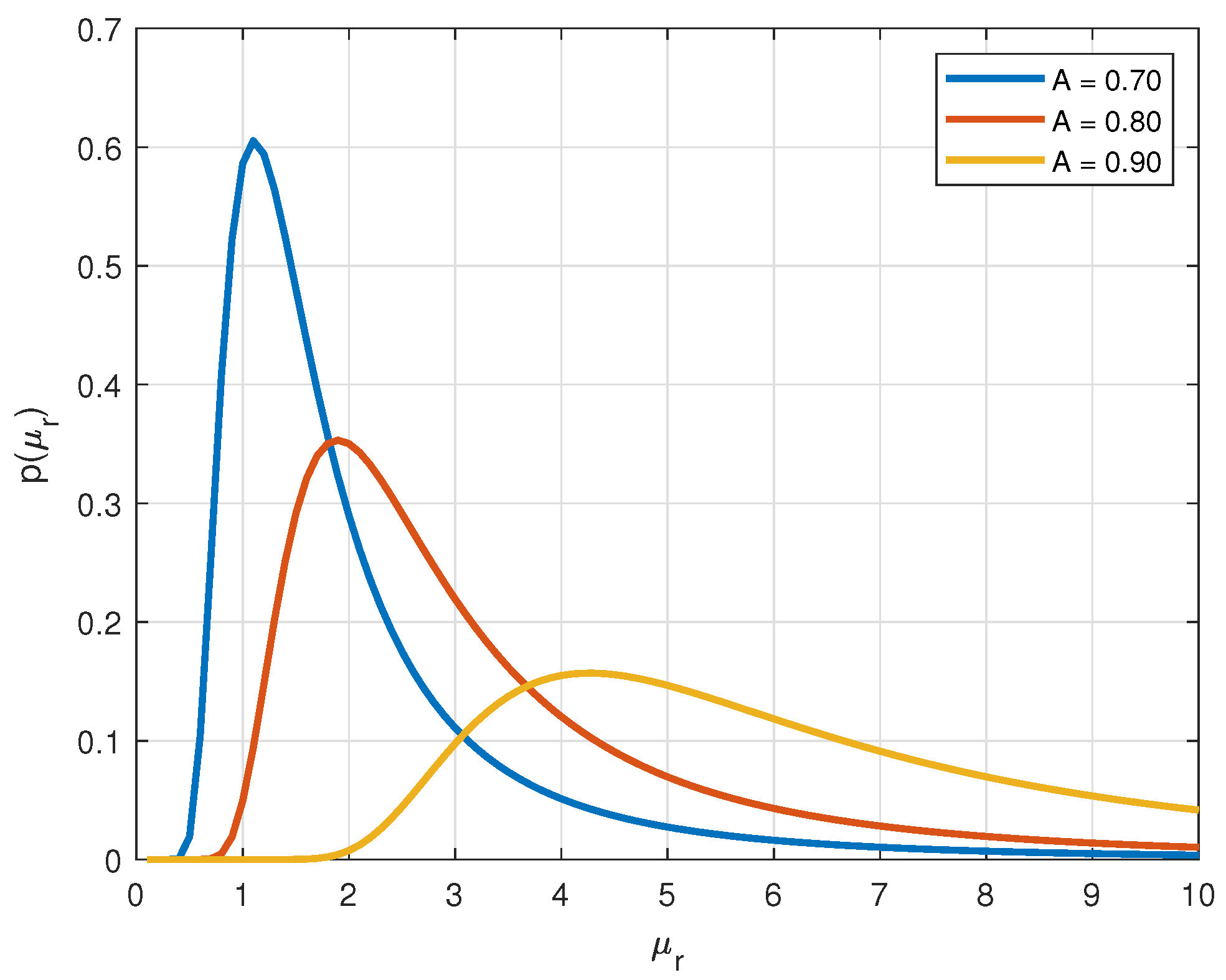
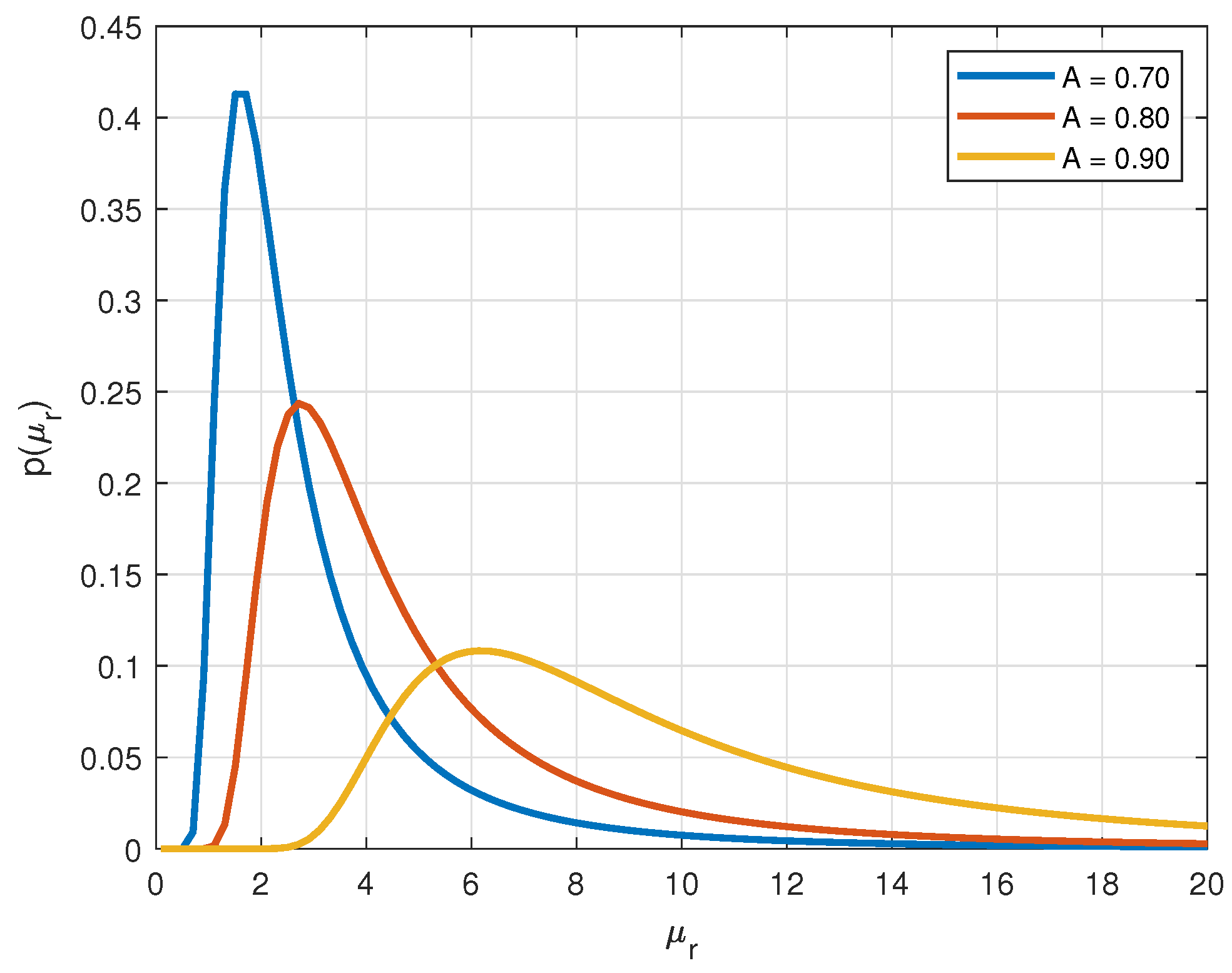
The PDF plots illustrate the probability distribution of repair rates, showing how system availability affects the required maintenance efforts. As can be noticed from Figure 1, Figure 2 and Figure 3, higher availability levels ( A = 0.9 ) lead to a shift in the PDF toward higher repair rates, indicating a need for more frequent and efficient maintenance interventions. Lower availability levels ( A = 0.7 and A = 0.8 ) allow for broader distributions, where lower repair rates remain more probable. Components with higher failure rates (0.84) exhibit a more narrow and peaked PDF, meaning that their repair rates are more predictable and concentrated within a certain range.
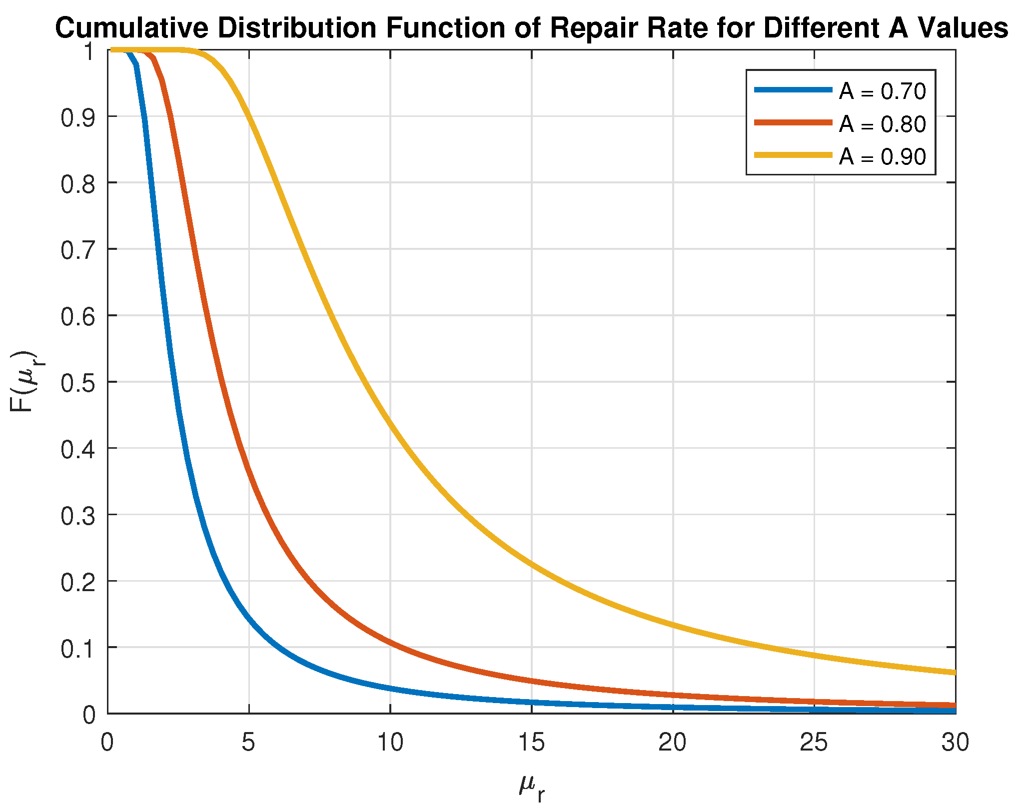
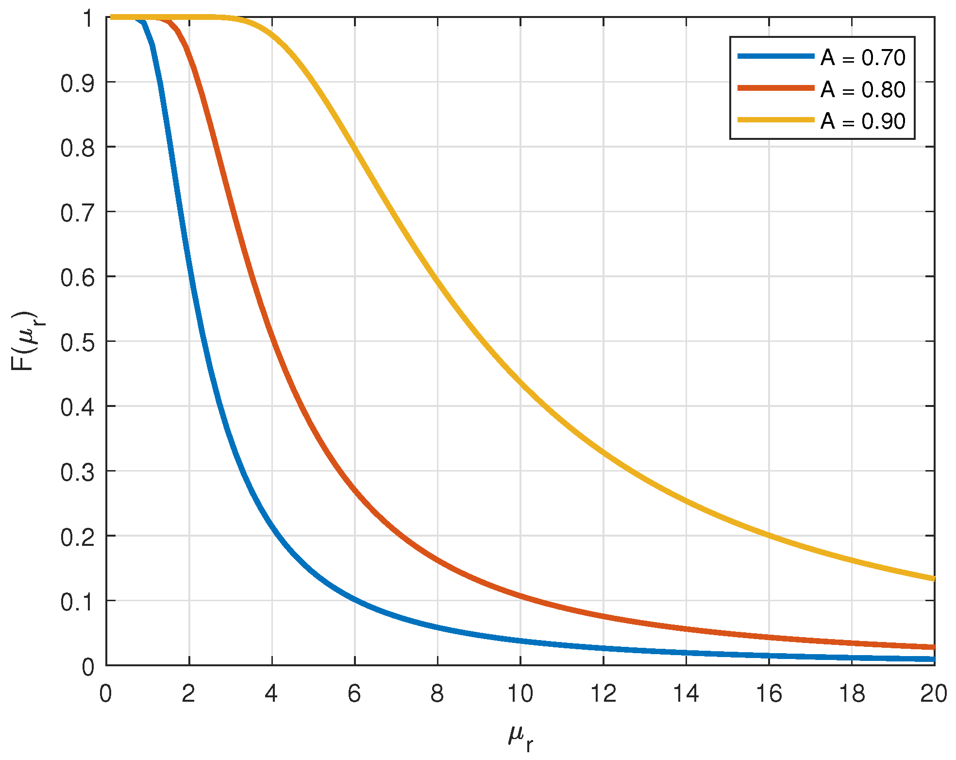
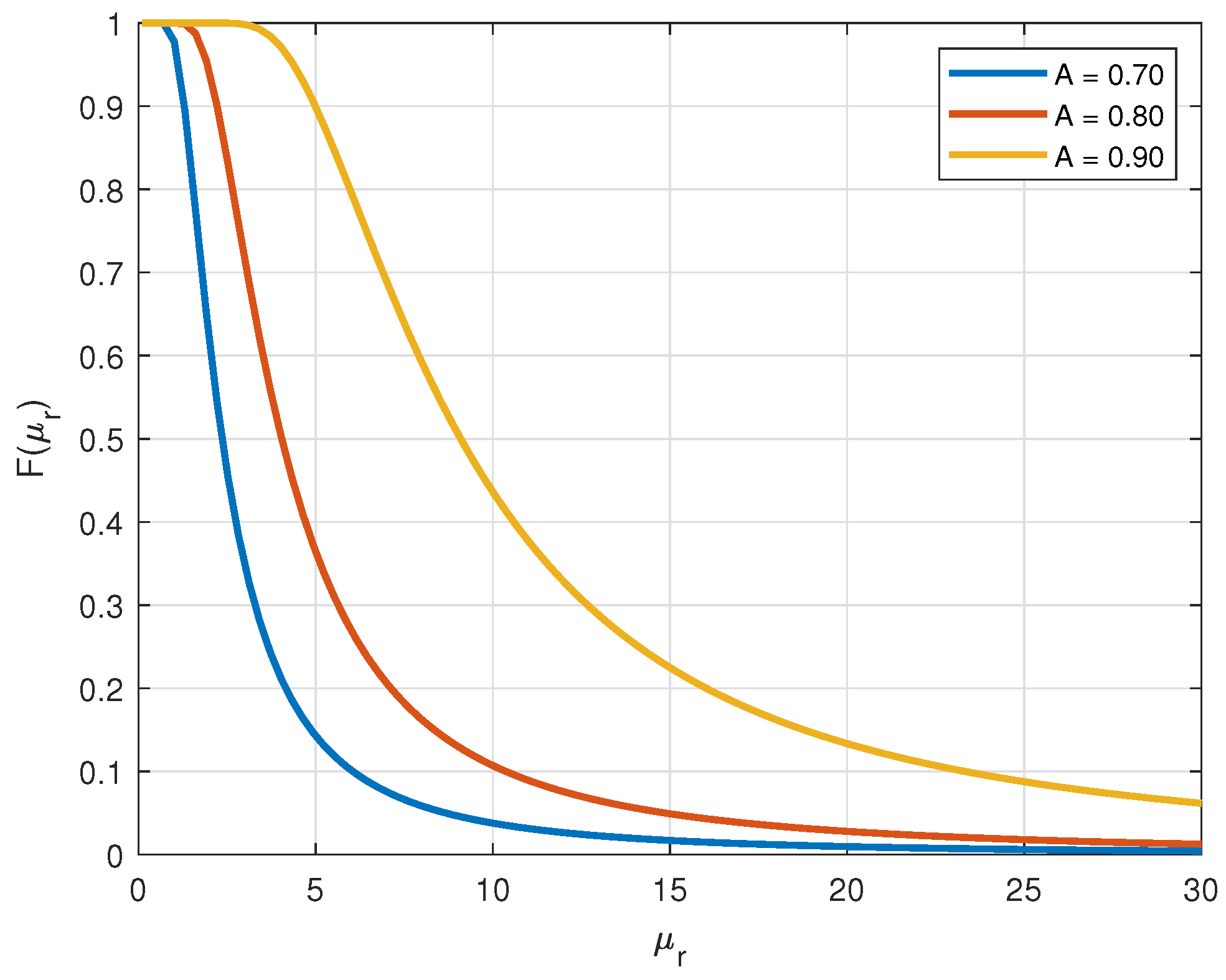
The CDF plots provide insight into the cumulative probability of the repair rate being below a certain threshold. Steeper CDF curves for A = 0.9 suggest that high repair rates are required with greater certainty, as maintaining high availability imposes strict maintenance requirements. More gradual CDF curves for A = 0.7 and A = 0.8 indicate that lower repair rates are more common, reducing the intensity of required maintenance interventions. Across all cases, higher failure rates result in steeper CDFs, confirming that more frequent repairs are essential for components with high failure probabilities. These are presented in Figure 4, Figure 5 and Figure 6.
The numerical results confirm that the stochastic model accurately predicts repair rate distributions under different operating conditions. Specifically, higher failure rates necessitate higher repair rates, validating the theoretical assumptions of the model. Increased availability constraints shift the repair rate distributions, aligning with expectations that greater availability requires more proactive maintenance. PDF and CDF trends follow standard probabilistic behavior, demonstrating the reliability of the model in estimating repair rates. The numerical analysis supports the effectiveness of the stochastic model in predicting repair rate distributions for different system configurations. The results confirm that both failure rates and availability levels significantly impact repair rate requirements, reinforcing the applicability of the model in predictive maintenance planning and logistics optimization. This validation further strengthens the case for integrating machine learning techniques to enhance repair rate estimations and automate maintenance decision-making.
To further support predictive maintenance strategies, extreme values such as maximum and minimum repair rates are also computed. The maximum repair rate x max = max ( μ r 1 , μ r 2 , , μ r n ) and minimum repair rate x min = min ( μ r 1 , μ r 2 , , μ r n ) play a crucial role in evaluating the robustness and efficiency of repair processes in PBL systems. These extreme values provide insights into the best-case and worst-case repair scenarios, which are essential for risk assessment, maintenance scheduling, and predictive modeling. The minimum repair rate x min represents the longest expected repair duration, corresponding to situations where system recovery is slow due to operational constraints, resource limitations, or unexpected failures. This value helps in defining worst case maintenance scenarios and ensuring that systems remain operational even under adverse conditions. Conversely, the maximum repair rate x max represents the shortest expected repair time, which is important for identifying optimal maintenance conditions and achievable system recovery performance. By analyzing x max , maintenance planners can assess whether a given system meets contractual availability targets and optimize maintenance resource allocation. By considering both x max and x min , decision-makers can establish realistic repair time expectations, optimize maintenance cycles, and design predictive maintenance strategies that account for variability in repair durations, ultimately enhancing system reliability and operational efficiency. In [9] a novel method for the determination of the maximum and minimum repair rates of the entity comprising the observed units is presented. The obtained generalized PDF expressions can be used to predict total repair time. The presented method provides two new measures that comprehensively define the total repair time and have not been studied in this way before. In the numerical section, the proposed model was applied to the before mention system consisting of three key components. PDFs of repair rate for each component, as well as the PDF and CDF maximum and minimum repair rates for the entire system. In this case selection of three random variables ( μ r 1 , μ r 2 , μ r 3 ) for computing the maximum and minimum repair rates is based on the practical constraints of system redundancy and maintenance decision-making. Many real-world systems operate with a limited number of redundant components or subsystems (typically three or fewer), where each component undergoes independent repair processes under varying operational conditions. Observing a higher number of random variables would increase computational complexity without significantly improving the accuracy of repair rate estimation, as beyond a certain threshold, additional components contribute diminishing returns in predictive maintenance optimization. To accurately model the stochastic nature of the system repair rate, we implement a sampling-based approach that generates random repair rate samples for different system availabilities A 1 , A 2 , A 3 . This process enables us to analyze the variability in repair rate estimations under different operational conditions. Given the system parameters representing different component characteristics, and availability levels A 1 , A 2 , A 3 , the repair rate samples are computed separately for different components of the system, resulting in three vectors of repair rate realizations: μ r 1 = [ μ 11 , μ 12 , μ 13 ] , μ r 2 = [ μ 21 , μ 22 , μ 23 ] , μ r 3 = [ μ 31 , μ 32 , μ 33 ] , where each vector represents repair rates for different configurations of system availability. To analyze the best-case and worst-case scenarios, we compute the minimum and maximum repair rates across the three sampled vectors:
x min = min ( μ r 1 , μ r 2 , μ r 3 )
and
x max = max ( μ r 1 , μ r 2 , μ r 3 )
These computations provide insight into the lower and upper bounds of repair rate estimates under varying operational conditions, ensuring robust predictive maintenance planning.
The obtained stochastic repair rate samples, including their minimum and maximum values, serve as the foundation for training data in the subsequent NN analysis. By connecting the analytical framework of the stochastic model with data-driven predictive modeling, this approach enables efficient estimation of repair rates under varying operational conditions. The following subsection introduces the NN architectures developed for this purpose.

2.2. Neural Network Architecture

An empirical inspection of the simulated repair rate samples confirms the rationale for employing two separate neural models. Maximum repair rate values tend to cluster around their upper stochastic limits and vary smoothly, without exhibiting sequential irregularities, therefore a feed-forward FCNN is sufficient for capturing their steady state behavior. Minimum repair-rate values, however, display pronounced local fluctuations and occasional abrupt drops, making their prediction more sensitive to short-term variations. Such fluctuation patterns are more effectively handled by an LSTM architecture, which is designed to model irregular or context dependent changes across adjacent samples even when the overall sequence is not strongly time dependent.
Building on the stochastic model results, two NN architectures were developed to predict repair rates more efficiently and adaptively. The generated repair rate samples were used as inputs, allowing the networks to learn complex nonlinear relationships between system availability and repair performance.
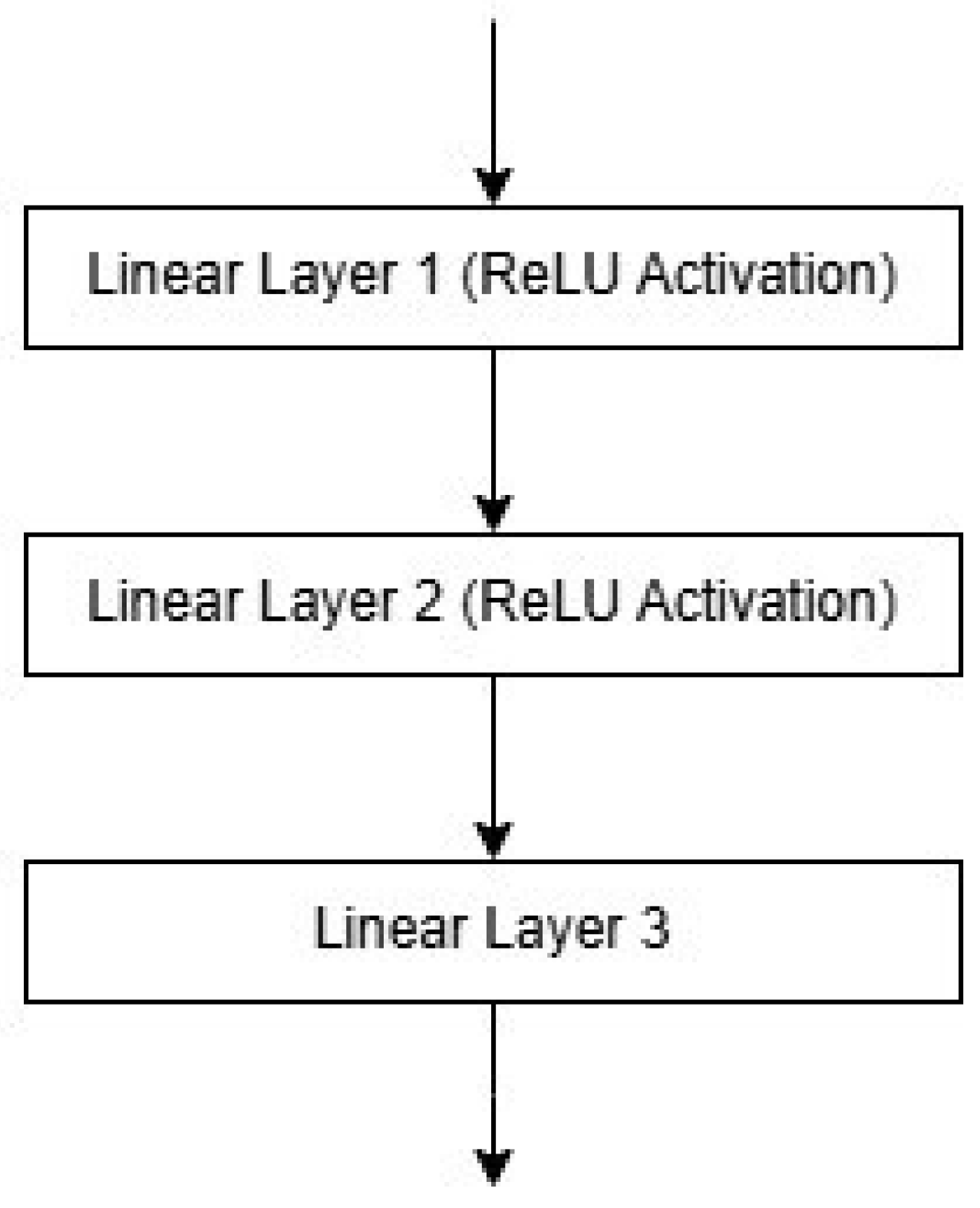
The first model is an FCNN, designed to predict the maximum repair rates ( x 1 m a x , x 2 m a x , x 3 m a x ) based on nine input features. Its architecture, shown in Figure 7, consists of three fully connected (linear) layers. The first layer comprises 128 neurons, the second layer 64 neurons, while the output layer contains three neurons responsible for predicting the target values. Each hidden layer utilizes the Rectified Linear Unit (ReLU) activation function, which facilitates efficient learning of nonlinear relationships in the data. The ReLU activation function is defined as follows [18]:
ReLU ( z ) = max ( 0 , z )
where z is the input to the neurons. This model is well-suited for regression tasks since the output layer does not employ an activation function, allowing for continuous value predictions. The network is trained using the Mean Squared Error (MSE) loss function, which minimizes the squared differences between the actual and predicted values. In addition to the MSE loss function, other metrics were used to further evaluate the model’s performance: Mean Absolute Error (MAE), Root Mean Squared Error (RMSE), and the coefficient of determination (R-squared). MAE measures the average absolute prediction error, while RMSE emphasizes larger errors by penalizing them through squaring. R-squared assesses how well the model explains the variability in the data, with values closer to 1 indicating better model fit.
To improve training stability, batch normalization was also tested after each fully connected layer. This technique normalizes activations across mini-batches, reducing internal covariant shift and allowing for higher learning rates [19]. However, the results did not improve as expected, and in some cases, performance slightly degraded. Therefore, batch normalization was ultimately not included in the final model configuration.
The optimization of parameters is performed using the Adaptive Moment Estimation (Adam) algorithm with an initial learning rate of 0.001 and L2 regularization (weight decay) of 10 4 , which helps mitigate overfitting. Adam combines the benefits of momentum and adaptive learning rates, enabling more stable and efficient convergence [20].
Before training, all input data were standardized using the Standard Scaler (SS) method to avoid feature imbalance and accelerate convergence. This transformation ensures that the data have a zero mean and unit standard deviation, facilitating faster and more efficient model learning. The transformation is performed using the formula:
x * = x μ σ
where μ and σ represent the mean and standard deviation of each feature, respectively [21].
The dataset was divided into training and testing subsets, with 80% used for model fitting and 20% reserved for performance evaluation. This ensured objective validation of the model’s generalization capability.
To ensure a fair comparison between the proposed neural networks and the stochastic baseline estimators, all models were evaluated using the exact same simulation samples and under identical computational conditions. The stochastic MLE estimators and both neural architectures were exposed to the same number of repair rate realizations, identical Rayleigh parameter distributions, and consistent runtime constraints. This guarantees that any observed differences in performance arise solely from methodological effectiveness rather than dataset variation or computational advantage.

3. Results and Discussion

In this study, both FCNN and the LSTM NN demonstrated excellent performance in estimating the maximum and minimum repair rates, respectively. The performance of these NNs was evaluated across various configurations by modifying the optimizer, the number of neurons, and the learning rate. Four optimization algorithms were considered: Adam, SGD, RMSprop, and Adagrad. Experiments were conducted with network architectures consisting of 64, 128, and 256 neurons. For the FCNN, the learning rates were set to 0.01, 0.001, and 0.0001, whereas for the LSTM network, they were adjusted to 0.025, 0.0025, and 0.00025. The initial training and validation were performed on a dataset containing 10,000 samples, followed by further evaluations on larger datasets with 100,000 and 1,000,000 samples to assess the generalization capability of the models. In the case of the FCNN, the Adam optimizer exhibited the best overall performance across all tested configurations. This was evident from its consistently lower MSE, MAE, and RMSE values, as well as its higher R-squared score compared to the other optimizers. Adam’s ability to adapt learning rates dynamically for each parameter allowed it to converge more efficiently while avoiding the pitfalls of suboptimal local minima. In contrast, SGD and RMSprop struggled with convergence stability, and Adagrad, while performing reasonably well, exhibited slower learning behavior, particularly in later training stages. These findings indicate that Adam provides a well-balanced combination of stability and rapid convergence, making it the most suitable optimizer for training the FCNN model in this study. The results of this analysis are summarized in Table 2, which presents the performance metrics obtained for different optimizers.
To further improve the performance of the FCNN, the impact of batch normalization and L2 regularization was investigated. The Adam optimizer was selected as the baseline, given its superior performance in the previous analysis. The analysis included four configurations: with batch normalization and L2 regularization, with batch normalization and without L2 regularization, without batch normalization and with L2 regularization, and without both batch normalization and L2 regularization. The results of this comparison are presented in Table 3.
Among these configurations, the best performance was observed in the model trained without batch normalization but with L2 regularization. This suggests that L2 regularization effectively prevents overfitting by penalizing large weights, leading to a more stable and generalizable model. On the other hand, batch normalization did not contribute significantly to performance improvement in this specific case, possibly due to the fully connected network structure and the nature of the dataset. These results indicate that, for the FCNN, L2 regularization should be prioritized over batch normalization when optimizing model performance. Consequently, best configuration for the FCNN model was found to be without batch normalization but with L2 regularization, achieving near perfect R-squared values and the lowest error metrics. The unexpectedly poor performance of batch normalization at 100 epochs may suggest that early-stage normalization disrupts stable weight updates, while its lack of effectiveness at 400+ epochs indicates that L2 regularization alone is sufficient to prevent overfitting. These findings reinforce that batch normalization is not always beneficial in deep learning models and that its impact should be carefully evaluated depending on the architecture and training conditions.
After determining that Adam was the best-performing optimizer, further optimization was conducted by analyzing the impact of different learning rates (0.01, 0.001, and 0.0001) across networks with 64, 128, and 256 neurons. The results confirm that Adam consistently produced superior performance across all configurations. Specifically:
  • Learning rates of 0.01 and 0.001 yielded excellent results, with MSE values close to zero and R-squared = 1.0000, indicating near perfect model accuracy.
  • A learning rate of 0.0001 significantly degraded performance, leading to higher MSE, MAE, and RMSE values, along with reduced R-squared scores. This suggests that the learning rate was too small, preventing the model from converging efficiently.
  • Networks with 128 and 256 neurons achieved the best results, particularly at lr = 0.01 and lr = 0.001, where the error metrics were minimal and R-squared remained at 1.0000.
While SGD and RMSprop also performed well, their results were slightly less consistent than Adam’s. In contrast, Adagrad showed poor generalization, with negative R-squared values at lr = 0.0001 for 128 and 256 neurons, indicating a failure to capture meaningful relationships in the data, likely due to its aggressive learning rate decay, which prevents effective weight updates. These findings further confirm that Adam, with a learning rate of 0.01 or 0.001, is the most suitable choice for training the FCNN. The complete results of this analysis are summarized in Table 4. The results confirm that Adam is the most effective optimizer, achieving near-perfect performance across all configurations. While SGD improves with more training and larger networks, RMSprop shows inconsistent results, suggesting that it is highly sensitive to hyperparameters. These findings highlight the importance of careful optimizer selection and hyperparameter tuning to ensure model stability and convergence.
To verify the generalization capability of the NN, the best-performing configuration—Adam optimizer with and without batch normalization and L2 regularization—was evaluated on larger datasets containing 100,000 and 1,000,000 samples. The objective was to determine whether the optimal training conditions observed on 10,000 samples would scale effectively to more extensive datasets. The results reaffirmed previous findings:
  • Networks trained without batch normalization and with L2 regularization (weight decay) consistently achieved the best performance, maintaining low MSE, MAE, and RMSE values, while preserving an R-squared value close to 1.0000. Batch normalization did not improve accuracy on larger datasets and, in some cases, led to slightly worse generalization performance. This suggests that for this specific problem, batch normalization does not provide a significant advantage and may even introduce unnecessary variance.
  • Increasing the dataset size improved model stability, reducing variability in performance across different training runs. This confirms that the selected model configuration scales effectively and maintains robustness even with significantly larger datasets.
These findings indicate that L2 regularization is essential for preventing overfitting, especially as dataset size increases, while batch normalization does not contribute to performance improvements in this case. The detailed results of this evaluation are provided in Table 5.
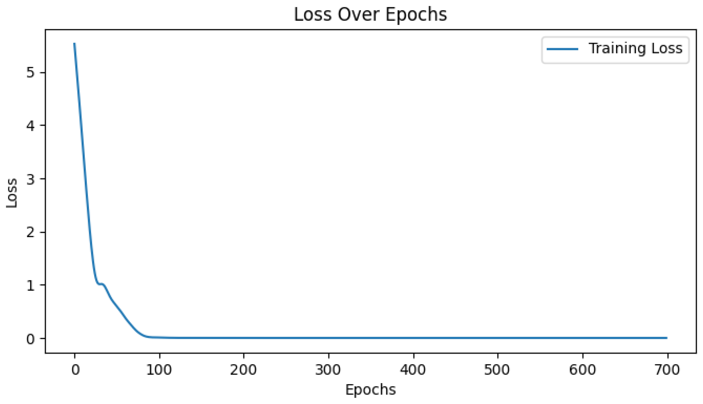
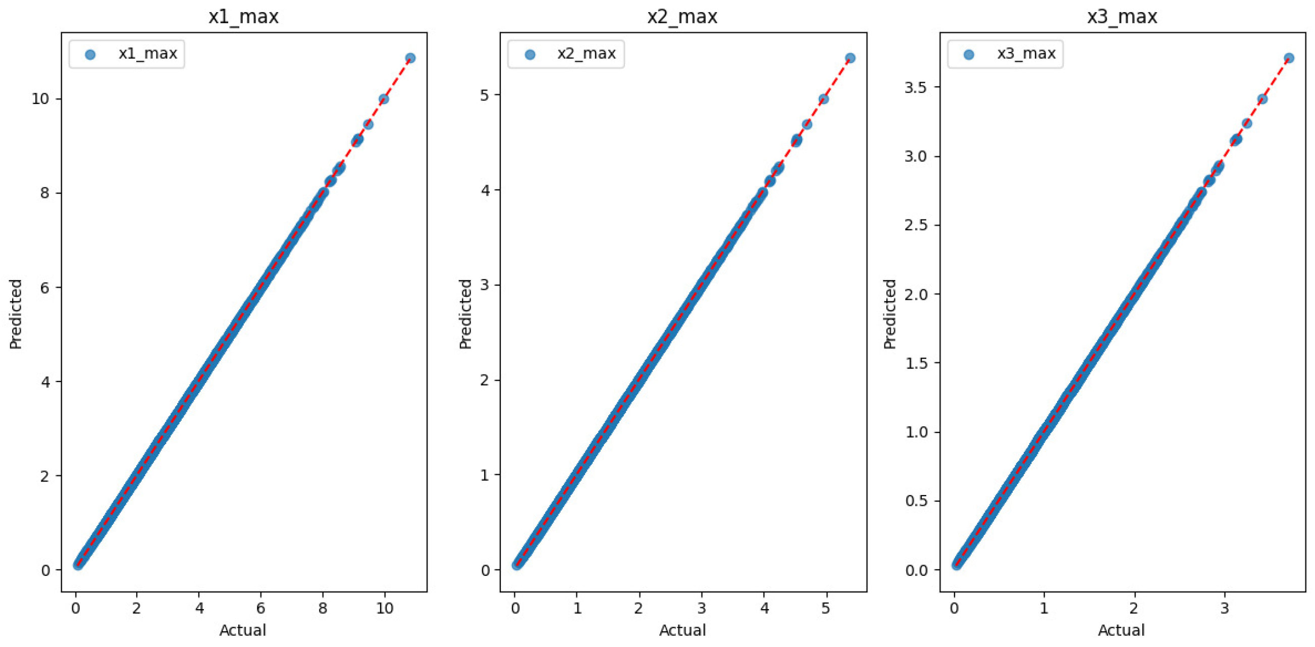
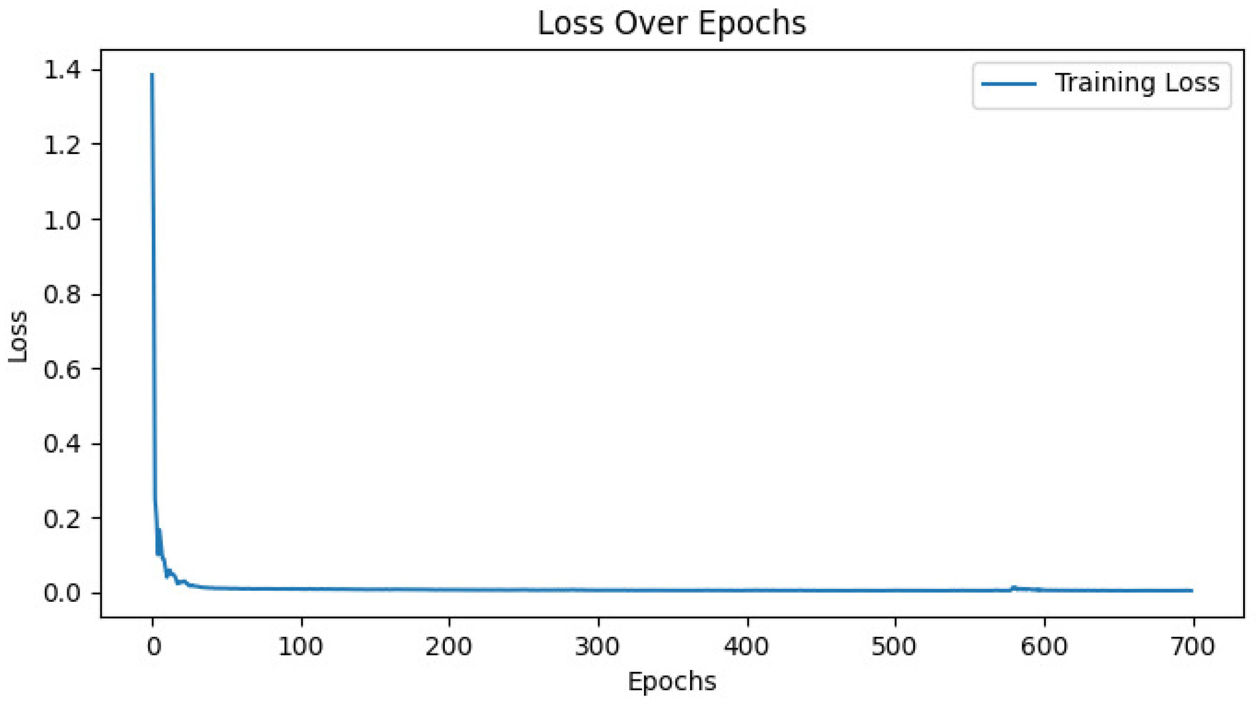
The results were excellent, and determining the best model was challenging due to the similar performance across configurations. The optimal model utilized the Adam optimizer, a learning rate of 0.01 (as seen in Test 31, Test 32, and Test 33, where the MSE is almost 0 and R-squared is nearly 1), with L2 regularization and no batch normalization, trained for 700 epochs on datasets of 10,000 samples. Additionally, the model with 128 neurons produced slightly better results compared to the 256-neuron configuration for all optimizers and learning rates tested. The loss throughout the epochs is shown in Figure 8, illustrating the convergence pattern of the training loss. The training loss decreases rapidly at the beginning, demonstrating the model’s ability to efficiently learn from the training data. Interestingly, the combination of batch normalization with L2 regularization resulted in slightly higher MSE at 100,000 samples, suggesting that early-stage weight normalization may introduce additional variance. However, as the dataset size increases to 1M samples, all configurations achieve near-perfect R-squared values (1.0000), demonstrating that larger datasets enhance model stability and generalization. These findings reinforce that L2 regularization should be prioritized over batch normalization in FCNN for predictive maintenance applications. In Figure 9, a comparison between the true and predicted values is displayed, highlighting how closely the model’s predictions align with the actual values after training. This comparison emphasizes the model’s performance and its capacity to generalize effectively to unseen data. For the LSTM network, similar to the FCNN, various configurations were tested to assess the impact of optimizers, number of neurons, learning rates, and regularization techniques. The performance of the LSTM network was evaluated with the same four optimizers (Adam, SGD, RMSprop, and Adagrad) and with different network architectures, including 64, 128, and 256 neurons. The learning rates were set to 0.025, 0.0025, and 0.00025 to explore the effect of different step sizes during training.
The Adam optimizer again yielded the best performance across all tested configurations for the LSTM network. Its ability to adapt the learning rate dynamically for each parameter resulted in fast convergence, while also maintaining stability during the training process. Adam showed consistently lower MSE, MAE, and RMSE values, as well as higher R-squared scores, compared to other optimizers. This performance pattern was observed across various combinations of neurons and learning rates, reinforcing the findings from the FCNN analysis. In contrast, SGD and RMSprop showed less stability in terms of accuracy, while Adagrad, although performing reasonably well, faced challenges in some configurations. The results of this analysis are summarized in Table 6. SGD performs significantly worse at 100 epochs, with an MSE of 0.2485 and an R-squared value of only 0.0967, indicating that it requires longer training times to converge properly. Interestingly, Adagrad starts with higher error values at 100 epochs but improves significantly over longer training durations, suggesting that it benefits from extended training cycles but struggles in early learning stages. These findings highlight the importance of selecting optimizers based on training duration, with Adam providing the best balance of convergence speed and accuracy for this predictive maintenance application.
Next, the impact of regularization techniques was examined for the LSTM network. The results indicated that the best performance was achieved in the configuration without batch normalization and without L2 regularization, as shown in Table 7. This configuration demonstrated the lowest error metrics (MSE, MAE, and RMSE) and maintained high R-squared values, suggesting that for this specific task, L2 regularization and batch normalization did not contribute significantly to improving performance. While L2 regularization often helps prevent overfitting, its effect was not as pronounced in the LSTM model as it was in the FCNN. Additionally, batch normalization did not provide a noticeable improvement in generalization for the LSTM network, supporting the conclusion that it is not always beneficial for every type of network architecture. The best configuration was found to be without batch normalization and without L2 regularization, achieving the lowest MSE and highest R-squared values. Surprisingly, batch normalization combined with L2 regularization resulted in the highest error values at 100 epochs, suggesting that batch normalization interferes with the sequential nature of LSTMs, disrupting information flow between time steps. Additionally, L2 regularization appears to be less effective for LSTMs than for FCNNs, likely because LSTMs already include internal mechanisms (gates) that regulate weight updates and prevent overfitting. These findings highlight that regularization techniques that work well for FCNNs may not necessarily benefit recurrent architectures like LSTMs.
The optimal results for the LSTM model were achieved using the Adam optimizer with a learning rate of 0.025, no batch normalization, and no L2 regularization. Networks with 128 neurons produced the best results, yielding minimal errors and maintaining a near-perfect R-squared score. These findings are summarized in Table 8. Adam is the best optimizer for LSTM networks, achieving the lowest MSE and highest R-squared values across different learning rates and network sizes. SGD performs poorly at low learning rates, indicating that it does not adapt well to the sequential nature of LSTMs without momentum tuning. Adagrad completely fails at lr = 0.00025, showing negative R-squared values due to excessive learning rate decay, which causes the model to stop learning. RMSprop exhibits inconsistent behavior, performing well in some cases but struggling in others, suggesting that it requires precise tuning for effective LSTM training. These findings highlight that Adam provides the best balance of stability and performance, while other optimizers require careful tuning to be effective.
Overall, these results confirm the superiority of the Adam optimizer for training both FCNN and LSTM models, highlighting its efficiency in handling various architectures and learning rates. Additionally, for the LSTM network, the absence of batch normalization and L2 regularization proved to be the most effective configuration, aligning with the findings from the FCNN model. The results for the larger datasets of 100,000 and 1,000,000 samples are summarized in Table 9, where the metric values show consistency with those achieved using the 10,000 sample dataset, further validating the model’s robust generalization capabilities. LSTM models perform best without batch normalization and L2 regularization, with near-zero error metrics across configurations. The slightly higher MSE for batch normalization + L2 regularization at 100,000 samples suggests that batch normalization disrupts temporal learning in LSTMs, while L2 regularization adds little benefit due to the model’s built-in gating mechanisms. However, as the dataset size increases to 1M samples, all configurations achieve near-perfect R-squared values (1.0000), demonstrating that large datasets enhance model stability and reduce the need for additional regularization techniques.
Figure 10 depicts the loss across epochs, highlighting the convergence trend of the training loss. In Figure 11, a comparison of the true and predicted values for the minimum repair rates is presented, showcasing how accurately the LSTM model predicts the actual values after training.
The sensitivity analysis presented in Table 10 illustrates the behavior of both the FCNN and LSTM models under different values of the availability parameter A. By varying A values across three representative scenarios, we observe that the prediction accuracy of both models remains stable for observed availability levels, with performance degradation becoming noticeable only for extreme values. These findings confirm that the models are robust to variations in system availability and therefore well suited for practical implementation in environments where operational conditions may fluctuate. Furthermore, the comparative behavior across architectures provides empirical justification for the modeling choices: while the FCNN performs reliably in non-sequential settings, the LSTM yields superior accuracy in regimes where temporal dependencies within repair-rate sequences play a significant role.
In addition to accuracy metrics, Table 10 reports the corresponding training times and convergence epochs, offering a clear view of the computational feasibility of the proposed approach. The FCNN achieves faster convergence due to its feed-forward structure, whereas the LSTM requires longer training times as a consequence of its recurrent gating operations. Despite this difference, both models maintain execution times compatible with real-time predictive maintenance scenarios, confirming their suitability for deployment in practical environments. This analysis demonstrates that the proposed NNs generalize consistently across varying availability conditions without signs of overfitting, and it provides further justification for selecting FCNN and LSTM architectures as efficient and scalable alternatives to classical stochastic estimators.
Compared with classical Monte Carlo estimation, whose convergence requires a large number of samples, and Bayesian methods that rely on explicit likelihood updates, the proposed neural architectures deliver instant predictions and bypass the need for iterative probabilistic inference. This makes them highly suitable as fast surrogate estimators for real-time repair rate prediction in maintenance planning systems.
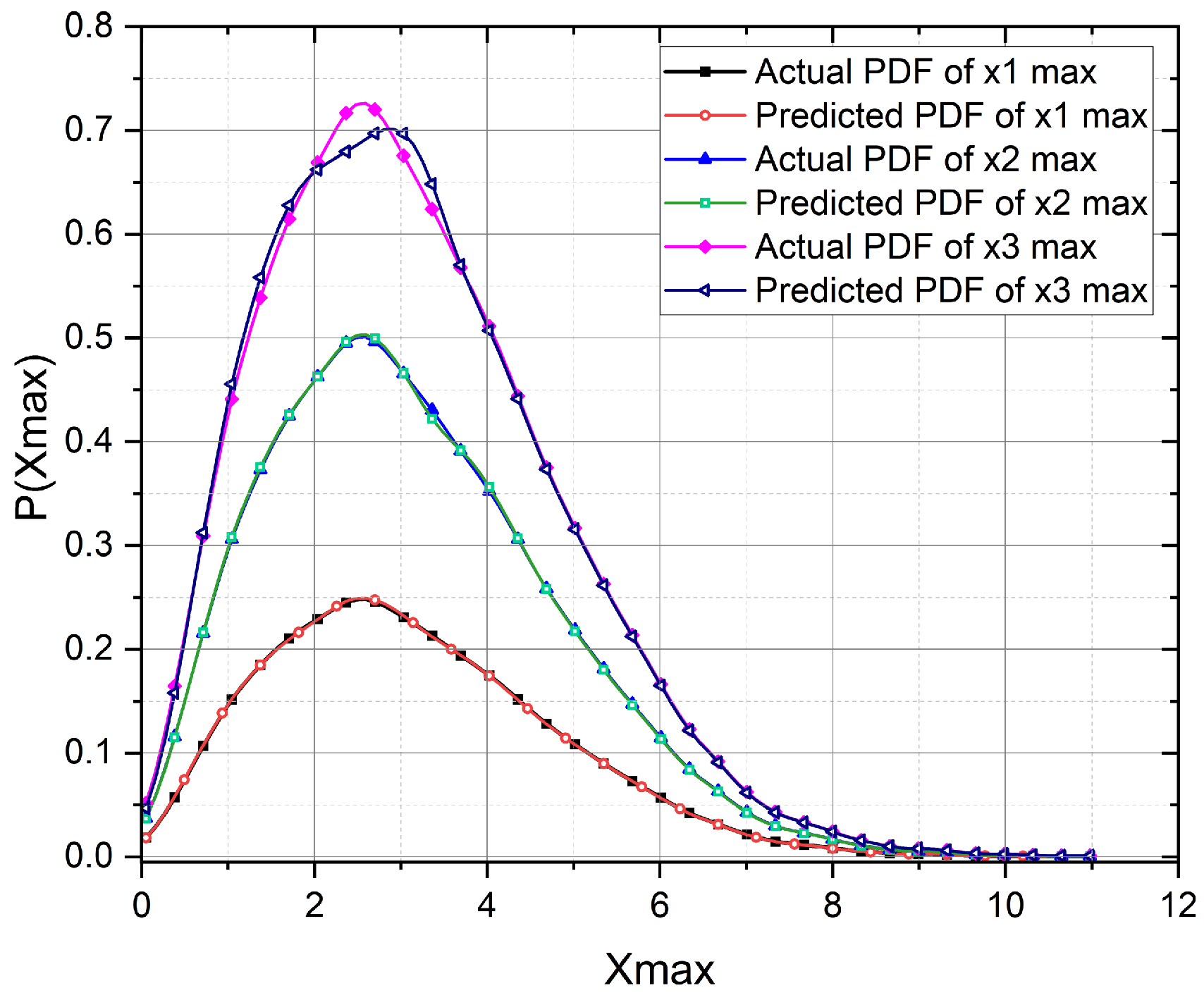
Figure 12 and Figure 13 illustrate the comparison between the actual and predicted PDFs for maximum and minimum repair rates, respectively. These graphs demonstrate the effectiveness of the proposed NN-based optimization approach in estimating repair rate distributions within a performance-based logistics system. In Figure 12, the predicted PDF closely follows the actual PDF for maximum repair rates, indicating a high level of accuracy in capturing the underlying distribution of the data.
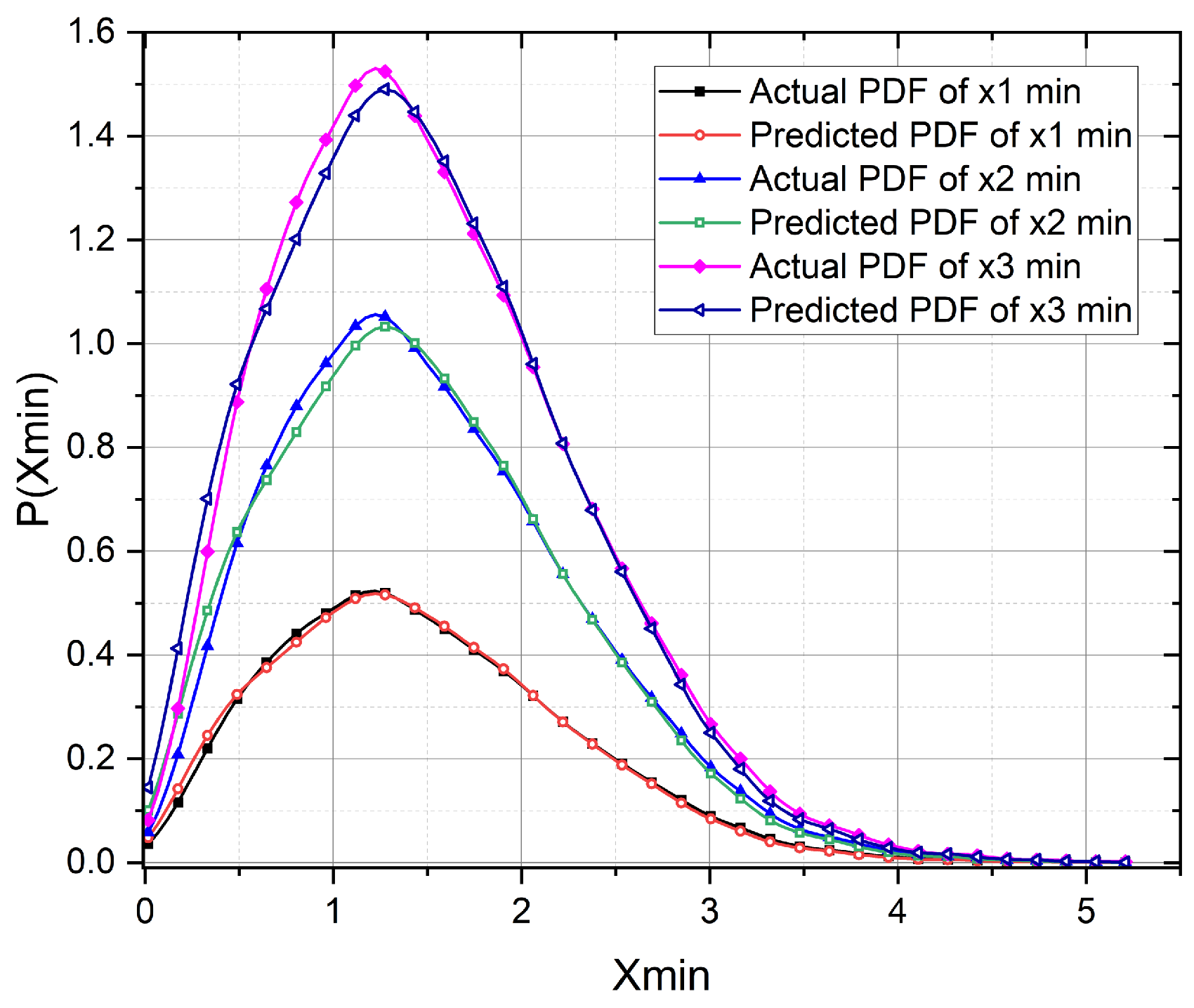
Similarly, Figure 13 presents the comparison for minimum repair rates, showing a strong alignment between predicted and actual values. The minor deviations observed in both graphs suggest that the model effectively generalizes across different repair rate scenarios while maintaining a low error margin. These results confirm that the NN-based approach is capable of accurately estimating repair rate distributions, making it a reliable tool for predictive maintenance and logistics optimization.

4. Conclusions and Future Work

This paper presents a novel NN-based framework for repair rate estimation in PBL systems, bridging the gap between traditional stochastic modeling and modern data-driven predictive maintenance. By training FCNN and LSTM networks on repair rate samples generated from a stochastic model, the framework offers a computationally efficient and flexible alternative to traditional analytical formulations. Unlike conventional analytical approaches, the proposed method eliminates the need for complex mathematical derivations and provides a scalable, real-time solution that can adapt to diverse operational conditions.
The results suggest that both NN architectures achieve high predictive accuracy, with low error metrics and strong generalization across different dataset sizes and system configurations. The FCNN is effective in modeling maximum repair rates, while the LSTM captures sequential patterns associated with minimum repair rates. Together, these architectures demonstrate that deep learning can replicate and surpass the performance of analytical estimators while drastically reducing computation time, which is critical for real-time repair planning and predictive maintenance applications. These findings indicate that deep learning provides a promising complement to conventional stochastic approaches by reducing computational complexity and enabling near-real-time estimation capabilities.
The primary strengths of this study lie in its integration of reliability engineering principles with advanced AI architectures and its demonstration of strong scalability across multiple availability scenarios. The predicted repair rates offer direct utility in scheduling maintenance interventions, planning spare parts inventory, and managing system availability. By leveraging the predictive precision and fast inference of FCNN and LSTM models, maintenance planners can improve decision-making, minimize downtime, and optimize resource allocation, leading to measurable cost and time efficiencies. In addition to performance improvements, this research demonstrates the potential of integrating machine learning with reliability engineering to support predictive maintenance decision-making within PBL frameworks. The models’ adaptability and scalability make them suitable candidates for deployment in maintenance planning and logistics optimization. Across all tested availability scenarios, the FCNN and LSTM architectures consistently achieved higher predictive accuracy and superior numerical stability relative to the stochastic baseline, confirming the practical advantages of data-driven estimation methods.
The present study intentionally employs a minimal feature set composed solely of repair rate samples in order to isolate and evaluate the predictive capabilities of the proposed neural architectures without confounding effects from auxiliary variables. This controlled environment enabled a transparent and rigorous comparison between classical stochastic estimators and the proposed neural models. While this provides a clean and controlled benchmark, future work could benefit from expanding the input space to include operational, environmental, and condition monitoring variables, enabling richer feature representations and improving applicability in real maintenance environments. Further the proposed models could be tested on actual maintenance records through pilot studies within PBL maintenance systems to evaluate real-world applicability and accuracy. Once trained, both architectures are capable of real-time inference, enabling integration into predictive maintenance decision support tools for dynamic repair planning. Future research should therefore incorporate empirical maintenance records to validate the models under realistic conditions and to identify domain-specific patterns not observable in simulations. Such extensions would also facilitate the development of hybrid neural–stochastic frameworks that combine the interpretability of analytical models with the predictive power demonstrated by deep learning in this study.

Author Contributions

M.D., S.P., N.K., D.Đ. and S.M. contributed equally to the conceptualization, methodology, investigation, and writing of this manuscript. All authors have read and agreed to the published version of the manuscript.

Funding

The authors gratefully acknowledge the support from the Serbian Ministry of Science, Technological Development and Innovation (Contract No. 451-03-65/2024-03/200123).

Institutional Review Board Statement

Not applicable.

Informed Consent Statement

Not applicable.

Data Availability Statement

The datasets generated and analyzed during the current study are available from the corresponding author on reasonable request.

Conflicts of Interest

The authors declare no conflicts of interest.

References

  1. Kontrec, N.; Panić, S.; Petrović, M.; Milošević, H. A Stochastic Model for Estimation of Repair Rate for System Operating under Performance-Based Logistics. Ekspl. Niezawodn.—Maint. Reliab. 2018, 20, 68. [Google Scholar] [CrossRef]
  2. Milković, V.; Osman, K.; Jankovich, D. Reliability-Based Model for Optimizing Resources in the Railway Vehicles Maintenance. Mech. Eng. J. 2024, 11, 24–00070. [Google Scholar] [CrossRef]
  3. Numsong, A.; Posom, J.; Chuan-Udom, S. Artificial Neural Network-Based Repair and Maintenance Cost Estimation Model for Rice Combine Harvesters. Int. J. Agric. Eng. Technol. 2023, 16, 38–47. [Google Scholar] [CrossRef]
  4. Ouadah, A.; Zemmouchi-Ghomari, L.; Salhi, N. Selecting an Appropriate Supervised Machine Learning Algorithm for Predictive Maintenance. Int. J. Adv. Manuf. Technol. 2022, 119, 4277. [Google Scholar] [CrossRef]
  5. Dhada, M.; Parlikad, A.K.; Steinert, O.; Lindgren, T. Weibull Recurrent Neural Networks for Failure Prognosis Using Histogram Data. Neural Comput. Appl. 2022, 35, 3011. [Google Scholar] [CrossRef]
  6. Kontrec, N.; Panić, S.; Panić, B.; Marković, A.; Stošović, D. Mathematical Approach for System Repair Rate Analysis Used in Maintenance Decision Making. Axioms 2021, 10, 96. [Google Scholar] [CrossRef]
  7. Sharma, J.; Mittal, M.L.; Soni, G. Condition-Based Maintenance Using Machine Learning and the Role of Interpretability: A Review. Int. J. Syst. Assur. Eng. Manag. 2024, 15, 1345. [Google Scholar] [CrossRef]
  8. Zhai, S.; Kandemir, M.G.; Reinhart, G. Predictive Maintenance Integrated Production Scheduling by Applying Deep Generative Prognostics Models: Approach, Formulation and Solution. Prod. Eng. 2022, 16, 65. [Google Scholar] [CrossRef]
  9. Jahangard, M.; Xie, Y.; Feng, Y. Leveraging Machine Learning and Optimization Models for Enhanced Seaport Efficiency. Marit. Econ. Logist. 2025, 1–42. [Google Scholar] [CrossRef]
  10. Gu, X.; Han, J.; Shen, Q.; Angelov, P.P. Autonomous Learning for Fuzzy Systems: A Review. Artif. Intell. Rev. 2023, 56, 7549–7595. [Google Scholar] [CrossRef]
  11. Pagano, D. A Predictive Maintenance Model Using Long Short-Term Memory Neural Networks and Bayesian Inference. Decis. Anal. J. 2023, 6, 100174. [Google Scholar] [CrossRef]
  12. Li, Z.; He, Q.; Li, J. A Survey of Deep Learning-Driven Architecture for Predictive Maintenance. Eng. Appl. Artif. Intell. 2024, 133, 108285. [Google Scholar] [CrossRef]
  13. Benhanifia, A.; Ben Cheikh, Z.; Oliveira, P.M.; Valente, A.; Lima, J. Systematic Review of Predictive Maintenance Practices in the Manufacturing Sector. Intell. Syst. Appl. 2025, 26, 200501. [Google Scholar] [CrossRef]
  14. Kim, J.-M.; Yum, S.-G.; Das Adhikari, M.; Bae, J. A LSTM Algorithm-Driven Deep Learning Approach to Estimating Repair and Maintenance Costs of Apartment Buildings. Eng. Constr. Archit. Manag. 2024, 31, 369–389. [Google Scholar] [CrossRef]
  15. Aminzadeh, A.; Sattarpanah Karganroudi, S.; Majidi, S.; Dabompre, C.; Azaiez, K.; Mitride, C.; Sénéchal, E. A machine learning implementation to predictive maintenance and monitoring of industrial compressors. Sensors 2025, 25, 1006. [Google Scholar] [CrossRef] [PubMed]
  16. Li, W.; Li, T. Comparison of Deep Learning Models for Predictive Maintenance in Industrial Manufacturing Systems Using Sensor Data. Sci. Rep. 2025, 15, 23545. [Google Scholar] [CrossRef] [PubMed]
  17. Kontrec, N.; Panić, S.; Panić, B. Availability-Based Maintenance Analysis for Systems with Repair Time Threshold. Yugosl. J. Oper. Res. 2025, 35, 585–593. [Google Scholar] [CrossRef]
  18. Goodfellow, I.; Bengio, Y.; Courville, A. Deep Learning; MIT Press: Cambridge, MA, USA, 2016. [Google Scholar]
  19. Ioffe, S.; Szegedy, C. Batch Normalization: Accelerating Deep Network Training by Reducing Internal Covariate Shift. In Proceedings of the 32nd International Conference on Machine Learning (ICML), Lille, France, 7–9 July 2015; Volume 37, pp. 448–456. [Google Scholar]
  20. Kingma, D.P.; Ba, J. Adam: A Method for Stochastic Optimization. In Proceedings of the 3rd International Conference on Learning Representations (ICLR), San Diego, CA, USA, 7–9 May 2015. [Google Scholar]
  21. Pedregosa, F.; Varoquaux, G.; Gramfort, A.; Michel, V.; Thirion, B.; Grisel, O.; Blondel, M.; Prettenhofer, P.; Weiss, R.; Dubourg, V.; et al. Scikit-Learn: Machine Learning in Python. J. Mach. Learn. Res. 2011, 12, 2825. [Google Scholar]
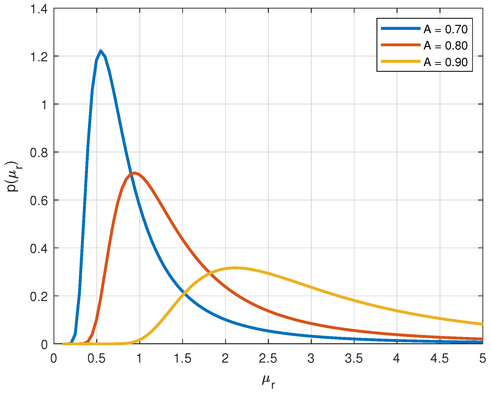
Figure 1. PDF of the repair rate for the first part (failure rate = 0.29).
Information 16 01031 g001
Figure 2. PDF of the repair rate for the second part (failure rate = 0.58).
Information 16 01031 g002
Figure 3. PDF of the repair rate for the third part (failure rate = 0.84).
Information 16 01031 g003
Figure 4. CDF of the repair rate for the first part (failure rate = 0.29).
Information 16 01031 g004
Figure 5. CDF of the repair rate for the second part (failure rate = 0.58).
Information 16 01031 g005
Figure 6. CDF of the repair rate for the third part (failure rate = 0.84).
Information 16 01031 g006
Figure 7. FCNN Architecture.
Information 16 01031 g007
Figure 8. Loss curve during training (700 epochs) for the FCNN model with Adam optimizer and L2 regularization.
Information 16 01031 g008
Figure 9. Comparison of true and predicted values for maximum repair rates.
Information 16 01031 g009
Figure 10. Loss curve during training (700 epochs) for the LSTM model with Adam optimizer.
Information 16 01031 g010
Figure 11. Comparison of true and predicted values for minimum repair rates.
Information 16 01031 g011
Figure 12. Comparison of actual and predicted probability density functions (PDFs) for maximum repair rates.
Information 16 01031 g012
Figure 13. Comparison of actual and predicted probability density functions (PDFs) for minimum repair rates.
Information 16 01031 g013
Table 1. Summary of symbols and abbreviations used in the paper.
Symbol/AbbreviationDescription
ATarget system availability
xRayleigh distribution parameter
x 0 Expected value of the Rayleigh parameter x
yRandom variable uniformly distributed on [0, 1]
μ r Repair rate ( 1 / MTTR )
MTBFMean Time Between Failures
MTTRMean Time To Repair
CDFCumulative Distribution Function
DNNDeep Neural Network
FCNNFully Connected Neural Network
LSTMLong Short-Term Memory Network
MAEMean Absolute Error
MSEMean Squared Error
NNNeural Network
PBLPerformance-Based Logistics
PDFProbability Density Function
RMSERoot Mean Squared Error
R-squaredCoefficient of Determination
Table 2. Performance comparison of optimizers (Adam, SGD, RMSprop, Adagrad) on the FCNN model ( N = 10 k ).
TestMetricADAMSGDRMSpropAdagrad
Test 1. (100 epochs)MSE0.01830.00400.00440.0010
MAE0.10730.03570.04820.0239
RMSE0.13540.06350.06600.0315
R-squared0.98500.99670.99640.9992
Test 2. (400 epochs)MSE0.00010.00010.00670.0002
MAE0.00580.00780.05440.0095
RMSE0.00870.01060.08180.0124
R-squared0.99990.99990.99450.9999
Test 3. (700 epochs)MSE0.00010.00010.00620.0001
MAE0.00430.00440.05850.0042
RMSE0.00570.00630.07860.0058
R-squared1.00001.00000.99491.0000
Table 3. Comparison of FCNN configurations with and without batch normalization and L2 regularization (ADAM, N = 10 k ).
TestMetricConfiguration
Batch Norm,
L2 Reg
Batch Norm,
No L2 Reg
No Batch Norm,
L2 Reg
No Batch Norm,
No L2 Reg
Test 1. (100 epochs)MSE0.31100.19710.00680.0183
MAE0.38210.29660.06050.1073
RMSE0.55770.44390.08260.1354
R-squared0.74520.83850.99440.9850
Test 2. (400 epochs)MSE0.00300.00110.00000.0001
MAE0.04330.02360.00210.0058
RMSE0.05500.03320.00280.0087
R-squared0.99750.99911.00000.9999
Test 3. (700 epochs)MSE0.00100.00370.00010.0001
MAE0.02320.03330.00160.0043
RMSE0.03120.06080.00240.0057
R-squared0.99920.99701.00001.0000
Table 4. Performance comparison of Adam, SGD, RMSprop, and Adagrad optimizers with different learning rates and network sizes for the FCNN model ( N = 10 k ).
TestEpochsMetricOptimizer
ADAMSGDRMSpropAdagrad
Test 31.700, lr = 0.0100, 64 neuronsMSE0.00010.00010.03200.0002
MAE0.00270.00420.13490.0107
RMSE0.01220.00420.17900.0151
R-squared0.99990.99990.97370.9998
700, lr = 0.0010, 64 neuronsMSE0.00010.00170.00121.5352
MAE0.00240.02280.02320.9576
RMSE0.00350.04070.03421.2390
R-squared1.00000.99860.9990−0.2578
700, lr = 0.0001, 64 neuronsMSE0.87550.41510.91394.7482
MAE0.73730.50270.72501.7020
RMSE0.93570.64430.95602.1790
R-squared0.28270.65990.2512−2.8903
Test 32.700, lr = 0.0100, 128 neuronsMSE0.00010.00010.03770.0001
MAE0.00110.00250.16010.0049
RMSE0.00170.00380.19430.0069
R-squared1.00001.00000.96911.0000
700, lr = 0.0010, 128 neuronsMSE0.00010.00060.00720.3010
MAE0.00180.01610.05990.3936
RMSE0.00260.02410.08490.5487
R-squared1.00000.99950.99420.7534
700, lr = 0.0001, 128 neuronsMSE0.05830.26360.03394.8856
MAE0.13980.40290.11091.8098
RMSE0.24140.51340.18402.2103
R-squared0.95220.78400.9723−3.0028
Test 33.700, lr = 0.0100, 256 neuronsMSE0.00010.00010.08490.0000
MAE0.00110.00330.22400.0029
RMSE0.00150.00450.29140.0047
R-squared1.00001.00000.93041.0000
700, lr = 0.0010, 256 neuronsMSE0.00010.00120.00080.0404
MAE0.00160.02390.02540.1133
RMSE0.00230.03440.02880.2009
R-squared1.00000.99900.99930.9669
700, lr = 0.0001, 256 neuronsMSE0.01370.25970.00063.8895
MAE0.06290.40570.01901.5770
RMSE0.11710.50960.02461.9722
R-squared0.98880.78720.9995−2.1867
Table 5. Evaluation of FCNN configuration on larger datasets (ADAM, 700 epochs).
TestDatasetMetricConfiguration
Batch, L2 RegBatch, No L2 RegNo Batch, L2 RegNo Batch, No L2 Reg
Test 13.100kMSE0.00360.00010.00000.0001
MAE0.04650.00620.00130.0046
RMSE0.05970.00870.00200.0076
R-squared0.99710.99991.00001.0000
Test 14.1MMSE0.00020.00010.00000.0000
MAE0.01090.00850.00150.0022
RMSE0.01530.01180.00210.0033
R-squared0.99980.99991.00001.0000
Table 6. Performance comparison of optimizers (Adam, SGD, RMSprop, Adagrad) on the LSTM model ( N = 10 k ).
TestEpochsMetricOptimizer
ADAMSGDRMSpropAdagrad
Test 1.100MSE0.00030.24850.00150.0026
MAE0.01230.36650.02720.0344
RMSE0.01840.49850.03860.0506
R-squared0.99880.09670.99460.9907
Test 2.400MSE0.00030.00820.00150.0001
MAE0.01110.04910.02830.0067
RMSE0.01390.09050.03880.0109
R-squared0.99930.97030.99450.9996
Test 3.700MSE0.00010.00400.00080.0002
MAE0.00490.03610.01960.0116
RMSE0.00730.06320.02790.0154
R-squared0.99980.98550.99720.9991
Table 7. Comparison of LSTM NN configurations with and without batch normalization and L2 regularization (ADAM, N = 10 k ).
TestEpochsMetricConfiguration
Batch, L2 RegBatch, No L2 RegNo Batch, L2 RegNo Batch, No L2 Reg
Test 1.100MSE0.00360.00070.00040.0003
MAE0.03870.01320.01340.0123
RMSE0.06030.02590.02000.0184
R-squared0.98680.99760.99850.9988
Test 2.400MSE0.00220.00030.00270.0003
MAE0.03810.01200.03860.0111
RMSE0.04720.01590.05210.0139
R-squared0.99190.99910.99010.9993
Test 3.700MSE0.00180.00010.00010.0001
MAE0.02960.00580.00740.0049
RMSE0.04220.01090.01110.0073
R-squared0.99350.99960.99960.9998
Table 8. Performance comparison of Adam, SGD, RMSprop, and Adagrad optimizers with different learning rates and network sizes for the LSTM NN model ( N = 10 k ).
TestEpochsLearning RateNeuronsMetricOptimizer
ADAMSGDRMSpropAdagrad
Test 31.7000.02564MSE0.00110.01610.01050.0012
MAE0.02170.07760.08600.0284
RMSE0.03250.12700.10260.0342
R-squared0.99620.94140.96170.9957
0.002564MSE0.00120.24480.00260.0073
MAE0.02460.36210.03850.0591
RMSE0.03500.49470.05090.0852
R-squared0.99550.11020.99060.9736
0.0002564MSE0.00920.34430.00140.8367
MAE0.06950.40850.02950.6814
RMSE0.09610.58680.03770.9147
R-squared0.9665−0.25180.9948−2.0417
Test 32.7000.025128MSE0.00100.00280.01050.0001
MAE0.02330.02810.07940.0076
RMSE0.03190.05290.10230.0111
R-squared0.99630.98980.96200.9996
0.0025128MSE0.00010.16200.00270.0007
MAE0.00800.29060.04370.0164
RMSE0.01070.40240.05200.0261
R-squared0.99960.41120.99020.9975
0.00025128MSE0.00030.29880.00010.7653
MAE0.00920.38540.00500.7051
RMSE0.01600.54660.00740.8748
R-squared0.9991−0.08630.9998−1.7822
Test 33.7000.025256MSE0.00020.00210.01620.0004
MAE0.01160.02230.10090.0138
RMSE0.01570.04570.12710.0190
R-squared0.99910.99240.94120.9987
0.0025256MSE0.00010.18960.00220.0002
MAE0.00650.31970.03310.0094
RMSE0.00840.43540.04700.0123
R-squared0.99970.31080.99200.9995
0.00025256MSE0.00030.32020.00010.4697
MAE0.01060.39410.00470.5983
RMSE0.01590.56580.00730.6853
R-squared0.9991−0.16390.9998−0.7075
Table 9. Evaluation of LSTM configuration on larger datasets (ADAM, 700 epochs).
TestDatasetMetricConfiguration
Batch, L2 RegBatch, No L2 RegNo Batch, L2 RegNo Batch, No L2 Reg
Test 13.100kMSE0.00260.00010.00070.0002
MAE0.03980.00800.01890.0095
RMSE0.05130.01080.02640.0138
R-squared0.99050.99960.99750.9993
Test 14.1MMSE0.02690.02680.00010.0001
MAE0.10210.10200.00680.0068
RMSE0.16390.16360.01010.0100
R-squared0.90280.90260.99960.9996
Table 10. Test performance of the FCNN and LSTM models across three A-parameter scenarios ( N = 10 k ).
ModelA-SetMSEMAERMSETrain Time (s)
FCNN0.70, 0.80, 0.900.03050.13380.174610.33
FCNN0.75, 0.85, 0.950.11170.25260.334310.33
FCNN0.60, 0.79, 0.990.63350.60390.795910.33
LSTM0.70, 0.80, 0.900.00070.01600.0256162.81
LSTM0.75, 0.85, 0.950.11640.27910.3411162.81
LSTM0.60, 0.79, 0.990.60360.62920.7769162.81
Disclaimer/Publisher’s Note: The statements, opinions and data contained in all publications are solely those of the individual author(s) and contributor(s) and not of MDPI and/or the editor(s). MDPI and/or the editor(s) disclaim responsibility for any injury to people or property resulting from any ideas, methods, instructions or products referred to in the content.