Article

GSTGPT: A GPT-Based Framework for Multi-Source Data Anomaly Detection

College of Computer and Artificial Intelligence, Zhongyuan University of Technology, Zhengzhou 451191, China
*
Authors to whom correspondence should be addressed.
Information 2025, 16(11), 959; https://doi.org/10.3390/info16110959
Submission received: 31 August 2025 / Revised: 22 October 2025 / Accepted: 29 October 2025 / Published: 5 November 2025

Abstract

Anomaly detection is a critical approach for ensuring the security of microservice systems. In recent years, deep sequence models have been widely applied to transform sequence modeling into a language modeling problem. However, the objective of training sequence models with language modeling loss is not directly aligned with anomaly detection. Moreover, the diverse data types in microservice systems—namely metrics, logs, and traces—exhibit asynchrony and complex interdependencies. Existing methods based on deep sequence models, such as LogBERT and TranAD, can only account for a limited number of data modalities, failing to fully utilize multi-source data and effectively handle the interrelationships among multiple modalities. To address this, we propose a multimodal anomaly detection framework based on a generative pre-trained language model (GPT), named GSTGPT. GSTGPT represents multi-source data as a feature graph, with metrics and logs as node features and traces as edge features. Additionally, we model feature interactions and dependencies within sequences using spatio-temporal attention and enhance the model’s focus on critical features through feature augmentation. Experimental results on two real-world datasets demonstrate that GSTGPT achieves an F1 score of 0.967, an 8.3% improvement over baseline methods, significantly outperforming them.

1. Introduction

With the rapid advancement of information technology and data collection capabilities, the volume and complexity of data continue to increase, making traditional monolithic architectures inadequate for the needs of complex systems. In recent years, many industries have widely adopted microservices architectures for managing and maintaining information. However, microservice-based systems often generate large amounts of redundant data. To ensure the robustness and security of microservices systems, continuous monitoring of these systems has become a critical aspect.
In the past, many machine learning models implemented anomaly detection and monitoring on log data. Traditional machine learning models, such as Isolation forest [1], and one-class Support Vector Machines (OCSVM) [2], are mainly characterized by their reliance on manual feature engineering. Although traditional machine learning models can effectively detect anomalies in specific scenarios, these models have obvious shortcomings in the field of log anomaly detection, especially those that do not consider high-dimensional sparsity, categorical data, and require a lot of manual annotation.
In recent years, deep learning models have been widely used in the field of anomaly detection, including Recurrent Neural Networks (RNN) [3], Long Short-Term Memory (LSTM) [4], Autoencoders (AE) [5], Generative Adversarial Networks (GAN) [6], and transformer-based models with self-attention mechanisms [1]. Despite substantial research demonstrating the effectiveness of deep learning models in anomaly detection under specific conditions [7,8,9,10], these early models still face limitations, including a large number of training parameters, high complexity, and slow training speed. Meanwhile, these methods often rely on single-source data (e.g., logs) for anomaly detection. In microservice systems, multiple types of data can be monitored, such as service metrics, logs, and traces. These data types can effectively enhance system reliability and security. For instance, metrics are typically represented as time series, reflecting the current operational status of services or machines and monitoring compliance with relevant operational standards. Logs, as semi-structured text records, are primarily used to capture real-time dynamic information about the system. Traces describe the hierarchical call relationships among modules and services involved in processing user requests, often accompanied by service identifiers or categories and the execution duration of each component. Failing to consider these data types may lead to false negatives in the system. For example, in a microservice system, an anomaly such as database connection pool exhaustion may occur. Multiple requests competing for limited connections can cause some requests to be blocked or fail. This issue may not be detectable solely through trace data, as traces focus on call chains and durations. If the blocking does not significantly extend the overall chain duration, the anomaly may not be evident. However, metrics data can effectively identify such issues, as they monitor connection pool usage and wait queue lengths. When resources are saturated, metrics will exhibit clear peak fluctuations and trigger alerts.
While existing studies suggest the effectiveness of using language models for anomaly detection, current models still face limitations. For example, LogBERT [7] and TranAD [11] use Transformer architectures to model log sequences and metric sequences, respectively. However, the masking log language model used by LogBERT may fail to capture the natural flow of log sequences, and the performance of TranAD highly depends on hyperparameter settings, which affects its ability to detect anomalies in metric data. More importantly, they can only detect anomalies from a single source and do not fully utilize all the anomaly information in microservices systems. To address these issues, Zhao et al. proposed SCWarn [12], based on dynamic graph neural networks, which combines log sequences and metric sequences to identify anomalies in heterogeneous multi-source data. However, due to the uncertainty of dynamic graph construction, the model still fails to fully utilize heterogeneous multi-source data [13]. Moreover, previous works [14,15,16] have not effectively addressed the feature interactions and dependencies within multi-modal time series [17].
Inspired by the training strategies of large language models and the approach of logGPT in constructing prompts [18] from log information, we propose GSTGPT, a novel anomaly detection framework based on a generative pre-trained Transformer model. The framework aims to accurately detect anomalies by simultaneously leveraging metrics, logs, and traces through attention mechanisms, with its overall architecture illustrated in Figure 1. GSTGPT harnesses the powerful capabilities of generative language models to capture complex patterns and dependencies in multi-source data. Specifically, we first integrate multi-source data using a graph, where each node represents a specific service instance. Since logs and metrics record detailed microservice information, we use them to represent node features. Edges represent the scheduling relationships between different service instances derived from traces, and we extract these relationships to represent edge features. Subsequently, GSTGPT is pre-trained to predict the next feature graph representation in a sequence given the previous feature graph. During training, we construct a module that integrates spatial and temporal features to capture spatial interaction relationships and temporal dependency features among multi-source data [18]. Additionally, we design a feature enhancement fusion module based on an attention mechanism to further strengthen the expressive capability of multimodal features. Finally, GSTGPT reconstructs the updated features to perform anomaly detection.
In summary, our contributions can be divided into the following aspects:
  • We introduce GSTGPT, which represents heterogeneous sequences such as logs, traces, and performance as directed graphs to capture more structural information than previous methods.
  • We propose a neural network based on a generative pre-trained language model with spatial and temporal feature fusion to address the interrelation between multi-modal data features and temporal dependencies between sliding window data points.
  • We establish an attention-based enhanced feature fusion module designed to strengthen the model’s ability to capture key information, allowing the model to automatically identify and emphasize critical features that enhance detection performance.
  • We compare our method with five advanced anomaly detection methods on two real-world datasets under the same conditions. Ablation experiments show that using the complete GSTGPT method leads to a 9.55% performance improvement. The comparative experimental results on the two real-world datasets demonstrate that our proposed GSTGPT method achieves F1 scores of 0.957 and 0.967, outperforming other baseline models.

2. Related Work

Current research primarily focuses on scenarios with limited modal data. Traditional machine learning, deep learning, and large language models are commonly employed for anomaly classification and detection. However, as the complexity of microservice systems increases and the diversity of data modalities grows, the limitations of existing approaches are becoming more apparent. An important challenge in the field today is how to effectively integrate multi-source heterogeneous data to enhance anomaly detection performance.

2.1. Traditional-Based Classification Methods

Log data provides detailed records of the sequence of events and key system state information at specific timestamps in microservices systems [19]. As such, it carries rich contextual semantics and serves as a vital source for monitoring system runtime status, detecting system failures, identifying performance bottlenecks, and revealing security threats. Existing studies commonly employ log parsing tools such as Drain3 [20] to extract structured templates from semi-structured log data, enabling the construction of structured logs suitable for anomaly detection. Traditional log anomaly detection approaches typically rely on methods such as Principal Component Analysis (PCA) [21] and one-class Support Vector Machines (OC-SVM) [2] for identifying anomalous patterns. Although these unsupervised machine learning methods can automatically learn and capture complex patterns in log data, they often fail to effectively model the temporal dependencies embedded within discrete log messages. This limitation significantly affects the detection performance and generalization capability of such models.

2.2. Deep Learning-Based Methods

Due to the limitations of traditional machine learning methods in anomaly detection, deep learning approaches have rapidly emerged and addressed these shortcomings. LogBERT [7] uses BERT’s masked language model architecture, treating system logs as natural language sequences, and performs self-supervised pre-training on large-scale normal logs to learn contextual representations of log keys. LogFiT [22] also employs the BERT masked language modeling approach, treating raw log lines as natural language sentences, and learns their deep semantic patterns through self-supervised training exclusively on normal logs, without requiring any log templates or labeled data. Since LSTM networks are adept at modeling long-term dependencies, DeepLog [23] employs LSTM to capture the temporal characteristics of log sequences, learning both long-term dependencies and contextual information among log events. However, DeepLog requires a large amount of normal data to effectively learn standard patterns and lacks interpretability in its decision-making process. LogAnomaly [24] uses LSTM to model system logs as natural language sequences. Through template embedding, it simultaneously captures the semantic and count features of log keys. Anomalies can be detected when the observed log keys or counts deviate from the joint distribution of normal sequences, and it also supports online incremental updates. To alleviate the burden of manual data annotation, Lin Yang and Junjie Chen proposed PLELog [10], a semi-supervised anomaly detection model based on a Gated Recurrent Unit (GRU) neural network augmented with an attention mechanism. PLELog utilizes probabilistic label estimation to detect anomalies from log data. Despite its semi-supervised nature, PLELog still partially depends on labeled data, and its performance can be significantly affected when the label quality or quantity is insufficient.
Inspired by the Transformer architecture’s outstanding capabilities in modeling long-range dependencies and leveraging implicit contrastive learning mechanisms [25], Shreshth Tuli et al. introduced TranAD [26]. TranAD leverages the Transformer architecture’s excellent temporal modeling capability and self-attention mechanism to capture dependencies between different time steps in a time series, thereby learning the evolution patterns of normal states. TranAD first preprocesses the input time series data, including normalization and sliding window segmentation, and then inputs the processed data into a model composed of multiple stacked Transformer layers for further feature extraction and refinement. However, it primarily focuses on single-metric time series analysis, overlooking potential causal relationships between different metrics. This means that in some cases, TranAD may not fully capture complex anomaly patterns resulting from the combined effects of multiple metrics.

2.3. LLM-Based Methods

Recently, the application of large language models (LLMs) to anomaly detection has gained significant momentum [11,27,28,29]. LogPrompt [17] proposes a novel approach wherein log data is collected, cleaned, and standardized into structured entries, and then converted into natural language inputs using specifically designed prompt templates. These inputs are directly fed into a language model, which performs zero-shot or few-shot inference based on its semantic understanding to determine whether a log entry is anomalous. The primary advantage of LogPrompt lies in its training-free paradigm. However, this also introduces a critical dependency on prompt engineering: the quality of the designed prompts directly determines the detection performance [30]. For different systems or tasks, prompt templates often need to be redesigned or finely tuned, which reduces generalizability and practical applicability. LogLLM [31] adopts a large model architecture combining BERT and Llama, treating system logs as natural language sequences. It uses BERT to extract semantic vectors from log messages and uses Llama to classify the log sequences. LogLLaMA [26] was introduced as an instruction- and supervision-tuned variant of the LLaMA large language model. It is fine-tuned on large volumes of labeled normal and anomalous logs to enhance the model’s capability to recognize evolving log sequence patterns and anomalous characteristics. While LogLLaMA demonstrates strong performance in log-based anomaly detection, it remains constrained by the structural characteristics of log data. Consequently, it may face limitations in tasks requiring more fine-grained anomaly classification, particularly in heterogeneous or multi-modal scenarios.
Although the aforementioned models demonstrate strong anomaly detection performance in specific datasets or single-domain scenarios, anomalies in real-world microservices systems are often caused by a combination of multiple factors. Moreover, such anomalies are difficult to handle effectively through conventional structured approaches. To address these challenges, we propose a novel anomaly detection framework named GSTGPT, which is implemented based on a Transformer decoder architecture (see Figure 1). The framework effectively integrates multi-source heterogeneous data—such as logs, metrics, and trace information—through a graph-based representation. This enables the extraction of semantically rich modality-specific feature sequences. In practical anomaly detection tasks, we employ a sliding window strategy over continuous time intervals, where the system state graphs from the previous k 1 time steps are used to predict the state graph at the kth time step. By reconstructing the features of the microservices system at time k, the model identifies anomalies with high effectiveness [32]. To transform the unstructured and disordered log messages into a unified format of structured log keys, we adopt Drain3 [33], a log parser that has demonstrated superior performance compared to other existing tools. The parsing process is illustrated in Figure 2.

3. Preliminaries

Before introducing the processing flow of our GSTGPT model, it is essential to clarify the relationships between the input data and how these multimodal data are integrated using a graph structure. Therefore, this section will provide a detailed explanation of two key components of anomaly detection: preprocessing of multi-source data sequences and graph construction.

3.1. Pre-Processing

3.1.1. Log Pre-Processing

To transform the unstructured and disordered log messages into a unified format of structured log keys, we adopt Drain3 [33], a log parser that has demonstrated superior performance compared to other existing tools. The parsing process is illustrated in Figure 2. Inspired by logGPT, after obtaining the log keys, we convert the raw log message sequence into a sequence of log keys. In this context, log keys serve a role similar to that of vocabulary words in natural language, and the entire sequence can be viewed as a sentence composed of these keys. This analogy allows us to leverage language models to effectively model the sequential behavior of log entries.
Since in the subsequent processing, we will combine Metrics and Logs to represent the node information of the graph, we calculate the occurrence frequency of each template at each timestamp, creating a log representation F Log = { L 1 , L 2 , , L K } , where L k R N × F n represents the extracted log features from the N service instances at data point K, and  F n is the number of log templates. To eliminate dimensional differences among different features and ensure that all features are comparable on the same scale during subsequent training and testing, we apply mean normalization to the log data:
F L o g = F L o g μ max ( F L o g ) min ( F L o g ) ,
where μ is the mean of the log features, and  max ( F L o g ) and min ( F L o g ) represent the maximum and minimum values of the log feature data.

3.1.2. Metrics Pre-Processing

Metrics data serves as one of the key sources of information for constructing graph nodes, as it contains valuable microservice state information such as memory consumption, and system load. We represent the observed metrics over a time window of size k as a sequence F metrics = { M 1 , M 2 , , M K } , where M k R N × F m denotes the metrics features collected from N service instances at the k-th data point, and  F m represents the number of metrics dimensions. To align metrics data with log data, we apply mean normalization to the metrics features:
F metrics = F metrics μ max ( F metrics ) min ( F metrics ) ,
where μ is the mean of the data, and  max ( F metrics ) and min ( F metrics ) represent the maximum and minimum values of the metrics feature data, respectively.

3.1.3. Trace Pre-Processing

Trace data captures the invocation relationships among components in a microservice system and is used to monitor requests and responses across multiple services or nodes. Trace data enables analysis of event sequences, latency, and execution flows within the system. Key attributes of trace data were utilized to construct the graph skeleton in our experiments, including trace id, request type, span id, parent span id, service instance id, start time, and duration time. We represent service instance invocations as time series. Within a sliding window, we aggregate the total duration of spans that share the same request type, service initiator instance, and service receiver instance at each timestamp. The resulting time-aligned trace sequence is denoted as F trace = { T 1 , T 2 , , T K } , where T K R N × F s represents the trace features extracted from N service instances at the K-th data point, and  F s indicates the dimension of the extracted trace features.
In some cases, trace data may be missing. We address missing values using a forward-filling strategy and apply an approximate normalization technique to distinguish small spans from missing spans [34], defined as:
F trace = F trace mean ( F trace ) ,
where mean ( F trace ) represents the mean value of the trace features.

3.2. Multimodal Data Integration via Graph Structure

After obtaining F metrics , F log , and  F trace from the modality-specific preprocessing steps, we integrate the three modalities using a graph structure [35]. Specifically, the invocation relationships between service instances are modeled by the parent–child call information extracted from the trace data. We first construct an adjacency matrix representing the service call relationships and then convert it into a sparse mapping matrix. This sparse matrix defines the node-to-node edge connections within the graph. In summary, for each graph snapshot at a given timestamp, nodes represent service instances, and edges represent the invocation relationships between these instances.
At each time point t within the sliding window S k , the input feature graph is defined as G t = V t , E t , M t , where V t represents the set of nodes, E t represents the set of edges, and  M t is the adjacency matrix. The matrix M t captures the invocation relationships between service instances and plays a crucial role in the anomaly detection task. Each element m j , k in M t is defined as follows:
m j , k = 1 , There   is   a   call   relationship   between   the   j - th   service   instance   and   the   k - th service   instance . 0 , otherwise
Furthermore, we define a sliding window S k of length K to represent the sequence of input graphs at time points T k = { 0 , 1 , 2 , , k 1 } . For each specific time point t, we combine the static edge structure with the dynamic service node instances (pods) corresponding to T k at time t, to form the feature graph at time t. By jointly modeling the static invocation structure and the dynamic variations of service instances over time, the model is better able to capture the temporal dynamics of the microservice system. This also facilitates subsequent updates of multimodal features on the graph.
Next, we represent each time step as a “snapshot graph” composed of a set of nodes and the corresponding matrices. For each sliding window S k , the ground truth label vector is denoted as y k R 1 × N , where y t , i { 1 , 0 , 1 } represents the label of the i-th service instance in graph G k . Specifically, a value of 1 indicates that the service instance is anomalous, 0 indicates that the service instance is normal, and −1 indicates that no label is assigned to that service instance (i.e., unknown).

4. Approach

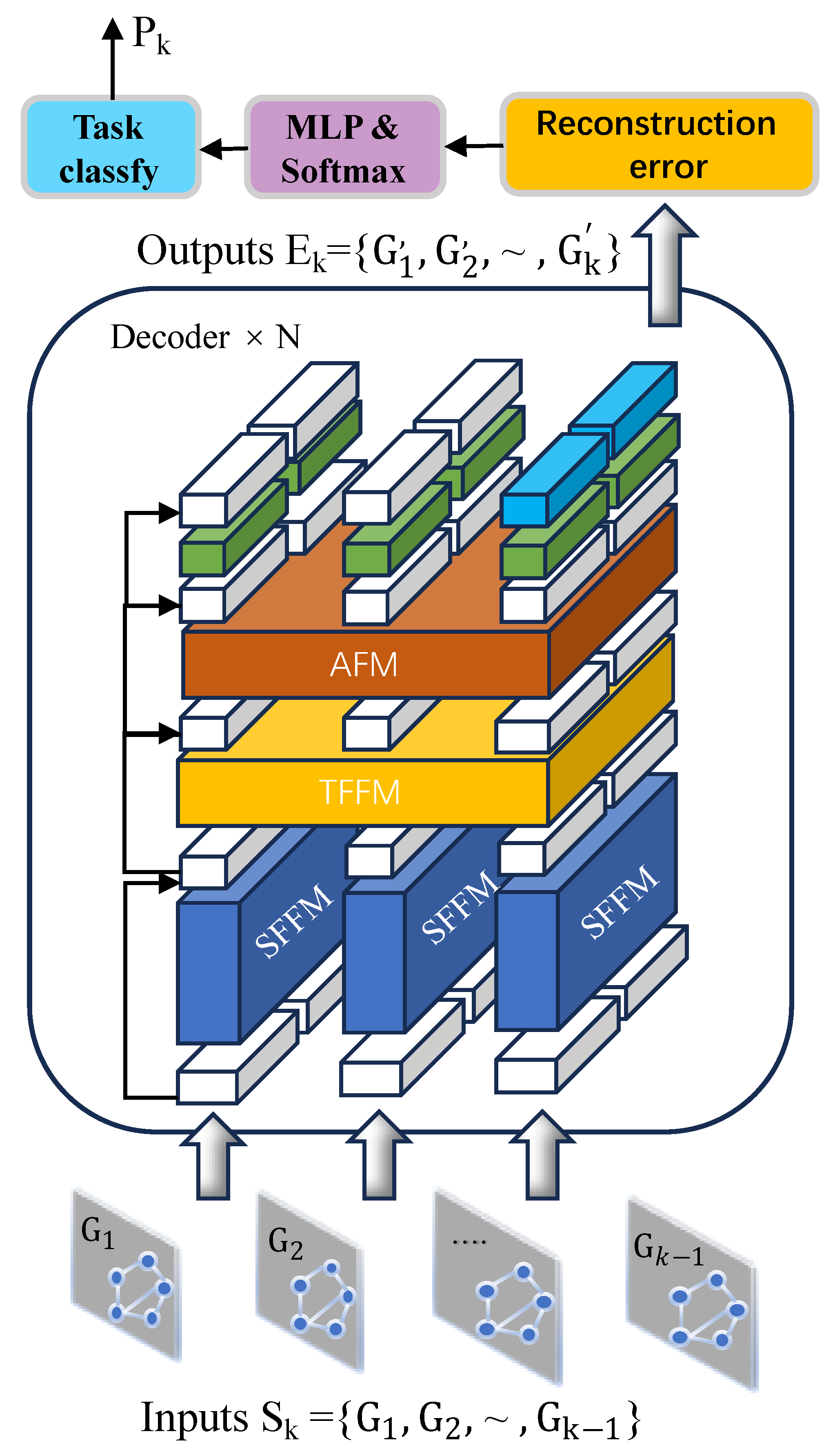
In this section, we provide a detailed description of the proposed method, GSTGPT. First, we project the raw multi-modal input data into a unified feature space through an embedding layer, ensuring that all three modalities share the same feature dimension [36]. Subsequently, we convert the input sequence S k into an initial representation I N 0 . In the decoder stage, we primarily employ a Temporal Feature Fusion Module (TFFM) and a Spatial Feature Fusion Module (SFFM) to iteratively update the input sequence S k , which consists of K graphs, while modeling the interdependencies among multi-modal data. Additionally, we propose an Attention-Enhancing Fusion Module (AFM), which enhances the model’s capacity for information representation by concatenating the original input features with the output from a multi-head attention mechanism. The operation of each decoder layer can be formally defined as follows:
I N 1 = Norm ( I N 0 + SFFM ( I N 0 ) ) , I N 2 = Norm ( I N 1 + Mask ( TFFM ( I N 1 ) ) ) , I N 3 = Norm ( I N 2 + Dropout ( AFM ( I N 2 ) ) ) , E K = Norm ( I N 3 + MLP ( I N 3 ) ) ,
Subsequently, we pre-train GSTGPT on the first k 1 normal sequences G k , enabling the model to learn the underlying patterns and structures of normal system behavior. After pre-training, GSTGPT can generate the next sequence G k at the subsequent time step based on a given portion of the sequence.
Inspired by LogGPT and LogPrompt, during the fine-tuning phase, we define a set of prompts P = { G 1 : t i } i = 1 K , where G 1 : t i G 1 : K i and G 1 : K i S k . These prompts are fed into the pre-trained GSTGPT model as the starting point for generating subsequent sequences. The model incrementally generates the subsequent sequence G k based on the given prompt G 1 : t i . Finally, anomaly classification is achieved by constructing the error between multi-source data, with the overall process illustrated in Figure 3.

4.1. GPT with Spatial Feature Fusion Module

Similar to the Graph Attention Network [37], the Spatial Feature Fusion Module (SFFM) updates node and edge features by aggregating information from neighboring nodes or edges. The objective is to update the input feature graph G k = V k , E k , M k by refining the representations of all existing nodes and edges.
Taking node update as an example, each node’s features are updated by aggregating information from its adjacent edges. Here, N i denotes a node in the graph, which corresponds to a microservice instance, and the edges represent actual invocation relationships between service instances. The attention score α i j , enclosed in parentheses, quantifies the importance of node j to node i, and is computed using a multi-head attention mechanism as follows:
α i j = LeakyReLU a W h i W h j e i j ,
Here, α i j denotes the attention score from node i to node j, which measures the importance of node j when updating the representation of node i. The operator represents the concatenation of vectors. Specifically, h i and h j are the input feature vectors of the source and target nodes, respectively, and  e i j is the feature vector associated with the edge connecting node i to node j.
During the node update process, we utilize a mapping matrix to determine the actual connectivity between nodes and edges. For each node, the attention contributions from all its adjacent edges are aggregated, effectively enabling a feature injection from edges to nodes. This mechanism ensures that each updated node representation incorporates not only its original metric and log features, but also the trace-related interaction features from neighboring edges. For example, consider node N 0 , which has two adjacent edges: Edge0 and Edge3. If their respective attention contributions to N 0 are 0.2 and 0.7, the total attention score received by N 0 is 0.9. This edge-to-node information injection process is illustrated in Figure 4. At each time step k, the node representations corresponding to microservice instances are updated using multi-head attention as follows:
V k = MultiHead ( V k , V k , E k ) ,
Specifically, each attention head adopts a unique temporal attention mechanism, which can be formulated as:
SpatialFusion ( Q , K , V ) = Softmax Q K d k V ,
Finally, we update each head H i through the SFFM as H i = SporalFusion ( V k , V k , E k ) .

4.2. GPT with Temporal Feature Fusion Module

In microservice systems, different modal features exhibit clear temporal characteristics. To model both intra-modal and inter-modal temporal dependencies, we propose a Temporal Feature Fusion Module (TFFM). This module employs an extended multi-head attention mechanism to capture the autocorrelated information along the temporal dimension.
First, we compute the average attention score C across multiple modalities based on the three new feature sequences obtained from the Spatial Feature Fusion Module (SFFM). Then, we apply an extended multi-head attention mechanism to model the inter-modal correlations for each modality at time step t. Consequently, the Temporal Feature Fusion Module (TFFM) captures the temporal dependencies among data points within the sliding window S K . The overall process is illustrated in Figure 5. Taking the log feature as an example, the temporal dependency of the log feature sequence can be formulated as follows:
L 1 : k = Multihead ( L 1 : k , L 1 : k , L 1 : k , C ) ,
In TFFM, we represent each head H i as:
H i = TemporalFusion ( L 1 : i W i Q , L 1 : i W i K , L 1 : i W i V ) ,
where W i is the corresponding weight matrix.
For the metric and trace features, we apply the same updating process using TFFM as we did for the log features, resulting in M 1 : K and T 1 : K , respectively. Finally, within the continuous sliding window S k , we establish global temporal correlations across all modalities. The update process for the entire sliding window S k can be expressed by the following formula:
S k = TFFM Norm S k + S k SFFM .

4.3. Attention-Enhancing Fusion Module

After processing with the SFFM and TFFM modules, we can establish useful interrelationships among multiple graphs in the sliding window S k , while maintaining temporal dependencies at time point t. Next, we specifically designed an Attention-Enhanced Feature Fusion (AMF) module, aimed at processing multi-modal and multi-dimensional sequence feature data. The core idea of the AMF module is to implement interaction and fusion between different modalities through a refined attention mechanism, thereby enhancing the model’s ability to capture key information.
First, for a specific time point t, we use the multi-head self-attention mechanism to independently enhance the features [38] of the three modalities: nodes, edges, and logs. This attention mechanism enables the model to dynamically focus on different feature subspaces within each modality, allowing the model to automatically identify and emphasize key features that contribute to improving classification or prediction performance.
For each modality, we use the multi-head self-attention mechanism to focus on key features. Taking log features as an example, the input log features are mapped into query, key, and value matrices:
Q log = W Q F Log + b Q , K log = W K F Log + b K , V log = W V F Log + b V
The symbol ∗ represents the multiplication operation, W is the weight matrix, and  b Q , b K , and  b V are the bias terms, which help the model better fit the data. The entire process is represented by the following formula:
F log - enhanced = ReLU Softmax Q K T d V + O
where O is a learnable parameter, the bias term, which helps the model better fit the data.
In this process, after applying multi-head attention, we further enhance the feature representation of F log through residual connections and nonlinear activation to obtain the enhanced feature representation F log - enhanced . Using the same approach, we apply feature enhancement to the three modalities F log , F metrics , and  F trace , resulting in F log - enhanced , F metrics - enhanced , and  F trace - enhanced , respectively. It is worth noting that in the AMF module, we generate the final multimodal representation by performing weighted cross-modal fusion on the attention-enhanced features. The update operation for cross-modal feature fusion can be expressed by the following formula:
F log - fused = a F log - enhanced + b F metric - enhanced + c F trace - enhanced
where a, b, and c are learnable weights that are learned through training.
We leverage the self-attention mechanism of the Adaptive Fusion Module to enhance the feature space, effectively capturing the complex latent patterns within individual modal features. This enhancement further improves the model’s representation capability. Ultimately, the features from all modalities are dynamically weighted and fused, followed by classification to generate the final output. In summary, the incorporation of AFM enables the model to focus more effectively on critical modal features, thereby boosting its representational power. This process can be formulated within the sliding window S K as follows:
S K AFM = AFM Norm ( S K + S K SFFM )

4.4. Reconstruction Error

We perform anomaly detection by reconstructing the final predicted graph and the actual state graph to check whether service instances are anomalous. Therefore, this study employs a novel multimodal reconstruction error computation method based on learnable weighted fusion. Traditional reconstruction error computation typically uses a single loss function, which does not fully consider the heterogeneity and relative importance of multimodal data, often leading to a decrease in overall model performance. To address this issue, this study designs a new reconstruction error computation framework to calculate the distance between the reconstructed and actual values, denoted as R E k , as described below:
R E k = G k G k 2 2 , P k = Softmax MLP G k G k
Specifically, we choose the Huber loss function to calculate the reconstruction error for different modal data. The Huber loss function is defined such that when the difference is smaller than a threshold, the squared error is used; when the difference exceeds the threshold, a linear penalty is applied. We pass each modality of data through an embedding layer and the model reconstruction to obtain the reconstruction results [12]. The Huber loss for each modality is then computed to obtain its respective reconstruction error. The specific process is shown in Algorithm 1. The Huber loss calculation process is as follows:
L Huber ( X , Y ) = 1 2 ( X f Y f ) 2 , if | X f Y f |   δ   δ · | X f Y f | 1 2 δ , otherwise
Next, we obtain the reconstruction errors for the three modalities: L log , L metrics , and  L trace . Due to the differences in feature dimensions across modalities, this study introduces a linear projection layer to unify the feature dimensions, ensuring that the errors of each modality can be fused in a common space. Meanwhile, to further improve the effectiveness of multimodal fusion, this study designs a learnable fusion weight that allows the model to automatically optimize the importance of different modality data, dynamically adjusting the contribution of each modality during training. Then, we apply the softmax function to normalize the weights, thereby enhancing anomaly detection performance. The final multimodal fusion reconstruction error is defined as the sum of the products of each modality’s reconstruction error and its corresponding weight:
L recon k = α · L log k + β · L metrics k + γ · L trace k
In practical applications, the model makes anomaly detection decisions based on the fused reconstruction error. Typically, the reconstruction error of normal data is lower, while that of anomalous data is higher. Based on this characteristic, a threshold can be set to effectively identify anomalous data. The reconstruction error computation method optimized above can improve the model’s stability and robustness, solving the modality imbalance problem present in traditional methods, and effectively enhancing the overall performance of anomaly detection in microservice systems.
Algorithm 1 The GSTGPT training algorithm
  • Require: Sliding window for training { S k } k = 1 T , Decoder D, Iteration limit N.
  •  1: Initialize weights E, D
  •  2: i 1
  •  3: while  i < N   do
  •  4:    for  k = 1  to T do
  •  5:         E k InputEmbedding ( S k )
  •  6:         E k E ( E k )
  •  7:         G k D ( E k , E k )
  •  8:        if  G k G k < δ  then
  •  9:              L 1 2 G k G k 2
  • 10:        else
  • 11:            L δ · G k G k 1 2 δ
  • 12:        end if
  • 13:    end for
  • 14:    Update the weights of E, D using L
  • 15:     i i + 1
  • 16: end while

5. Experiments

5.1. Datasets

Micro-Service Dataset for Anomaly Detection(MSDS): MSDS [16] is an important benchmark dataset in the field of multivariate time series anomaly detection, widely used in intelligent operation and maintenance research for servers and cloud computing systems. This dataset simulates the multidimensional performance monitoring metrics of production-grade servers in real-world operating environments, including CPU usage, memory usage, disk read/write rates, network bandwidth, and more. Each metric is continuously sampled at fixed time intervals (e.g., once per minute), forming high-dimensional time series data.
AIOps-Challenge: The AIOps-Challenge [32] is a benchmark dataset used in recent years to evaluate the capabilities of artificial intelligence in operations (AIOps), particularly in anomaly detection and root cause analysis tasks. This dataset simulates typical operational scenarios in distributed microservices systems and covers various data types, including logs, metrics, and traces, supporting multi-source data joint modeling.

5.2. Baselines

In the experiments, we compare and test GSTGPT against several benchmark models, including deep learning models and the language model GPT.
TraceAnomaly: This method [25] constructs system and software traces into a call graph and learns joint features of service call structures and behaviors through a graph neural network, providing an online detection method for anomaly detection at the microservice.
TranAD: This model is a Transformer-based detection method that uses the Transformer to capture temporal dependencies. It jointly models normal behavior patterns through reconstruction and adversarial mechanisms, achieving efficient and robust time-series anomaly detection in unsupervised scenarios.
SCWarn: SCWarn [39] is based on dynamic service call graphs and uses a time-aware graph neural network to model structural dependencies and behavioral evolution between services. It efficiently captures the propagation of anomalies across microservice chains and enables fine-grained service anomaly detection.
PLELog: PLELog utilizes a pre-trained language model to perform deep semantic modeling on unstructured logs and combines contextual windows to enhance anomaly recognition. It is a log anomaly detection method that requires no templates, is highly transferable, and excels in semantic understanding.
LogGPT: LogGPT is a log anomaly detection method based on an autoregressive language model. It learns the generation patterns of log sequences and identifies anomalous events in the log flow by utilizing prediction errors.

5.3. Experiment Settings

For some benchmark models that only require log data, such as LogGPT, we first use Drain to parse raw log messages into log keys. Using the parsed log keys, we construct the vocabulary required for the LogGPT model to detect anomalies. The first 90% of the data is used for training, and the remaining 10% is used for validation. For models other than LogGPT, we use 60% of the data for training, 10% for validation, and the remaining 30% for testing. We evaluate the proposed method using the following five model evaluation metrics: Precision, Recall, F1-Score, Average Precision, and AUC. PR represents the proportion of true positives among all predicted events. RC represents the probability of the model detecting true samples among all labeled normal samples. F1-Score is the weighted average of Precision and Recall, balancing the importance of both. AP is the area under the Precision–Recall curve and can be viewed as the comprehensive performance of F1 at different thresholds. AUC represents the classification performance of the model, with higher AUC values indicating stronger overall classification ability.
Our experiments are conducted on a Windows-based workstation equipped with dual NVIDIA RTX 2080 Ti GPUs (22 GB total GPU memory), an Intel® Xeon® Platinum 8255C CPU with 9 cores per GPU, and 48 GB of RAM. The system is configured with 30 GB system disk and a 50 GB expandable data disk. Our implementation is developed using Python 3.8, PyTorch 1.12.0 with CUDA 11.7, and PyTorch Geometric 2.6.0. The model was trained for up to 300 epochs with a batch size of 32, window size of 10. GSTGPT is configured with 8 decoder layers, 6 self-attention heads, an embedding dimension of 60, a positional encoding dimension of 512, a feedforward layer of 240 dimensions, and a GELU activation function, with a total of approximately 500,000 parameters. We employed the AdaBelief optimizer with an initial learning rate of 0.001. For models like LogGPT, we use 90% of the data for training and the remaining 10% for validation. For other models, 60% of the data is used for training, 10% for validation, and 30% for testing.

5.4. Experimental Results

Performance on Anomaly Detection:
Firstly, from Table 1, it can be observed that TraceAnomaly achieved the best RC score on the MSDS dataset when handling the anomaly detection task for single-trace data, surpassing other benchmark models. However, in terms of detection accuracy (PR), TraceAnomaly performs worse than LogGPT and GSTGPT. This indicates that large language models have certain advantages when handling few-sample modal data, especially in improving accuracy.
PLELog and TranAD are essentially Transformer-based architectures designed for multimodal implementation. However, the results in Table 2 show that these methods still have limitations when the data comes from unknown datasets, performing worse than other models. SCWarn has certain advantages in multimodal fusion, but based on the results from our dataset, it falls short compared to other benchmark models. Furthermore, through comparative experiments, it can be observed that LogGPT performs excellently on the MSDS dataset, achieving a PR score of 0.978, surpassing other detection models. This demonstrates the unique advantages of large language models in log data anomaly detection. However, performance on the AIOps-Challenge dataset indicates that the model still faces difficulties in anomaly detection for specific datasets and in processing multimodal data.
Finally, we found that GSTGPT achieved the highest F1 scores of 0.957 and 0.967 on the MSDS and AIOps-Challenge datasets, respectively, after integrating multiple feature fusion methods. These overall high scores indicate that GSTGPT outperforms other benchmark models in anomaly detection tasks, showcasing its outstanding performance.

5.5. Ablation Studies

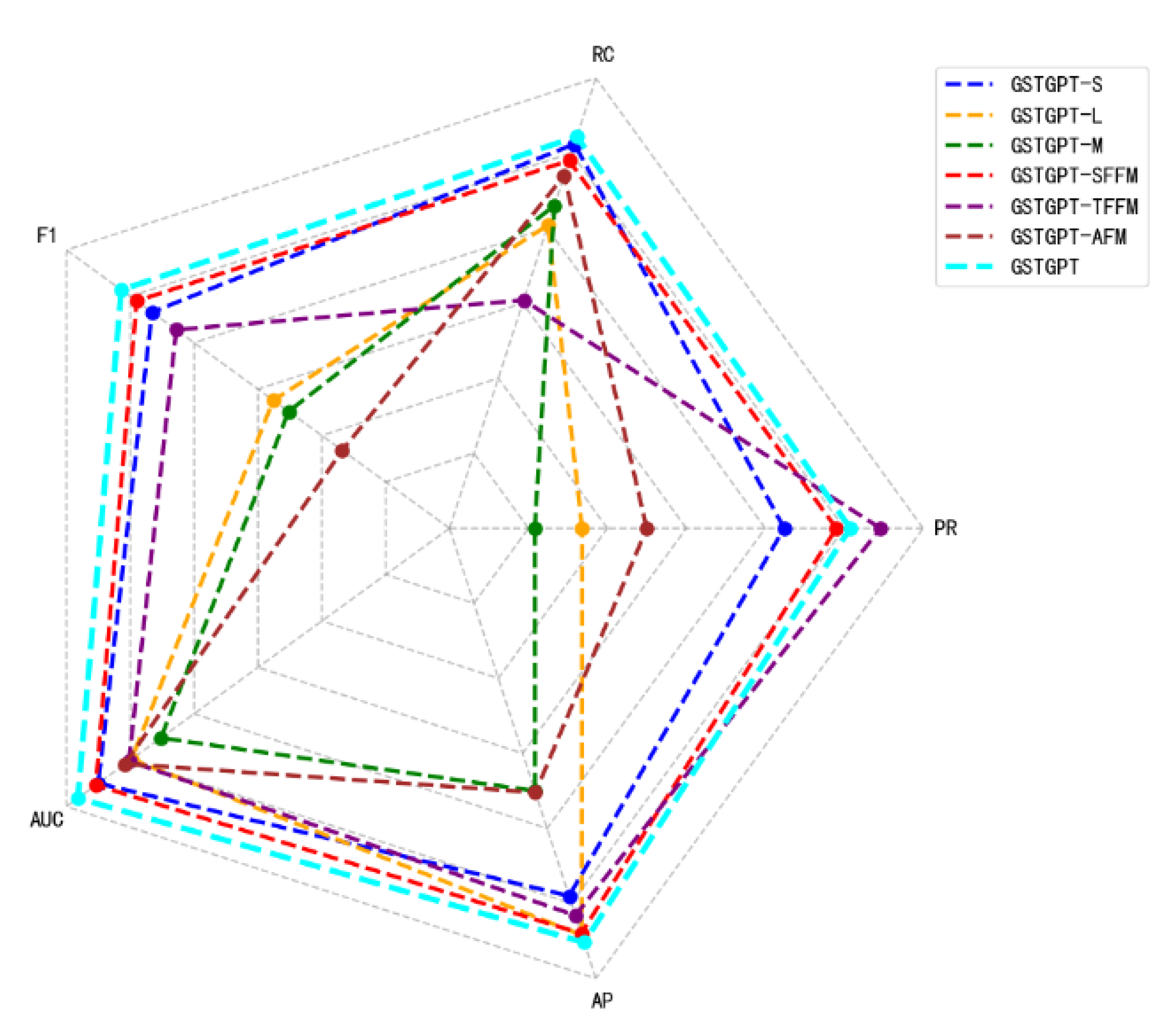
To investigate the practical contribution of the TFFM, SFFM, and the AFM to the overall performance of the proposed GSTGPT framework, we designed a set of ablation experiments to compare the impact of each individual component. In addition, we also examine the performance of the proposed method under limited modality settings, where only partial sources of data (e.g., logs or metrics alone) are available. To provide a more intuitive comparison, we also visualize the experimental outcomes using a radar Figure 6, which highlights the relative effectiveness of each module and configuration.
To thoroughly assess the impact of each individual module and modality on the performance of the proposed GSTGPT framework, we conducted a series of experiments by independently removing specific modules or data inputs. The results are presented in Table 3.
Specifically, we conducted separate ablation experiments on the three data modalities. The results of GSTGPT-S and GSTGPT-L indicate that constructing the graph solely based on a single modality is insufficient for comprehensive feature extraction. In the case of GSTGPT-M, where the system status information is excluded from the edge structure during graph construction, the model lacks edge-level features and can only utilize node features derived from logs and metrics. This limits the ability of the graph to effectively integrate features through structural relationships. Notably, GSTGPT-M yields the lowest performance among all ablation variants, achieving only an F1 score of 0.826. These results collectively confirm that GSTGPT benefits significantly from the fusion of heterogeneous modalities for effective anomaly detection. Moreover, as shown in Table 3, our approach outperforms the log-only language model LogGPT by a considerable margin. Specifically, GSTGPT achieves an average F1 score improvement of 9.55%, demonstrating the advantage of incorporating multi-modal data over relying solely on language modeling.
It is also worth noting that the full GSTGPT model outperforms its ablated variants, including GSTGPT-SFFM, GSTGPT-TFFM, and GSTGPT-AFM. This highlights the positive contribution of each of the proposed modules—namely, the SFFM, TFFM, and AFM to the overall performance of GSTGPT. In particular, as shown in Table 3, the F1 score of GSTGPT-SFFM is higher than all other variants except the complete GSTGPT model, indicating that the spatial attention module effectively captures spatial dependencies within the graph structure. Similarly, the experimental results for GSTGPT-TFFM demonstrate that the temporal attention module plays a key role in modeling complex temporal dependencies. Finally, the GSTGPT-AFM variant also shows performance gains, suggesting that the AFM helps the model focus on salient features within the temporal window, thereby improving anomaly detection precision.

Parameter Analysis

GSTGPT performs anomaly detection through classification based on reconstruction error, where the weight label_weight directly affects the overall model loss. Additionally, we note that the number of decoder layers and the training scale also influence the final experimental results. We set up experiments on the MSDS dataset to evaluate the choice of these hyperparameters.
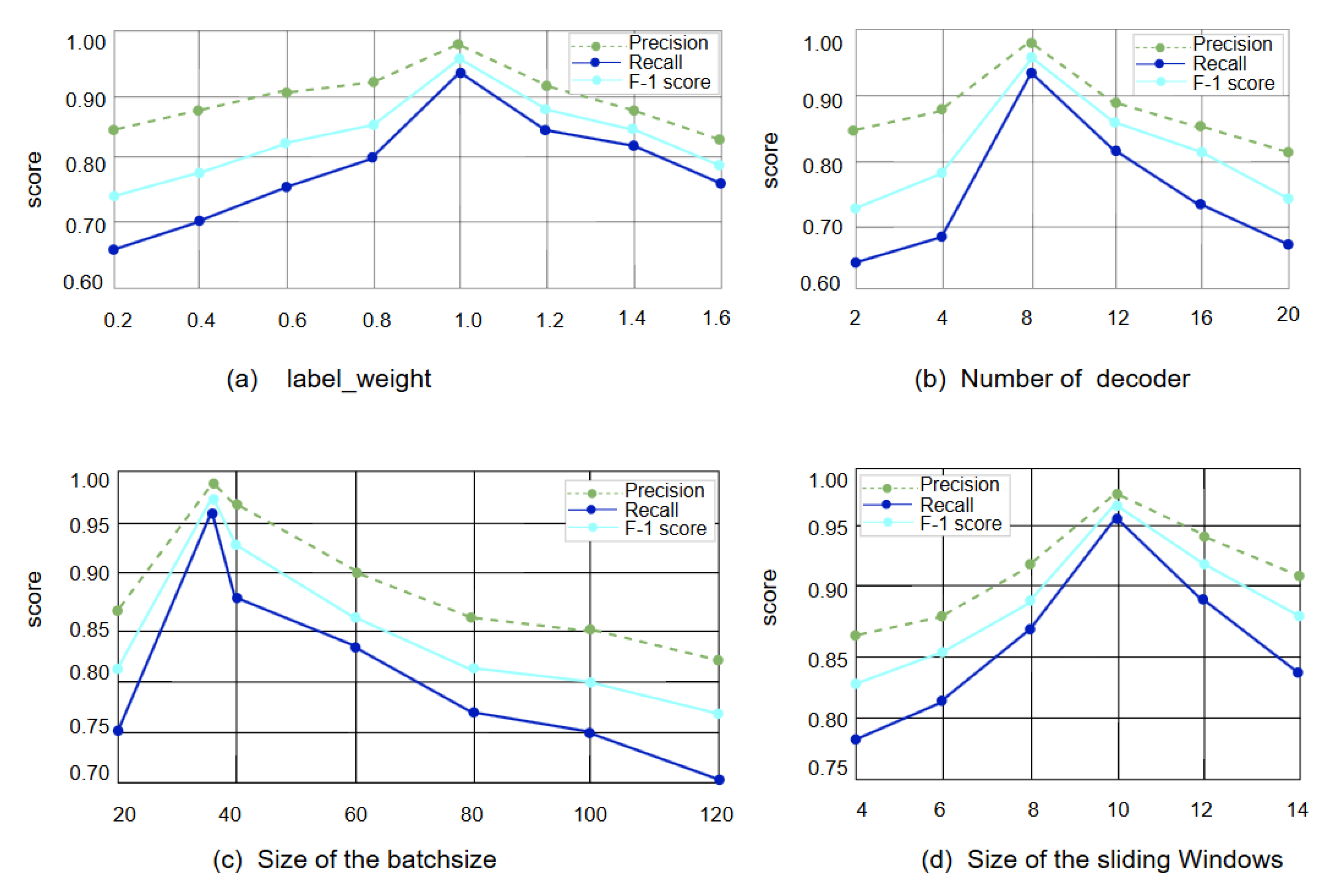
The impact of different weights label_weight on the model’s precision, recall, and F1 score is shown in Figure 7. It is clearly observed that when the weight label_weight is in the range of 0.4 to 1, as the weight increases, the F1 score continuously improves until it reaches its maximum. However, once the threshold of 1 is exceeded, the F1 score sharply decreases. The main reason for this phenomenon is that if the weight is greater than or less than the critical threshold of 1.0, it may either amplify or reduce the impact of these samples on the overall loss. The threshold of 1.0 allows the model to better balance the effects of normal, abnormal, and boundary samples during loss calculation.
The number of decoder layers directly determines the depth and complexity of the reconstruction process. We evaluated the impact of the number of decoder layers on the model’s precision, recall, and F1 score. As shown in Figure 7, when the number of decoder layers is small, the F1 score is low, mainly because the model cannot capture deep features and complex patterns. When the number of decoder layers increases to 20, the F1 score is far lower than when the number of layers is 8. This phenomenon may occur because each additional decoder layer significantly increases the number of parameters and computational complexity, which not only extends training time but may also require higher memory usage. The comparative experimental results show that selecting 8 decoder layers can better address this contradiction, and at this point, the model’s precision, recall, and F1 score reach their best performance.
The batch_size defines the number of samples input to the model for training or inference at a time. It not only affects the gradient calculation and parameter updates during the training process but also influences model stability. Figure 7 shows that a larger batch_size provides more stable gradient estimation and accelerates training convergence, but it also increases memory consumption. A smaller batch_size may make the gradient updates more noisy, leading to instability during training. Ultimately, we found that a batch_size of 32 contributed the most to the model’s performance.
The size of the sliding window directly affects the model’s ability to capture temporal dependencies and its accuracy in identifying anomalies. Through comparative experiments, we found that with a small window size, the model’s F1 score may be relatively low, possibly because the model cannot fully utilize long-term information in the time series. On the other hand, a large-scale window increases the model’s computational load and memory consumption, which may reduce the model’s real-time performance. Ultimately, we found that choosing a sliding window size of 10 best utilizes the information in the time series for anomaly detection.
Finally, we evaluate the runtime efficiency of GSTGPT by analyzing the time cost associated with each stage of multi-source data processing across two benchmark datasets. Additionally, we report the average number of observed metrics, logs, and traces within each sliding time window interval. The results are summarized in Table 4, where # Metrics, # Logs, and # Traces represent the average number of metric entries, log events, and trace spans, respectively, observed within each processing interval. Experimental results indicate that the time consumed for multi-source data preprocessing and graph construction is significantly lower than the system’s time interval between two consecutive observations. This demonstrates that our proposed model is well-suited for real-time anomaly detection applications with high efficiency.

6. Conclusions

We propose an anomaly detection model based on the GPT architecture, GSTGPT, which leverages a decoder-based architecture to effectively integrate multi-source time series data for anomaly detection. GSTGPT utilizes the Temporal Attention Module and Spatial Attention Module to keenly capture the complex underlying relationships embedded in the sequences. Subsequently, GSTGPT enhances knowledge and feature extraction through the Attention Enhancement Module, improving its ability to model complex data relationships. Finally, we compare the model’s prediction of the final system state to achieve anomaly detection. Compared to the best baseline methods, our proposed approach achieves F1 scores of 0.957 and 0.967 on two real-world datasets after fusing various features, resulting in improvements of 1.5% and 8.3%, respectively.
For future work, we suggest extending this method to the GPT-3.5 or GPT-4.0 architecture via API or other methods to further improve prediction accuracy.

Author Contributions

Conceptualization, J.L. (Jizhao Liu) and M.F.; methodology, S.Z.; validation, F.S.; formal analysis, J.L. (Jun Li); writing—original draft, J.L. (Jizhao Liu); writing—review and editing, M.F.; supervision, F.S. and J.L. (Jun Li); project administration, S.Z.; funding acquisition, J.L. (Jizhao Liu) and M.F. All authors have read and agreed to the published version of the manuscript.

Funding

This work was supported in part by the Key Backbone Teachers Support Program of Zhongyuan University of Technology under Project GG202417, and in part by the Key Research and Development Program of Henan under Grant 251111212000.

Institutional Review Board Statement

Not applicable.

Informed Consent Statement

Not applicable.

Data Availability Statement

The original contributions presented in this study are included in this article. Further inquiries can be directed to the corresponding authors.

Acknowledgments

The authors have reviewed and edited the output and take full responsibility for the content of this publication. The authors sincerely thank the editors and reviewers for their professional insights, which have greatly improved the technical depth and communicative clarity of this article.

Conflicts of Interest

The authors declare that there are no conflicts of interest.

References

  1. Hariri, S.; Kind, M.C.; Brunner, R.J. Extended isolation forest. IEEE Trans. Knowl. Data Eng. 2019, 33, 1479–1489. [Google Scholar] [CrossRef]
  2. Hejazi, M.; Singh, Y.P. One-class support vector machines approach to anomaly detection. Appl. Artif. Intell. 2013, 27, 351–366. [Google Scholar] [CrossRef]
  3. Nanduri, A.; Sherry, L. Anomaly detection in aircraft data using Recurrent Neural Net-works (RNN). In Proceedings of the 2016 Integrated Communications Navigation and Surveillance (ICNS), Herndon, VA, USA, 19–21 April 2016; p. 5C2–1. [Google Scholar]
  4. Laghrissi, F.; Douzi, S.; Douzi, K.; Hssina, B. Intrusion detection systems using long short-term memory (LSTM). J. Big Data 2021, 8, 65. [Google Scholar] [CrossRef]
  5. Xu, W.; Jang-Jaccard, J.; Singh, A.; Wei, Y.; Sabrina, F. Improving performance of autoencoder-based net-work anomaly detection on nsl-kdd dataset. IEEE Access 2021, 9, 140136–140146. [Google Scholar] [CrossRef]
  6. Sabuhi, M.; Zhou, M.; Bezemer, C.P.; Musilek, P. Applications of generative adversarial networks in anomaly detection: A systematic literature review. IEEE Access 2021, 9, 161003–161029. [Google Scholar] [CrossRef]
  7. Guo, H.; Yuan, S.; Wu, X. Logbert: Log anomaly detection via bert. In Proceedings of the 2021 International Joint Conference on Neural Networks (IJCNN), Shenzhen, China, 18–22 July 2021; pp. 1–8. [Google Scholar]
  8. Zhang, X.; Xu, Y.; Lin, Q.; Qiao, B.; Zhang, H.; Dang, Y.; Xie, C.; Yang, X.; Cheng, Q.; Li, Z.; et al. Robust log-based anomaly detection on unstable log data. In Proceedings of the 2019 27th ACM Joint Meeting on European Software Engineering Conference and Symposium on the Foundations of Software Engineering, Tallinn, Estonia, 26–30 August 2019; pp. 807–817. [Google Scholar]
  9. Lu, S.; Wei, X.; Li, Y.; Wang, L. Detecting anomaly in big data system logs using convolu-tional neural network. In Proceedings of the 2018 IEEE 16th Intl Conf on Dependable, Autonomic and Secure Computing, 16th Intl Conf on Pervasive Intelligence and Computing, 4th Intl Conf on Big Data Intelligence and Computing and Cyber Science and Technology Congress (DASC/PiCom/DataCom/CyberSciTech), Athens, Greece, 12–15 August 2018; pp. 151–158. [Google Scholar]
  10. Yang, L.; Chen, J.; Wang, Z.; Wang, W.; Jiang, J.; Dong, X.; Zhang, W. Semi-supervised log-based anomaly detection via probabilistic label estimation. In Proceedings of the 2021 IEEE/ACM 43rd International Conference on Software Engineering (ICSE), Madrid, Spain, 22–30 May 2021; pp. 1448–1460. [Google Scholar]
  11. Tuli, S.; Casale, G.; Jennings, N.R. Tranad: Deep transformer networks for anomaly detection in multivariate time series data. arXiv 2022, arXiv:2201.07284. [Google Scholar] [CrossRef]
  12. Zhao, N.; Chen, J.; Yu, Z.; Wang, H.; Li, J.; Qiu, B.; Xu, H.; Zhang, W.; Sui, K.; Pei, D. Identifying bad software changes via multimodal anomaly detection for online service systems. In Proceedings of the 29th ACM Joint Meeting on European Software Engineering Conference and Symposium on the Foundations of Software Engineering, Athens, Greece, 23–28 August 2021; pp. 527–539. [Google Scholar]
  13. Lee, C.; Yang, T.; Chen, Z.; Su, Y.; Lyu, M.R. Eadro: An end-to-end troubleshooting frame-work for microservices on multi-source data. In Proceedings of the 2023 IEEE/ACM 45th International Conference on Software Engineering (ICSE), Melbourne, Australia, 14–20 May 2023; pp. 1750–1762. [Google Scholar]
  14. Zhao, C.; Ma, M.; Zhong, Z.; Zhang, S.; Tan, Z.; Xiong, X.; Yu, L.; Feng, J.; Sun, Y.; Zhang, Y.; et al. Robust multimodal failure detection for microservice systems. In Proceedings of the 29th ACM SIGKDD Conference on Knowledge Discovery and Data Mining, Long Beach, CA, USA, 6–10 August 2023; pp. 5639–5649. [Google Scholar]
  15. Zhang, S.; Jin, P.; Lin, Z.; Sun, Y.; Zhang, B.; Xia, S.; Li, Z.; Zhong, Z.; Ma, M.; Jin, W.; et al. Robust failure diagnosis of microservice system through multimodal data. IEEE Trans. Serv. Comput. 2023, 16, 3851–3864. [Google Scholar] [CrossRef]
  16. Nedelkoski, S.; Bogatinovski, J.; Mandapati, A.K.; Becker, S.; Cardoso, J.; Kao, O. Multi-source distributed system data for ai-powered analytics. In Proceedings of the European Conference on Service-Oriented and Cloud Computing, Heraklion, Greece, 28–30 September 2020; Springer International Publishing: Cham, Switzerland, 2020; pp. 161–176. [Google Scholar]
  17. Liu, Y.; Tao, S.; Meng, W.; Yao, F.; Zhao, X.; Yang, H. Logprompt: Prompt engineering to-wards zero-shot and interpretable log analysis. In Proceedings of the 2024 IEEE/ACM 46th International Conference on Software Engineering: Companion Proceedings, Lisbon, Portugal, 14–20 April 2024; pp. 364–365. [Google Scholar]
  18. Han, X.; Yuan, S.; Trabelsi, M. Loggpt: Log anomaly detection via gpt. In Proceedings of the 2023 IEEE International Conference on Big Data (BigData), Sorrento, Italy, 15–18 December 2023; pp. 1117–1122. [Google Scholar]
  19. Xu, W.; Huang, L.; Fox, A.; Patterson, D.; Jordan, M.I. Detecting large-scale system prob-lems by mining console logs. In Proceedings of the ACM SIGOPS 22nd Symposium on Operating Systems Principles, Big Sky, MT, USA, 11–14 October 2009; pp. 117–132. [Google Scholar]
  20. Vaswani, A.; Shazeer, N.; Parmar, N.; Uszkoreit, J.; Jones, L.; Gomez, A.N.; Kaiser, L.; Polosukhin, I. Attention is all you need. Adv. Neural Inf. Process. Syst. 2017, 30, 5998–6008. [Google Scholar]
  21. Kurita, T. Principal component analysis (PCA). In Computer Vision: A Reference Guide; Springer International Publishing: Cham, Switzerland, 2021; pp. 1013–1016. [Google Scholar]
  22. Almodovar, C.; Sabrina, F.; Karimi, S.; Azad, S. LogFiT: Log anomaly detection using fine-tuned language models. IEEE Trans. Netw. Serv. Manag. 2024, 21, 1715–1723. [Google Scholar] [CrossRef]
  23. Du, M.; Li, F.; Zheng, G.; Srikumar, V. Deeplog: Anomaly detection and diagnosis from system logs through deep learning. In Proceedings of the 2017 ACM SIGSAC Conference on Computer and Communications Security, Dallas, TX, USA, 30 October–3 November 2017; pp. 1285–1298. [Google Scholar]
  24. Meng, W.; Liu, Y.; Zhu, Y.; Zhang, S.; Pei, D.; Liu, Y.; Chen, Y.; Zhang, R.; Tao, S.; Sun, P.; et al. Loganomaly: Unsuper-vised detection of sequential and quantitative anomalies in unstructured logs. Int. Jt. Conf. Artif. Intell. 2019, 19, 4739–4745. [Google Scholar]
  25. Liu, P.; Xu, H.; Ouyang, Q.; Jiao, R.; Chen, Z.; Zhang, S.; Yang, J.; Mo, L.; Zeng, J.; Xue, W.; et al. Unsupervised detection of microservice trace anomalies through service-level deep bayesian networks. In Proceedings of the 2020 IEEE 31st International Symposium on Software Reliability Engineering (ISSRE), Coimbra, Portugal, 12–15 October 2020; pp. 48–58. [Google Scholar]
  26. Yang, Z.; Harris, I.G. LogLLaMA: Transformer-based log anomaly detection with LLaMA. arXiv 2025, arXiv:2503.14849. [Google Scholar]
  27. Gruver, N.; Finzi, M.; Qiu, S.; Wilson, A.G. Large language models are zero-shot time series forecasters. Adv. Neural Inf. Process. Syst. 2023, 36, 19622–19635. [Google Scholar]
  28. Zhou, T.; Niu, P.; Sun, L.; Jin, R. One fits all: Power general time series analysis by pretrained lm. Adv. Neural Inf. Process. Syst. 2023, 36, 43322–43355. [Google Scholar]
  29. Shi, X.; Xue, S.; Wang, K.; Zhou, F.; Zhang, J.; Zhou, J.; Tan, C.; Mei, H. Language models can improve event pre-diction by few-shot abductive reasoning. Adv. Neural Inf. Process. Syst. 2023, 36, 29532–29557. [Google Scholar]
  30. Liu, P.; Yuan, W.; Fu, J.; Jiang, Z.; Hayashi, H.; Neubig, G. Pre-train, prompt, and predict: A system-atic survey of prompting methods in natural language processing. ACM Comput. Surv. 2023, 55, 1–35. [Google Scholar] [CrossRef]
  31. Guan, W.; Cao, J.; Qian, S.; Gao, J.; Ouyang, C. Logllm: Log-based anomaly detection using large language models. arXiv 2024, arXiv:2411.08561. [Google Scholar]
  32. Li, Z.; Zhao, N.; Zhang, S.; Sun, Y.; Chen, P.; Wen, X.; Ma, M.; Pei, D. Constructing large-scale real-world benchmark datasets for aiops. arXiv 2022, arXiv:2208.03938. [Google Scholar]
  33. He, P.; Zhu, J.; Zheng, Z.; Lyu, M.R. Drain: An online log parsing approach with fixed depth tree. In Proceedings of the 2017 IEEE International Conference on Web Services (ICWS), Honolulu, HI, USA, 25–30 June 2017; pp. 33–40. [Google Scholar]
  34. Wang, Z.; Wu, Z.; Li, X.; Shao, H.; Han, T.; Xie, M. Attention-aware temporal–spatial graph neural net-work with multi-sensor information fusion for fault diagnosis. Knowl. Based Syst. 2023, 278, 110891. [Google Scholar] [CrossRef]
  35. Huang, J.; Yang, Y.; Yu, H.; Li, J.; Zheng, X. Twin graph-based anomaly detection via attentive multi-modal learning for microservice system. In Proceedings of the 2023 38th IEEE/ACM International Conference on Automated Software Engineering (ASE), Luxembourg, 11–15 September 2023; pp. 66–78. [Google Scholar]
  36. Liu, Y.; Li, Z.; Pan, S.; Gong, C.; Zhou, C.; Karypis, G. Anomaly detection on attributed networks via con-trastive self-supervised learning. IEEE Trans. Neural Netw. Learn. Syst. 2021, 33, 2378–2392. [Google Scholar] [CrossRef]
  37. Zhao, H.; Wang, Y.; Duan, J.; Huang, C.; Cao, D.; Tong, Y.; Xu, B.; Bai, J.; Tong, J.; Zhang, Q. Multivariate time-series anomaly detection via graph attention network. In Proceedings of the 2020 IEEE International Conference on Data Mining (ICDM), Sorrento, Italy, 17–20 November 2020; pp. 841–850. [Google Scholar]
  38. Xie, X.; Cui, Y.; Tan, T.; Zheng, X.; Yu, Z. Fusionmamba: Dynamic feature enhancement for multimodal image fusion with mamba. Vis. Intell. 2024, 2, 37. [Google Scholar] [CrossRef]
  39. Chen, Q.; Huang, G.; Wang, Y. The weighted cross-modal attention mechanism with sentiment prediction auxiliary task for multimodal sentiment analysis. IEEE/ACM Trans. Audio Speech Lang. Process. 2022, 30, 2689–2695. [Google Scholar] [CrossRef]
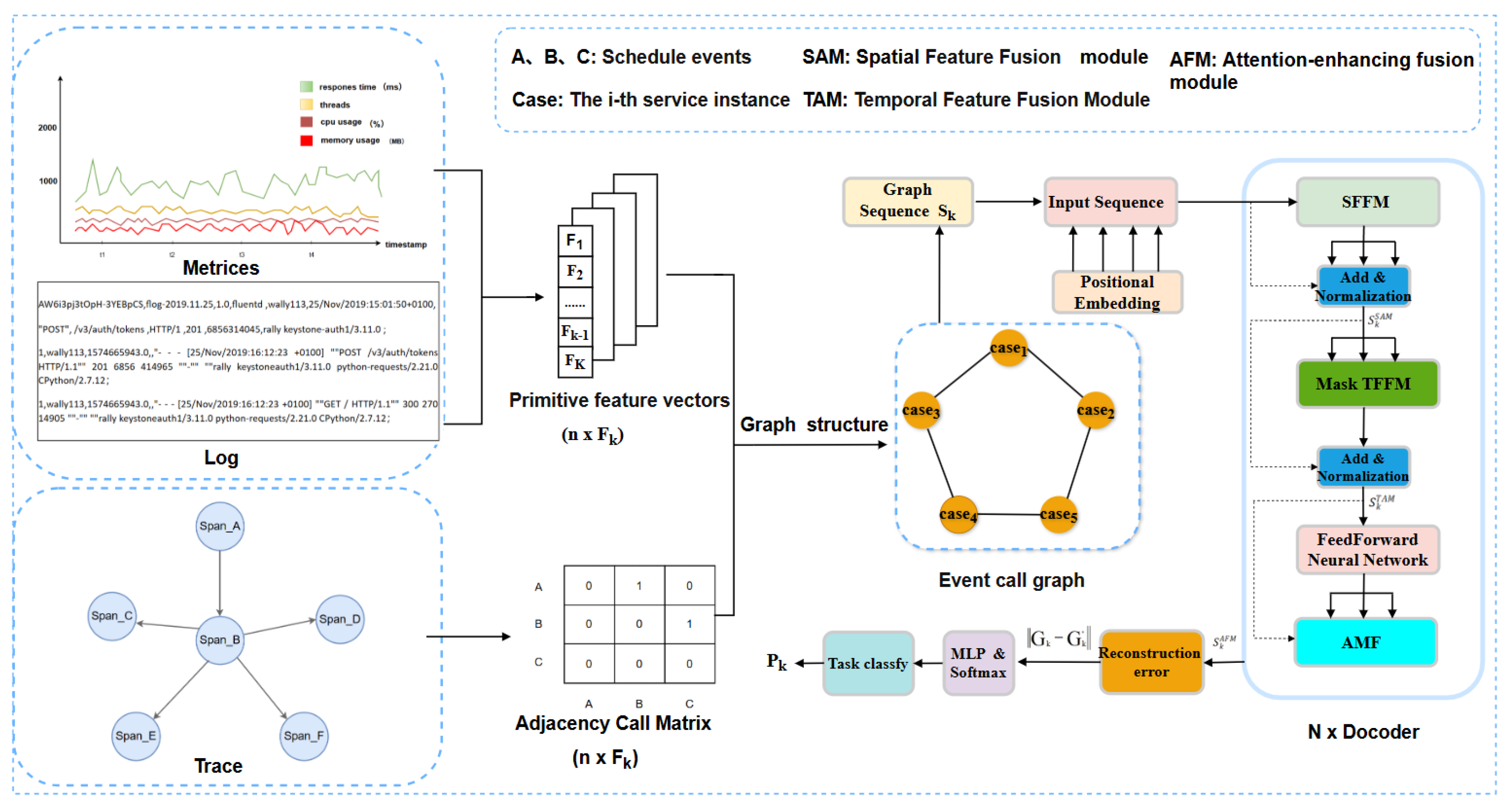
Figure 1. The overall architecture of the proposed GSTGPT model.
Information 16 00959 g001
Figure 2. Log keys are extracted from the MSDS dataset messages using a log parser. Messages with red underlines indicate the types of detailed system information captured by the corresponding log templates. ‘*’ indicates an abbreviated representation of the corresponding field in the template.
Information 16 00959 g002
Figure 3. The framework of GSTGPT.
Information 16 00959 g003
Figure 4. Update the features of nodes in the graph.
Information 16 00959 g004
Figure 5. Framework of GPT With Temporal Feature Fusion Module.
Information 16 00959 g005
Figure 6. Radar chart representation of ablation experiment results.
Information 16 00959 g006
Figure 7. The different F1 scores, Precision, and Recall scores for varying parameters.
Information 16 00959 g007
Table 1. Comparative experimental results on msds dataset and its baseline models (the bold black numbers in the table represent the best experimental results of a performance in the experiment).
MethodData UsedRCPRF1Baseline
TraceAnomalyTrace0.9890.9090.947GCN
TranADMetric0.7540.8140.782Transformer & GAN
SCWarnMetric & Log0.4400.3540.392DyGAT
PLELogLog0.6640.7240.692BERT
LogGPTLog0.9100.9780.943GPT
GSTGPTMetric & Log & Trace0.9610.9530.957GPT & GAT
Table 2. Comparative experimental results on aiops-challenge dataset and its baseline models.
MethodData UsedRCPRF1Baseline
TraceAnomalyTrace0.2460.8500.373GCN
TranADMetric0.8120.6540.724Transformer & GAN
SCWarnMetric & Log0.6450.8650.738DyGAT
PLELogLog0.2180.7520.338BERT
LogGPTLog0.9130.8750.893GPT
GSTGPTMetric & Log & Trace0.9640.9720.967GPT & GAT
Table 3. Ablation study results and performance on MSDS dataset.
MethodPRRCAPAUCF1
GSTGPT-S0.9120.9560.9450.9750.933
GSTGPT-L0.7840.9020.9710.9490.838
GSTGPT-M0.7540.9150.8750.9260.826
GSTGPT-SFFM0.9450.9450.9700.9770.945
GSTGPT-TFFM0.9730.8520.9580.9510.914
GSTGPT-AFM0.8250.9350.8760.9540.784
GSTGPT0.9530.9610.9760.9910.957
Table 4. Detailed data characteristics of the experimental dataset, as well as the processing time for a single sliding window and the entire dataset.
DatasetInterval time# Logs# Traces# instance*metric
MSDS3 s174167*4
AIOps45 s6012826540*25
DatasetTotal DurationTotal number of logsTotal number of TracesTotal number of metric
MSDS9965 s11,59512,18311,158
AIOps20,115 s75,52886,92472,247
DatasetPreprocessingConstructing graphDetectingTotal
MSDS0.027 s0.0012 s0.032 s0.0263 s
AIOps5.2554 s0.191 s0.248 s7.4324 s
Disclaimer/Publisher’s Note: The statements, opinions and data contained in all publications are solely those of the individual author(s) and contributor(s) and not of MDPI and/or the editor(s). MDPI and/or the editor(s) disclaim responsibility for any injury to people or property resulting from any ideas, methods, instructions or products referred to in the content.