Autoencoder-Based Poisoning Attack Detection in Graph Recommender Systems

Abstract

Graph-based Recommender Systems (GRSs) model complex user–item relationships. They offer improved accuracy and personalization in recommendations compared to traditional models. However, GRSs also face severe challenges from novel poisoning attacks. Attackers often manipulate GRS graph structures by injecting attack users and their interaction data. This leads to misleading recommendations. Existing detection methods lack the ability to identify such attacks targeting graph-based systems. To address this, we propose AutoDAP, a novel autoencoder-based detection method for poisoning attacks in GRSs. AutoDAP first extracts key statistical features from user interaction data. It fuses them with original interaction information. Then, an autoencoder architecture processes this data. The encoder extracts deep features and connects to an output layer for classification prediction probabilities. The decoder reconstructs graph structure features. By jointly optimizing classification and reconstruction losses, AutoDAP effectively integrates supervised and unsupervised signals. This enhances the detection of attack users. Evaluations on the MovieLens-10M dataset against various poisoning attacks, and on the Amazon dataset with real attack data, demonstrate AutoDAP’s superiority. It outperforms several representative baseline methods in both simulated (MovieLens) and real-world (Amazon) attack scenarios, demonstrating its effectiveness and robustness.

1. Introduction

The rapid development of the Internet and big data technology has intensified information overload. Recommender systems are effective information filtering tools. They play a crucial role in e-commerce, social media, and other domains. Recently, Graph Recommender Systems (GRSs) [1] have become a prominent area of research. They can model high-order complex interactions between users and items using graph structures. GRSs show potential beyond traditional methods in mining collaborative signals and learning data representations. These systems often use advanced techniques like Graph Neural Networks (GNNs) [2]. They learn node (user and item) embeddings for more accurate and personalized recommendations.

However, like all open systems, recommender systems, especially GRSs, face severe security threats. Poisoning attacks [3], also known as shilling attacks [3,4], are a long-standing malicious behavior. Attackers inject numerous attack users (i.e., fake users) and their corresponding rating data into the system. They aim to manipulate recommendation results. This can promote specific items (promotion attack) or suppress competitor items (demotion attack). While conceptually simple, traditional poisoning models, like random, average, and bandwagon attacks [4,5,6] can significantly compromise the accuracy and trustworthiness of recommender systems.

When attack targets shift to emerging GRSs, attack methods also evolve. This leads to more challenging GRS poisoning attacks [7,8,9,10]. GRSs heavily rely on global graph topological information and GNNs’ message passing/neighborhood aggregation mechanisms. Attackers are no longer satisfied with just faking ratings. They start directly manipulating the graph structure through more covert means. For example, they inject carefully designed attack user nodes and interaction edges. These malicious graph structure perturbations can maintain seemingly reasonable local topological features. However, they effectively poison the GNN’s node representation learning process at a global level. This misleads the recommender system’s output with lower cost and higher efficiency [7,8]. Furthermore, some advanced attack models like AutoAttack [9] and InfoAtk [10] focus on targeted and stealthy attacks. This makes attack behaviors harder to detect.

Existing detection methods show limitations when facing increasingly complex and stealthy GRS poisoning attacks. Traditional machine learning methods rely on handcrafted features [11,12,13,14,15,16,17,18,19,20,21,22,23] have achieved some success in identifying classic poisoning attacks. However, their features struggle to effectively capture graph structural information and GNN-specific attack patterns. Emerging deep learning-based detection methods [24,25,26,27,28,29] have made breakthroughs in automatic feature extraction. However, current work still mainly focuses on anomalies at the rating level. For attacks directly targeting graph structures, especially those injecting fake interaction edges, effective identification and dedicated countermeasures are lacking. These shortcomings lead to poor performance of existing detection methods against GRS poisoning attacks, failing to ensure GRS security and reliability.

To address these challenges, we propose a novel detection method called AutoDAP. This method, based on an autoencoder [30,31] with dual learning objectives—attack user classification and graph structure reconstruction—is specifically designed for detecting poisoning attacks in GRSs. The idea of combining autoencoders with classifier objectives has also been explored in other domains, such as conceptual data visualization [32]. Its core lies in a tunable mechanism to balance the two learning tasks. The main contributions of this paper are:

• First exploration of autoencoder-based GRS poisoning attack detection. We propose AutoDAP, a detection method specifically for GRS poisoning attacks. It focuses on identifying attacks that disrupt GNN neighborhood aggregation by injecting fake interaction edges.
• User behavior representation integrating statistical features. We extract multi-dimensional statistical features from raw interaction data to construct a more comprehensive representation of user behavior. This process is part of our data preprocessing step. These features capture macroscopic behavioral patterns not directly apparent in raw interactions and are effectively fused, providing more discriminative input for subsequent deep feature learning.
• Dual-objective optimized detection model. We designed an autoencoder-based detection model. The encoder extracts deep user features and feeds them into a classification branch to predict the probability of a user being an attacker. Simultaneously, the decoder reconstructs the original graph structure. By jointly optimizing classification and reconstruction losses, the model effectively fuses supervised signals (from classification probabilities) and unsupervised signals (from feature reconstruction). Combined with a subsequent discrimination mechanism, this improves detection of attack users, especially stealthy ones mimicking genuine user behavior.
• Extensive experimental validation. Evaluations on the MovieLens-10M dataset against various poisoning attacks and on the Amazon dataset with real attack samples demonstrate AutoDAP’s superior performance. It outperforms several representative baseline methods against diverse GRS poisoning attacks, showing good effectiveness and robustness.

The remainder of this paper is organized as follows: Section 2 reviews related work and background knowledge. Section 3 details our proposed AutoDAP detection method. Section 4 describes the experimental setup, results, and analysis. Finally, Section 5 concludes the paper and discusses future research directions.

2. Related Work and Background Knowledge

This section first introduces various poisoning attack models targeting GRSs. Then, it outlines existing poisoning attack detection methods. Finally, it explains the basics of autoencoders.

2.1. Poisoning Attacks in Graph Recommender Systems

This section will review several representative GRS poisoning attack models and their core strategies.

In early research on optimized GRS poisoning attacks, Fang et al. [7] pioneered the systematic exploration of such attacks. They formulated the target item promotion problem as an optimization problem. The goal was to maximize the target item’s hit rate in genuine users’ recommendation lists. Using a series of approximation techniques and projected gradient descent, their method showed effectiveness in white-box, gray-box, and black-box scenarios.

Subsequently, researchers began exploring more complex and stealthy attack strategies. Nguyen et al. [8] proposed GSPAttack, a generative agent poisoning attack framework. GSPAttack uses a GAN-like module to generate attack users that are hard to detect based on their features. It utilizes Gumbel-Top-k technique combined with popularity bias to selectively inject malicious interaction edges. Ultimately, through joint optimization, it achieves effective promotion of target items while maintaining good stealthiness and transferability across different GNN models.

Targeted attacks against GNN recommender systems have also become an important research direction. Guo et al. [9] proposed AutoAttack, an automated targeted poisoning attack framework specifically designed for this purpose. This framework uses a feature generator and a spectral clustering-based interaction edge generation mechanism. It ensures that injected attack users are highly similar to the target user group in both features and graph structure. Through end-to-end joint optimization, AutoAttack aims for precise attacks while minimizing damage to non-target users and overall system performance.

Furthermore, attack stealthiness is increasingly a key indicator of advanced attack models. Ma et al. [10] designed InfoAtks with attack stealthiness as its core objective. This framework innovatively introduces an embedding consistency component. It uses contrastive learning ideas and the InfoNCE loss function to minimize the difference in item embedding representations before and after the attack. This significantly reduces the attack’s negative impact on overall recommender system performance. Simultaneously, an item promotion component ensures attack effectiveness. InfoAtk models the attack process as a bi-level optimization problem. Experiments validated its ability to achieve effective attacks while demonstrating superior stealthiness compared to several existing methods.

2.2. Related Work

Attack detection in recommender systems has always been an active research area. Its methods can be broadly categorized into two main streams: traditional machine learning-based detection and deep learning-based detection. These methods show different characteristics when dealing with various attack types.

2.2.1. Traditional Machine Learning-Based Detection Methods

Early attack detection research primarily relied on handcrafted features to profile user behavior. Chirita et al. [11] pioneered systematic analysis of poisoning attacks. They proposed a series of user rating-based feature metrics, such as RDMA (Rating Deviation from Mean Agreement), and used a two-phase algorithm to identify attack users. This work laid the foundation for subsequent feature engineering.

Building on this, researchers explored more complex features and advanced machine learning algorithms. Mehta et al. [12] proposed PCA-VarSelect. It uses Principal Component Analysis (PCA) to identify low-dimensional user groups from the user–item rating matrix that contribute less variance (i.e., have more consistent behavior patterns), treating them as potential attackers. This unsupervised method showed good detection accuracy for various classic attacks. However, its effectiveness depends on the internal correlation of attack users; performance may drop if attack user behaviors are diverse.

Zhang et al. [13] proposed the FAP framework, taking a different approach. It re-frames the task of attack detection as identifying “fraudulent behavior propagation”. On a user–item bipartite graph, it considers various rating-related edge weights. Using a label propagation idea, it iteratively calculates the probability of each user and item being spam, starting from known seed attack users. This method does not rely on prior knowledge of specific attack patterns and has good generalizability.

Later, research focus shifted to finer-grained user behavior pattern analysis and more powerful classifiers. Addressing the limitation that traditional unsupervised methods often require prior knowledge (e.g., attack size [12]), Cai et al. [15] proposed BS-SC. It constructs “user rating trajectories” and extracts “preference stability” and other deep behavioral features. Combined with spectral clustering, it performs unsupervised detection, achieving good results even without prior knowledge. Zhang et al. [14,16] further developed clustering ideas. They used HMM and hierarchical clustering, along with a “divide and conquer” strategy, to identify different types of attack users.

Meanwhile, supervised learning methods also gained wide application. Williams et al. [17] are representative. They built a feature set including general features and features reverse-engineered from specific attack models. They trained classifiers like kNN, C4.5, and SVM. Zhou et al. [18] proposed SVM-TIA, which built upon this by introducing Borderline-SMOTE to handle class imbalance. It also performed secondary filtering through target item analysis, improving detection accuracy. Li et al. [19] with Pop-SAD focused on “which items users rate” rather than “how they rate,” identifying attacks by analyzing item popularity distributions. Kaya et al. [20] extended detection to multi-criteria recommender systems, constructing new features including item popularity and rating distributions. Gambhir et al. [21] introduced the “Skewness Deviation Bias” (SDB) metric and combined it with SVM for detection.

Semi-supervised learning was also introduced to address sparse labeled samples. Wu et al. [22] proposed HySAD, which utilizes MC-Relief for feature selection and employs a semi-supervised Naive Bayes classifier. The Co-Forest model, proposed by Zhou et al. [23], uses a semi-supervised ensemble learning method. It extracts a series of features through window partitioning and rating behavior statistics, and uses the Co-Forest algorithm for iterative optimization.

However, traditional machine learning methods often perform poorly against emerging poisoning attacks targeting GRSs. This is mainly because these methods highly depend on manually designed features. Existing methods often fail to capture the complex, high-order topological information within the graph structure. Therefore, these features struggle to effectively capture complex high-order topological information within the graph structure and the more covert behavioral patterns of attack users on the graph.

2.2.2. Deep Learning-Based Detection Methods

With the advancement of deep learning, researchers have increasingly applied it to attack detection. This approach aims to automatically learn more robust and effective feature representations from raw data.

Tong et al. [24] proposed CNN-SAD, an early attempt. They used a Convolutional Neural Network (CNN) to automatically extract deep features from user rating matrices for poisoning attack detection. Zhou et al. [25] proposed DL-DRA, which further optimizes the CNN architecture.It introduced bicubic interpolation to handle the sparsity of rating matrices. Ebrahimian et al. [26] combined CNN with Recurrent Neural Network (RNN, like LSTM and GRU). They built a CNN-LSTM hybrid model to capture both spatial and temporal dependencies in rating data.

Li et al. [27] proposed SpDetector, focusing on high-order user–item relationships. It used hypergraph spectral features to capture implicit high-order similarities. It also combined explicit statistical features like Item Similarity Offset (ISO) and Rating Prediction Error (RPE), feeding them into a deep neural network for detection. Zhou et al. [28] proposed CNN-BAG, which combines convolutional neural networks (CNNs) with bagging to enhance detection stability and generalization. Zhang et al. [29] proposed USGSAD, which completely eliminates handcrafted features. It directly constructed user similarity graphs from user–item interaction matrices and used graph convolutional networks for attack detection. CDDPA, proposed by Wang et al. [33], initially constructs a user graph from latent vectors extracted via SVD. The method then employs a GCN-based teacher-student distillation framework, integrating contrastive learning, class-balanced training, and soft labels to enhance the robustness and precision of malicious user identification.

Deep learning methods show great potential in automatic feature extraction and have outperformed traditional approaches in some classic attack scenarios. However, detection methods specifically designed for GRS poisoning attacks are still in their exploratory phase. This is mainly because GRS poisoning attacks not only change ratings but also directly manipulate graph connections. Existing deep learning models (e.g., CNNs or RNNs directly applied to rating matrices) may struggle to fully capture the core characteristics of these structural attacks. Therefore, their detection performance, especially in identifying cleverly disguised structural perturbations, needs further improvement in precision and recall.

2.3. Autoencoder

An Autoencoder (AE) [30,31] is a classic unsupervised neural network model, typically consisting of two symmetrical parts: an encoder and a decoder. Its core training objective is to learn an effective data representation (usually a low-dimensional latent representation) such that data reconstructed from this representation is as close as possible to the original input data. Key components of an autoencoder are:

• Encoder. The main task of the encoder is to map a high-dimensional original input feature vector x to a latent representation vector h, which usually has a lower dimension. This process can be seen as information compression and feature abstraction of the input data. Specifically, an encoder usually consists of one or more neural network layers. Its typical functional form is an affine transformation followed by a non-linear activation function (e.g., Sigmoid or ReLU) [30,31]:

  $$h={\sigma }_e\left(W_{e}x+b_e\right).$$

  (1)
  Here, x represents the input user feature vector, and $W_e$ and $b_e$ are the weight matrix and bias vector of the encoder, respectively.
• Latent Representation. The latent representation h (also known as code or bottleneck feature) is the output of the encoder and the input to the decoder. It captures the core features and intrinsic structure of the input data. Its dimension $d^{\prime }$ is usually much smaller than the original input data dimension d (i.e., $d^{\prime }$ < d), thus achieving effective information compression. In some cases, overcomplete representations ($d^{\prime }$ > d) combined with sparsity constraints might also be used.
• Decoder. The decoder’s goal is opposite to the encoder’s. It attempts to recover or reconstruct the original input data from the low-dimensional latent representation h, obtaining a reconstructed vector $x^{\prime }$. Decoders usually also employ a multi-layer perceptron structure symmetric to the encoder. Through a series of linear transformations and non-linear activation functions ${\sigma }_d$, they progressively map the latent vector back to the original input space [30,31]:

  $$x^{\prime }={\sigma }_d\left(W_d·h+b_d\right).$$

  (2)
  Here, $W_d$ and $b_d$ are the weight matrix and bias vector of the decoder, respectively. $x^{\prime }$ is the reconstruction of the original input x. By minimizing the reconstruction loss, the autoencoder learns encoders and decoders that can effectively extract meaningful features from data.

Given their ability to learn compact, meaningful representations from high-dimensional data in an unsupervised manner, autoencoders are well-suited for modeling the “normal” behavior of genuine users. This capability to detect anomalies based on reconstruction errors provides a promising foundation for identifying the subtle structural perturbations introduced by GRS poisoning attacks, which existing methods often fail to capture. Building on this principle, the next section will introduce our proposed method, AutoDAP, which leverages a dual-objective autoencoder architecture to address these challenges.

3. Proposed Detection Method

This section provides a comprehensive introduction to our proposed AutoDAP method. We will cover its overall detection framework, core components, and operating principles. Then, we will detail its specific detection algorithm. From a practical standpoint, we will also discuss its computational complexity and the overfitting control strategies designed to ensure model robustness.

3.1. Detection Framework

Figure 1 illustrates the framework of our proposed method, AutoDAP, for detecting GRS poisoning attacks. Below, we will mainly introduce the detection framework shown in Figure 1 from several key aspects: data preprocessing, model training, validation and hyperparameter optimization, and testing and evaluation.

• Data Preprocessing. First, we randomly sample users and their interaction data without replacement from the original rating dataset to construct non-overlapping training, validation, and test sets. Then, these datasets undergo unified preprocessing. The core step is to extract the user–item interaction matrix I. This matrix is usually converted from raw rating data, binarizing user rating behavior to indicate the existence of an interaction [34]. Based on the interaction matrix I, we further calculate three key statistical features to profile user behavior patterns: Interaction Mean ($IM$), Interaction Variance ($IV$), and Total Interaction Count ($TIC$). These three types of statistical features are concatenated with the interaction matrix I to form an initial user feature representation. To eliminate scale differences between different features, we standardize the concatenated features, finally generating a normalized user feature matrix X, which will serve as input to the subsequent encoder.
• Model Training. Model training involves two collaborative core objectives: a supervised classification task and an unsupervised reconstruction task. This dual-objective learning framework aims to simultaneously utilize supervised information for discrimination and unsupervised information for characterizing normal patterns. A similar approach has been used in data visualization by mixing autoencoders and classifiers [32].

In the supervised classification task, the feature matrix X is fed into the encoder to extract a low-dimensional latent representation Z. This representation is subsequently passed to a Sigmoid classification layer, which outputs the probability $y^{\prime }$ that a user is an attacker. This process aims to guide the model to learn to distinguish between genuine and attack users through a classification objective function.

In the unsupervised reconstruction task, an encoder–decoder structure learns the intrinsic patterns of genuine user behavior. During the training phase, only the latent representations Z corresponding to genuine users in the training set are used to train the Decoder. Its goal is to minimize the difference between the reconstructed features $X^{\prime }$ and the original genuine user features X, achieved through a reconstruction objective function. This design makes the model focus on learning genuine user patterns; attack users are expected to produce larger errors during reconstruction.

The entire training process strives to jointly achieve the above two core objectives (supervised classification and unsupervised reconstruction), thereby effectively fusing both types of learning signals. To achieve these goals, model training minimizes a combined loss function. This loss function specifically includes a classification loss function $Los{s}_{classify}$ for the classification task and a reconstruction loss function $Los{s}_{recon}$ for the reconstruction task. These loss functions and the final total loss function $Los{s}_{total}$ will be detailed in Section 3.2.4.

• Validation and Hyperparameter Optimization. The validation set is used to optimize key model hyperparameters, such as training epochs, loss function weighting factors, etc. The core goal is to find a set of hyperparameters that achieve the best model performance on the validation data (e.g., maximizing F1-score). Based on this, a final discrimination threshold F is determined to distinguish between attack and genuine users. The detailed calculation of this threshold F will be described in Section 3.2.5.
• Testing and Evaluation. In the testing phase, the model, optimized on the training and validation sets, performs detection on the test set users. For each user, the model outputs their predicted classification probability of being an attacker and the deviation of their behavior pattern from the normal model (i.e., reconstruction error). This information is integrated into a composite attack score s. By comparing this score s with the discrimination threshold F determined during validation, the user is finally classified as an attacker or not. The specific calculation method for score s will be given in Section 3.2.5. Finally, the detection model’s performance metrics are evaluated based on the discrimination results.

3.2. Key Technical Modules

3.2.1. Data Preprocessing

Effective data preprocessing is fundamental to building a robust GRS poisoning attack detection model. This crucial step aims to transform raw user–item rating data into an information-rich feature representation for our AutoDAP method. Its core purpose is not only to capture basic user–item interaction patterns but also to extract concise and insightful statistical signals. These signals help distinguish the natural behavior of genuine users from the often more covert malicious manipulations carefully designed by attackers against GRS graph structures.

For a recommender system with m users and n items, its raw rating data is usually represented as a rating matrix $R=\left[r_{ui}\right]m\times n$, where $r_{ui}$ represents user $u^{\prime }s$ rating for item i. If user u has not rated item i, then $r_{ui}=0$.

User interactions in recommender systems can encompass various behaviors, such as clicks, item views, adding to a collection, or making a purchase. In this work, we primarily derive interaction data from explicit user ratings.

First, we convert the rating matrix R into a binary interaction matrix $I=\left[x_{ui}\right]m\times n$ to clearly indicate the existence of an interaction between users and items (e.g., clicks, ratings, collections, purchases can all be considered interactions) [34]:

$$x_{ui}=\left\{\begin{array}{cc}1,\hfill & r_{ui}>0,\hfill \\ 0,\hfill & r_{ui}=0.\hfill \end{array}\right.$$

(3)

In GRSs, $x_{ui}$ usually means an edge exists between user node u and item node i, forming the basis of the user–item interaction graph. This binary representation signifies an interaction event, regardless of its original form (e.g., a click, a purchase, or in this specific conversion, a positive rating).

However, the binary interaction matrix I alone cannot fully reveal user behavioral characteristics, as it ignores the statistical properties of user behavior. To construct a more discriminative user profile, we introduce three simple yet effective statistical features. Compared to complex and costly handcrafted features, these are computationally lightweight. They provide a macroscopic overview of user behavior. Especially in GRS attack scenarios, even if attackers successfully mimic local interactions, they often leave traces in global statistics that are difficult to erase. The three features are defined as follows (where $x_{ui}$ is the non-negative interaction of user u with item i, and n is the number of items):

Interaction Mean ($IM$). User $u^{\prime }s$ average interaction level across all items, reflecting their overall interaction tendency.

$${IM}_u={\displaystyle \frac{1}{n}}\sum _{i=1}^n{x}_{ui}.$$

(4)

Interaction Variance ($IV$). The fluctuation of user $u^{\prime }s$ interaction behavior across different items, reflecting the diversity or concentration of their interactions.

$${IV}_u={\displaystyle \frac{1}{n}}\sum _{i=1}^n{(x_{ui}-{IM}_u)}^2.$$

(5)

Total Interaction Count ($TIC$). The total number of items user u interacted with, measuring their overall activity in the system.

$${TIC}_u=\sum _{i=1}^n{x}_{ui}.$$

(6)

These three statistical features are computationally inexpensive and easy to interpret. They provide an initial profile of a user’s global interaction footprint from multiple dimensions like activity level, consistency, and interaction breadth. These features are combined with the original fine-grained interaction information I through column-wise concatenation (⊕), forming a more comprehensive final feature representation X for each user:

$$X={\left[I\oplus IM\oplus IV\oplus TIC\right]}_{m\times \left(n+3\right)}.$$

(7)

This strategy of fusing basic statistical features with raw interaction data aims to provide a richer input for the subsequent autoencoder. This fusion allows the model to not only learn local interaction patterns but also to identify users whose macroscopic behavior deviates from the norm, even if their individual interactions appear plausible. This approach lays a solid foundation for AutoDAP to automatically learn deeper, more discriminative latent features, contrasting with traditional methods that rely on extensive manual design and validation of complex features.

Finally, to eliminate dimensional effects between different features and ensure model training stability and efficiency, all concatenated user feature data will undergo Z-score standardization [35]. Specifically, for each feature dimension, we calculate its mean $\mu$ and standard deviation $\sigma$ based on the training set. Then, these statistics are used to transform the corresponding feature values x in the training, validation, and test sets [35]:

$$x_{scaled}={\displaystyle \frac{x-\mu }{\sigma }}.$$

(8)

Doing so transforms all features to a similar scale, which helps the model converge faster and achieve better performance, while also preventing data leakage.

3.2.2. Encoder

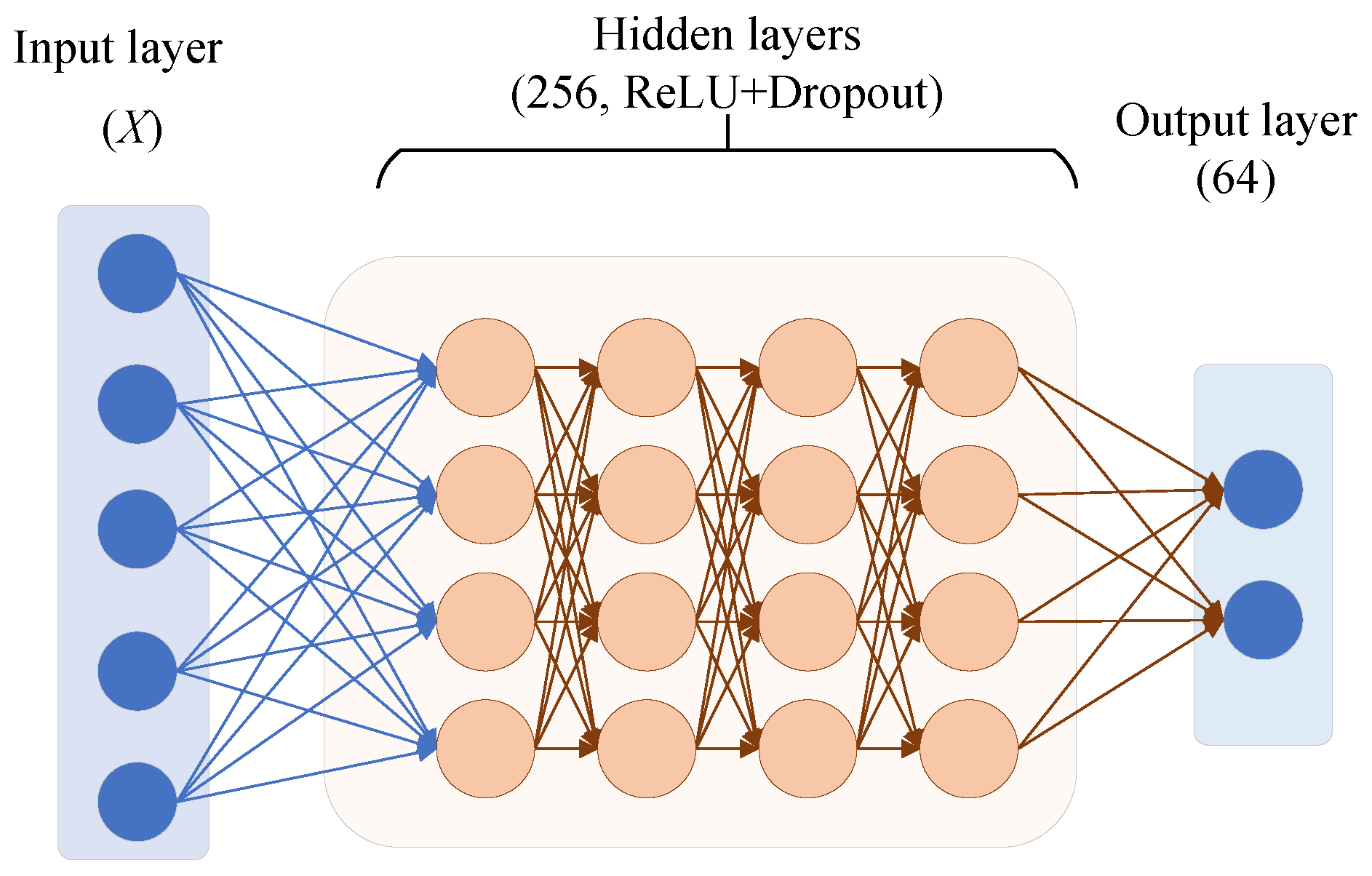
The encoder is a core component of the AutoDAP model. Its primary responsibility is to map the preprocessed high-dimensional user feature data X into a compact and information-rich low-dimensional latent space, generating the latent representation Z. This process aims to automatically extract deep, more discriminative features from user behavior patterns. The encoder employs a Multi-Layer Perceptron (MLP) [36] structure, with its detailed construction shown in Figure 2.

As shown in Figure 2, the encoder’s architecture consists of an input layer, a series of well-designed hidden layers, and an output layer that produces a fixed-dimension latent vector:

• Input Layer. The encoder’s input layer directly accepts the user feature matrix X, which has been preprocessed and standardized as described in Section 3.2.1. This matrix encapsulates each user’s original interaction information and derived statistical features.
• Hidden Layers (4 layers). The encoder contains four hidden layers that progressively abstract and reduce the dimensionality of the input features. Its structure is defined as: $\mathrm{Linear}(n+3\to 256)+\mathrm{ReLU}+\mathrm{Dropout}\left(0.5\right)+\left[\mathrm{Linear}(256\to 256)+\mathrm{ReLU}+\mathrm{Dropout}\left(0.5\right)\right]\times 3$. The uniform width facilitates capacity control and stable training. ReLU provides non-linear representation, while Dropout mitigates overfitting on sparse dimensions.
• Output Layer. A final $\mathrm{Linear}(256\to 64)+\mathrm{ReLU}$ operation produces the 64-dimensional latent vector Z. This vector represents the condensed essence of user behavior patterns learned by the encoder. It is designed to capture crucial information for distinguishing between genuine and attack users in a low-dimensional, dense format. This latent representation Z subsequently serves as input for both the classification and reconstruction tasks. In this way, the encoder effectively achieves its dual objectives of feature dimensionality reduction and key information extraction.

3.2.3. Decoder

The core task of the decoder is to restore (or reconstruct) the original user feature space from the low-dimensional latent vector Z generated by the encoder, obtaining reconstructed features $X^{\prime }$. During model training, the decoder is trained exclusively on the latent representations Z of genuine users. Its goal is to minimize the difference between the reconstructed features $X^{\prime }$ and the original features X of genuine users. This design enables the decoder to focus on learning the intrinsic patterns and distribution of genuine user behavior. When the latent representation of an attack user is fed into the decoder, it is expected to produce a larger reconstruction error, which forms an important basis for detection.

The decoder’s network structure is similar to the encoder’s, also employing an MLP architecture. Its detailed construction is shown in Figure 3:

• Input Layer. Receives the latent vector $Z\in {\mathbb{R}}^{64}$.
• Hidden Layers. The structure is $\mathrm{Linear}(64\to 256)+\mathrm{ReLU}+\mathrm{Dropout}(p=0.4)+\left[\mathrm{Linear}\right(256\to 256)+\mathrm{ReLU}+\mathrm{Dropout}(0.4\left)\right]\times 3$.
• Output Layer. A $\mathrm{Linear}(256\to n+3)$ layer with a linear activation function produces the reconstructed features $X_u^{\prime }$.

Through this structure, the decoder attempts to recover user profile information from the compressed latent representation that is as close as possible to the original input.

3.2.4. Loss Function

To achieve the dual detection objectives proposed in Section 3.1, which are accurately identifying attack users and deeply understanding genuine user behavior patterns, we have carefully designed the following loss function. The total loss ${Loss}_{total}$ is a weighted combination of supervised classification loss and unsupervised reconstruction loss, aiming to synergistically optimize the model’s discriminative and representational learning capabilities.

• Classification Loss Function. The latent representation Z output by the encoder first passes through an additional Sigmoid activation layer. This layer acts as the Classification Head, responsible for predicting the probability $y_u^{\prime }\in [0,1]$ that user u is an attacker. The classification loss ${Loss}_{classify}$ uses Binary Cross-Entropy (BCE) [37] to measure the difference between the predicted probability $y_u^{\prime }$ e and the true label $y_u$ (1 for attack user, 0 for genuine user). To enhance model generalization and prevent overfitting, we introduce an L2 regularization term [38], applied to all trainable weights W in the model. The complete classification loss is defined as:

  $${Loss}_{classify}={Loss}_{BCE}+\lambda {\Vert W\Vert }_2^2.$$

  (9)

  where, $Los{s}_{BCE}$ is calculated as follows:

  $$Los{s}_{BCE}=-{\displaystyle \frac{1}{N}}\sum _{u=1}^N\left[y_{u}log{y}_u^{\prime }+(1-y_u)log(1-y_u^{\prime })\right].$$

  (10)
  Here, N is the number of samples in the current batch. ${\Vert W\Vert }_2^2$ is the L2 norm squared of all trainable model weights W, and $\lambda$ is the regularization coefficient. This loss function considers both prediction accuracy and model complexity, guiding the model to learn more robust user behavior representations.
• Reconstruction Loss Function. The core objective of the reconstruction task is to train the decoder so that it can accurately recover the genuine user’s original input features X from the latent representation Z generated by the encoder. A key design choice is that during decoder training to minimize reconstruction loss, we only use genuine user data from the training set. The rationale is that attack user behavior patterns inherently differ from genuine users. Therefore, when data from these attack users is reconstructed by a decoder optimized for genuine user behavior, a higher reconstruction error than that of genuine users is expected. This becomes an important basis for attack detection. The reconstruction loss $Los{s}_{recon}$ uses Mean Squared Error (MSE) [39] to quantify the deviation between the reconstructed output $x_u^{\prime }$ and the original input $x_u$. It is formally expressed as:

  $$Los{s}_{recon}={\displaystyle \frac{1}{N^{\prime }}}\sum _{u=1}^{N^{\prime }}{\parallel x_u-x_u^{\prime }\parallel }_2^2.$$

  (11)
  Here, $N^{\prime }$ is the number of genuine users involved in reconstruction, $x_u$ is the original feature vector of a genuine user, and $x_u^{\prime }$ is its corresponding reconstructed feature vector.
• Total Loss Function. The model’s total loss ${Loss}_{total}$ is a weighted sum of the classification loss ${Loss}_{classify}$ and the reconstruction loss $Los{s}_{recon}$. This approach integrates supervised and unsupervised learning signals:

  $$Los{s}_{total}=\alpha ·Los{s}_{classify}+\beta ·Los{s}_{recon}.$$

  (12)
  Here, $\alpha$ and $\beta$ are hyperparameters used to balance the importance of the classification and reconstruction tasks, with $\beta =1-\alpha$. By carefully adjusting these two weights, we can guide the model to achieve an optimal balance between accurately identifying attack users (high classification accuracy) and effectively capturing the distribution of genuine user data (low reconstruction error). This joint optimization strategy enables AutoDAP to learn user behavior features more comprehensively, thereby enhancing its robustness in detecting complex and stealthy poisoning attacks. This method of weighting and combining loss functions from different learning tasks shares a common design philosophy with models that aim to fuse different learning paradigms, such as the model in [32] for data visualization, which uses a mixing coefficient to balance autoencoder and classifier losses.

3.2.5. Discrimination Threshold and Attack Score

After model training and feature representation learning, the final attack detection relies on a clear discrimination mechanism. This section will detail how the key discrimination threshold F is determined during the validation phase, and how a user’s attack score s is calculated and used for discrimination during the testing phase.

• Determining the Discrimination Threshold. During model validation, to obtain the optimal discrimination boundary, we determine a composite discrimination threshold F. This threshold combines the predicted probabilities from the classification task and the error measures from the reconstruction task. First, by maximizing the F1-score on the validation set, we separately determine the optimal classification probability threshold $T_{classify}$ and the percentile $k\%$ for selecting genuine user reconstruction errors.
  Based on $k\%$, the optimal reconstruction error threshold $T_{recon}$ is calculated. Its value is the average reconstruction error of the top $k\%$ genuine users in the validation set, sorted by increasing reconstruction error.
  The final discrimination threshold F is calculated using the following formula:

  $$F=\alpha ·T_{classify}+\beta ·T_{recon}.$$

  (13)
  Here, $\alpha$ and $\beta$ are the optimal loss weights, selected through hyperparameter optimization during the model training and validation phases.
• User Attack Score and Final Discrimination. In the testing phase, for any user to be detected, the model first obtains their classification prediction probability $y^{\prime }$ and reconstruction error e.
  Then, the user’s composite attack score s is calculated:

$$s=\alpha ·y^{\prime }+\beta ·e.$$

(14)

Here, $\alpha$ and $\beta$ are consistent with those in Equation (13). Finally, discrimination is performed according to the following rule:

$$y_c=\left\{\begin{array}{cc}1,\hfill & s>F,\hfill \\ 0,\hfill & s\le F.\hfill \end{array}\right.$$

(15)

Here, $y_c$ represents the final detection result, where 1 indicates an attack user and 0 indicates a genuine user.

3.3. Detection Algorithm

Let $r_u$ and $y_u$ denote user u and their label, respectively, where $y_u$ = 0 or 1 indicates a genuine or attack user. Let ${RSet}_t$, ${RSet}_v$, and ${RSet}_{te}$ denote the training, validation, and test sets. ${RSet}_t$ = $\{{(r_u,y_u)}_n,n=1,2,\dots ,N_{train}\}$, where $N_{train}$ is the number of users in the training set. ${RSet}_v$ = $\{{(r_u,y_u)}_n,n=1,2,\dots ,N_{val}\}$, where $N_{val}$ is the number of users in the validation set. ${RSet}_{te}$ = $\{{(r_u,y_u)}_n,n=1,2,\dots ,N_{test}\}$, where $N_{test}$ is the number of users in the test set. Let H represent the set of candidate hyperparameter settings, where each setting is a combination of values for {$epoch$, $\alpha$, $\beta$, $T_{classify}$, $k\%$} drawn from their respective search spaces. Let ${Set}_c$ denote the detection results. The AutoDAP detection algorithm proposed in this paper is shown in Algorithm  1.

Algorithm 1 Detection Algorithm of AutoDAP.

Input: $RSe{t}_t$, $RSe{t}_v$, $RSe{t}_{te}$, H Output: $Se{t}_c$ Step 1: Data Preparation    (1) Use Equations (3)–(6) to extract the interaction matrix I from the datasets $RSe{t}_t$, $RSe{t}_v$, $RSe{t}_{te}$, and compute the statistical features $IM$, $IV$, and $TIC$.    (2) Use Equation (7) to concatenate the original interaction matrix I with $IM$, $IV$, and $TIC$ to form the user - feature matrix for dataset.    (3) Compute the mean $\mu$ and standard - deviation $\sigma$ for each feature dimension using the training set feature matrix $X_{train}$. Then, perform Z - score normalization on $X_{train}$, $X_{val}$, and $X_{test}$ using $(\mu ,\sigma )$ and Equation (8). Step 2: Hyperparameter Optimization and Model Selection    (1) Initialize the best F1_scor${\mathrm{e}}_{best}=-1$, the best hyperparameter combination $h^{*}=\left\{\right\}$, and the best model parameters $p^{*}=\left\{\right\}$.    (2) For each candidate hyperparameter set $h=\{epoch,\alpha ,\beta ,T_{classify},k\%\}$ in H:      (a) Train the model: Initialize the AutoDAP model (including encoder, decoder, and classification head). Train on $X_{train}$ using the specified number of epochs, classification loss weight $\alpha$, and reconstruction loss weight $\beta$. In each training iteration, compute and backpropagate the total loss $Los{s}_{total}$ as defined in Equation (12). Note that the reconstruction loss $Los{s}_{recon}$ is calculated using only the genuine users in $X_{train}$. The model parameters p are iteratively updated in the direction that minimizes the total loss.      (b) Compute validation threshold: Using the trained model p, compute the reconstruction error threshold $T_{recon}$ based on the genuine users in $X_{val}$, by averaging the reconstruction errors of the top $k\%$ users with the lowest errors. Then, compute the decision threshold F using Equation (13) and the current values of $\alpha$, $\beta$, and $T_{classify}$ from h.      (c) Validate the model: For each user in $X_{val}$, use model p to compute the classification probability $y^{\prime }$ and reconstruction error e, then calculate the attack score s using Equation (14). Perform detection using threshold F and Equation (15), and compute the F1 score.      (d) Update global best: If the current F1_score is better than F1_scor${\mathrm{e}}_{best}$, update F1_scor${\mathrm{e}}_{best}=$ F1_score, $h^{*}=h$, $p^{*}=p$. Step 3: Final Decision Rule    (1) Load the best model parameters $p^{*}$.    (2) Extract the optimal hyperparameters $\{epoch,\alpha ,\beta ,T_{classify},k\%\}$ from $h^{*}$. Use $p^{*}$ and the genuine users in $X_{val}$ to compute the final reconstruction error threshold $T_{recon}$ (average of the lowest $k\%$ reconstruction errors). Then, calculate the final decision threshold F using Equation (13). Step 4: Evaluation on the Test Set    (1) For each user in the preprocessed $X_{test}$, use the best model $p^{*}$ to compute the classification probability $y^{\prime }$ and reconstruction error e, and calculate the attack score s using $\alpha$, $\beta$ and Equation (14).    (2) Use Equation (15) to make a final detection decision for each user. Store the result in $Se{t}_c$ and return it.

3.4. Complexity Analysis

To assess the applicability of AutoDAP in large-scale recommender systems, we analyze its computational complexity. The model’s computational cost mainly stems from the forward and backward propagation of its MLP architecture. Let U be the number of users in a batch, D be the original user feature dimension (primarily determined by the number of items n, so $D\approx n$), H be the hidden layer width, and Z be the encoder’s output dimension.

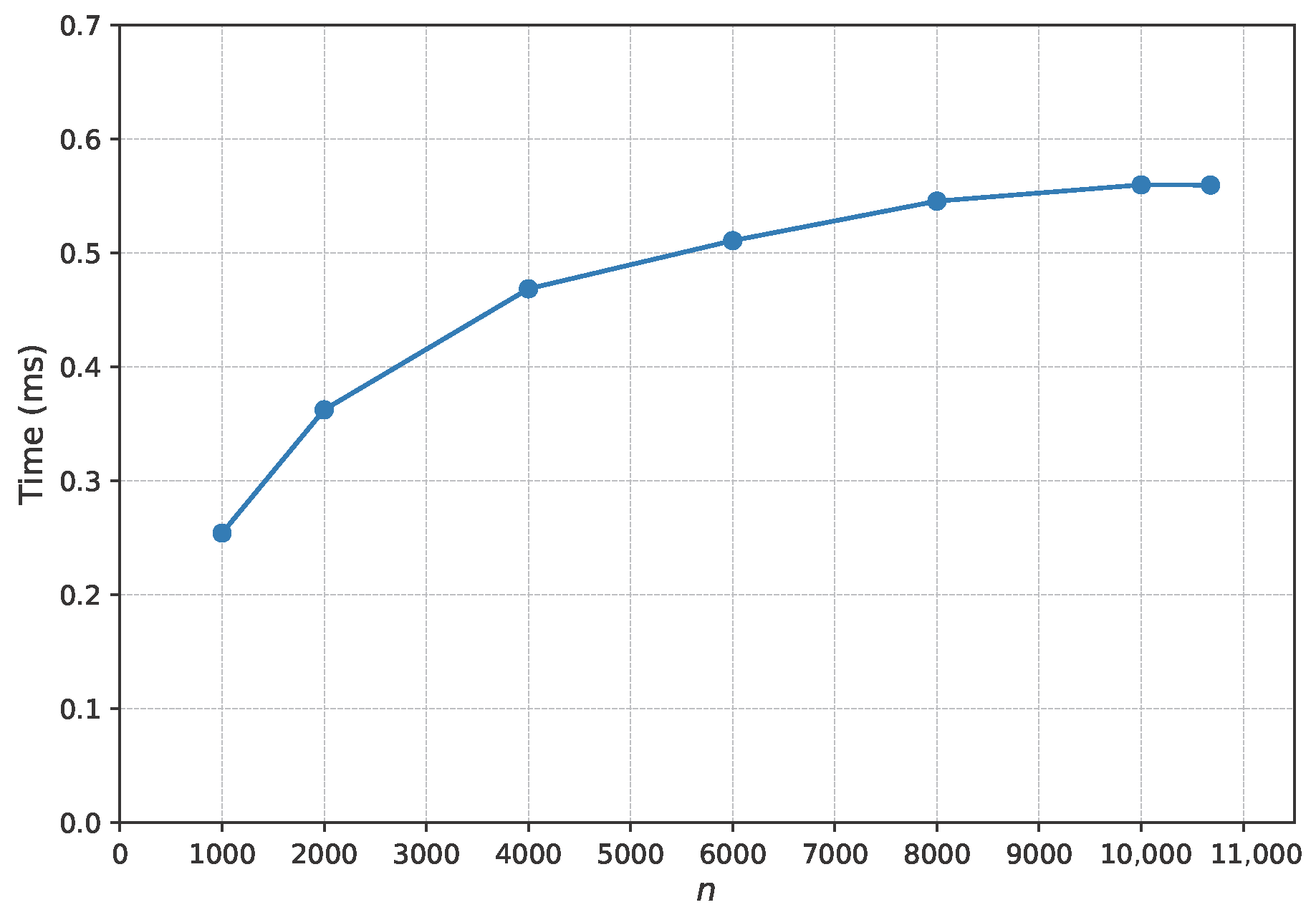
• Training Complexity: The complexity of a single training iteration is determined by both the encoder and the decoder. The encoder’s complexity is $\mathcal{O}(U·(D·H+H^2·L))$, and the decoder’s is $\mathcal{O}(U·(Z·H+H^2·D))$. In practical applications, $D\gg H$ and $D\gg Z$. Therefore, the main contribution to the total training complexity comes from the input and output layers, which can be approximated as $\mathcal{O}(U·D·H)$. This indicates that the training cost is linear with respect to the number of users and items, ensuring the model’s scalability for large datasets. Notably, our dual-objective design only introduces a constant-level of additional computation (for the decoder part) and does not change the order of complexity.
• Inference Complexity: Detecting a single user requires only one forward pass, with a complexity of $\mathcal{O}(D·H)$. The computational cost is extremely low, fully meeting the real-time requirements for online or near-online detection.

In summary, AutoDAP maintains a highly controllable linear computational complexity while ensuring strong detection capabilities, making it suitable for deployment in industrial-grade recommender systems.

3.5. Overfitting Control and Regularization

When processing high-dimensional and sparse user interaction data, deep models face a significant risk of overfitting. To ensure AutoDAP’s generalization ability, we designed and implemented a multi-level, systematic set of regularization strategies, from model architecture to the training process.

First, we incorporated intrinsic constraints at the architectural level. On one hand, through an information bottleneck design, the encoder compresses high-dimensional input into a low-dimensional latent space ($H\ll D$). This forces the model to learn the most core and representative features, naturally suppressing overfitting to noise and sparse artifacts. On the other hand, we use parameter sharing and a dual-task constraint, where the classification and reconstruction tasks share the same encoder. This design compels the encoder to learn a universal representation that is both discriminative and generative. The synergistic constraint of the dual tasks acts as a powerful regularizer, preventing the model from “over-optimizing” for a single task.

Second, we implemented explicit controls at the training optimization level. At the parameter level, we use L2 Regularization (weight decay) to penalize large weight parameters, encouraging the model to learn smoother and simpler decision boundaries. We also apply Dropout between the MLP’s hidden layers, randomly deactivating neurons to reduce complex co-adaptations and enhance model robustness. At the process level, we employ Early Stopping. We select the best model checkpoint based on the F1-score on the validation set, rather than training until convergence. This effectively prevents the model from overfitting to the training data in later stages.

By combining the intrinsic constraints of the architecture with explicit controls during training, AutoDAP can effectively suppress overfitting and learn robust user behavior representations with strong generalization capabilities.

4. Experiments and Analysis

To comprehensively evaluate the performance of AutoDAP in detecting poisoning attacks in GRSs, this section details our experimental setup. We describe the datasets, baseline methods, and evaluation metrics used. We then present and analyze the experimental results under various attack scenarios to validate our method’s effectiveness and robustness.

4.1. Datasets

This study uses two public datasets, MovieLens-10M [40] and Amazon [41], to validate the proposed method’s effectiveness in detecting GRS poisoning attacks. The MovieLens-10M dataset originally contains only genuine users. To create attack scenarios, we use four mainstream GRS poisoning attack models (OGPAttack, GSPAttack, AutoAttack, InfoAtk) to generate attack user data and inject it into this dataset. In contrast, the Amazon dataset already contains genuine users and a portion of identified attack users. To ensure data quality, we removed users with zero ratings from the datasets. Detailed statistics of the processed datasets are shown in

Table 1. Statistics of Experimental Datasets.

Dataset	User	Item	Rating	Rating Range	Filler Ratio	Genuine User	Attack User
MovieLens-10M	71,567	10,681	10,000,054	[0.5–5]	1.34%	71,567	0
Amazon	4902	16,885	51,346	[1–5]	0.06%	2995	1907

.

4.2. Experimental Data Setup

We designed detailed attack injection strategies for the MovieLens-10M dataset, creating diverse attack scenarios by combining different Attack Sizes (ratio of attack users to genuine users) and Filler Sizes (ratio of rated items to total items). For the Amazon dataset, we utilized its inherent attack users to evaluate the method’s detection capability in real-world attack scenarios.

4.2.1. Data Setup on MovieLens-10M Dataset

From the MovieLens-10M dataset, we randomly sampled 1000 genuine users without replacement to build the training, validation, and test sets. For the training set, we used four attack models: OGPAttack, GSPAttack, AutoAttack, and InfoAtk. Under each attack model, for five different filler sizes $\{1\%,1.5\%,3\%,7\%,10\%\}$, we generated 10 attack users each and injected them into the training set. The detailed composition is shown in

Table 2. Training Set Data Setup.

Attack Model	Genuine User	Filler Size
		1%	1.5%	3%	7%	10%
OGPAttack	1000	10	10	10	10	10
GSPAttack	1000	10	10	10	10	10
AutoAttack	1000	10	10	10	10	10
InfoAtk	1000	10	10	10	10	10

.

For the validation set, we used the same attack models and filler size settings as the training set. That is, for each of the four attack models and five filler sizes, 10 attack users were generated and injected into the validation set. The detailed composition is shown in

Table 3. Validation Set Data Setup.

Attack Model	Genuine User	Filler Size
		1%	1.5%	3%	7%	10%
OGPAttack	1000	10	10	10	10	10
GSPAttack	1000	10	10	10	10	10
AutoAttack	1000	10	10	10	10	10
InfoAtk	1000	10	10	10	10	10

.

For the test set, to evaluate model performance more comprehensively, we also used the four attack models mentioned above and designed more complex attack combinations: filler sizes were set to $\{1\%,1.34\%,1.5\%,3\%,7\%,10\%\}$(six types), and attack sizes were set to $\{1\%,3\%,5\%,7\%,9\%,10\%,20\%\}$(seven types). Thus, a total of 4 (attack types) × 6 (filler sizes) × 7 (attack sizes) = 168 different test scenarios were constructed. It is worth noting that we included 1.34% as a filler size in testing. This value was determined based on the actual average sparsity of the MovieLens-10M dataset, aiming to increase detection difficulty by simulating challenging scenarios where attack data has similar sparsity characteristics to genuine user behavior.

4.2.2. Data Setup on Amazon Dataset

For the Amazon dataset, we similarly used random sampling without replacement to partition users into training, validation, and test sets. The number of genuine and attack users in each subset is shown in

Table 4. Number of Users in Each Dataset Split for Amazon.

Dataset Type	Genuine Users	#Attack Users
Training Set	1500	1000
Validation Set	495	407
Test Set	1000	500

.

4.3. Baseline Methods

We selected the following representative recommender system poisoning attack detection methods for comparison. These methods span different technical approaches from traditional machine learning to deep learning, providing a multi-dimensional reflection of the current research landscape.

• FAP [13]. This method is based on the observation that user fraudulent behavior propagates in a network. It constructs a user–item graph and uses a label propagation-like mechanism to identify attack users. This method is representative of early efforts because it attempts to detect attacks from the perspective of behavioral pattern diffusion, enabling generic detection of different attack types and providing early insights for subsequent research.
• Pop-SAD [19]. This method innovatively shifts the focus of poisoning attack detection from traditional “rating patterns” to analyzing users’ “item selection behavior.” Its core insight is that attackers, to achieve their goals, have item selection strategies significantly different from normal users’ preference-based selections. This difference is reflected in their rated item popularity distributions. Thus, Pop-SAD represents a new approach to identifying malicious users by analyzing intrinsic characteristics of user item selection behavior, offering a more robust and computationally cheaper way for attack detection.
• kNN-Mix [20]. This is a mixed-feature detection framework for multi-criteria recommender systems. It combines traditional behavioral features with novel item popularity features and uses a kNN-Mix classifier for attack detection. Its representativeness lies in enhancing detection performance for specific recommender system scenarios (multi-criteria) through carefully designed mixed feature engineering, showcasing innovation in traditional machine learning at the feature level.
• DL-DRA [25]. This method proposes a 2D feature reconstruction-based convolutional detection model. Its core idea is to transform user rating vectors into approximate 2D “images” (square matrices) using techniques like bicubic interpolation, making them suitable for CNN input. This allows CNNs to extract spatial features. This method represents an early attempt to apply mature image processing CNN models to recommender system attack detection, focusing on how to transform data for CNN feature extraction.
• CNN-LSTM [26]. This method designs a spatio-temporal joint learning architecture. The CNN module extracts local spatial patterns in user–item interactions, while the LSTM module models long-term temporal dependencies in user behavior sequences. By combining these two networks, the model can learn implicit feature vectors from user rating data to distinguish between genuine and attack users. This architecture represents a common hybrid model approach in deep learning, aiming to capture both local spatial and sequential temporal characteristics of data.
• SpDetector [27]. This method effectively captures shilling attacks by constructing multiple components such as user spectral features, item similarity offset, and rating prediction error. It then uses these carefully designed features to train a deep learning network for detection. Its representativeness lies in not solely relying on end-to-end automatic feature learning but combining domain knowledge for multi-angle feature engineering, then using a deep learning model for classification, reflecting a strategy that combines feature engineering with deep learning.
• CNN-BAG [28]. This method combines deep learning with ensemble learning. It uses CNN-based deep neural networks as base classifiers to automatically extract and learn shilling attack features. It then employs the Bagging ensemble strategy to improve overall detection performance and robustness. This method represents a research direction that combines the powerful feature representation capabilities of deep learning with the advantages of ensemble learning (e.g., improving stability and generalization) to enhance detection effectiveness.
• CDDPA [33]: An advanced framework for anomalous user detection based on GCN. By employing teacher-student knowledge distillation and contrastive learning, it learns node representations directly from the user–item interaction graph to identify users with atypical topological connection patterns. Its inclusion as a baseline serves to benchmark our method’s competitiveness against a model specifically designed to exploit graph topology.

4.4. Parameter Settings and Evaluation Metrics

We implemented the proposed detection method using PyTorch 2.5.1 (https://pytorch.org/) (accessed on 14 November 2025) and employed the Adam optimizer with a learning rate of 0.001. These are widely used and generally effective configurations in deep learning practice. we used the default PyTorch settings for other parameters.

To achieve optimal model performance, we searched for the following key hyperparameters within their respective ranges: training epoch in [20, 50] (integers); classification loss weight $\alpha$ in [0.1, 0.9] with a step of 0.1, and reconstruction loss weight $\beta$ set to 1−$\alpha$; classification probability threshold $T_{classify}$ in [0.40, 0.60] with a step of 0.01; reconstruction error threshold percentile $k\%$ in [60%, 90%] with a step of 1%. The final reconstruction error threshold, $T_{recon}$, is not searched directly. Instead, it is determined by the optimal $k\%$ found on the validation set. This involves sorting genuine users’ reconstruction errors in the validation set in ascending order and taking the average error of the top $k\%$ users as $T_{recon}$. Hyperparameter optimization used a random search strategy [42], with F1-score on the validation set as the criterion for selecting the best hyperparameter combination.

To ensure fairness and practical relevance, we strictly follow a “train-once, test-all” protocol. Specifically, we train only one AutoDAP model for each dataset. Once its parameters and thresholds are determined on the validation set, the model is fixed. It is then uniformly applied to all test scenarios, regardless of the attack type or size. No re-training or scenario-specific adjustments are made during testing.

We used three standard evaluation metrics widely adopted in recommender system security and classification tasks [5,43]: Recall, which measures the proportion of correctly identified attack users among all actual attack users; Precision, which measures the proportion of actual attack users among samples predicted as attackers; and F1-score, the harmonic mean of Recall and Precision, providing a comprehensive evaluation of both precision and recall. During hyperparameter optimization, we maximized F1-score on the validation set. In the testing phase, to ensure the stability and reliability of evaluation results, we independently generated 5 different test datasets for each test scenario. The final performance of each model is reported as the average of detection results on these 5 independent test datasets.

4.5. Experimental Comparison on MovieLens-10M Dataset

To thoroughly evaluate AutoDAP’s detection performance under different attack scenarios, we conducted extensive experiments on the widely used MovieLens-10M dataset. This section will first introduce the hyperparameter optimization process, then present the detection results of AutoDAP and baseline methods against various types and intensities of poisoning attacks.

4.5.1. Hyperparameter Optimization

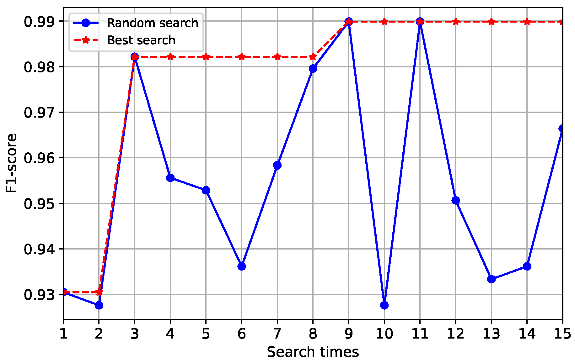
We used F1-score as the evaluation metric and employed a random search strategy on the MovieLens-10M validation set to optimize key hyperparameters. Figure 4 visually demonstrates the F1-score changes corresponding to different hyperparameter combinations during the search process. After multiple search iterations, we found that at the 9th search, when the hyperparameter combination was $\{epoch=20,\alpha =0.7,\beta =0.3,$$T_{classify}=0.51,k\%=75\%\}$, the model achieved the highest F1-score on the validation set. Therefore, this optimal hyperparameter combination was used for all subsequent tests on the MovieLens-10M dataset.

4.5.2. Detection Results

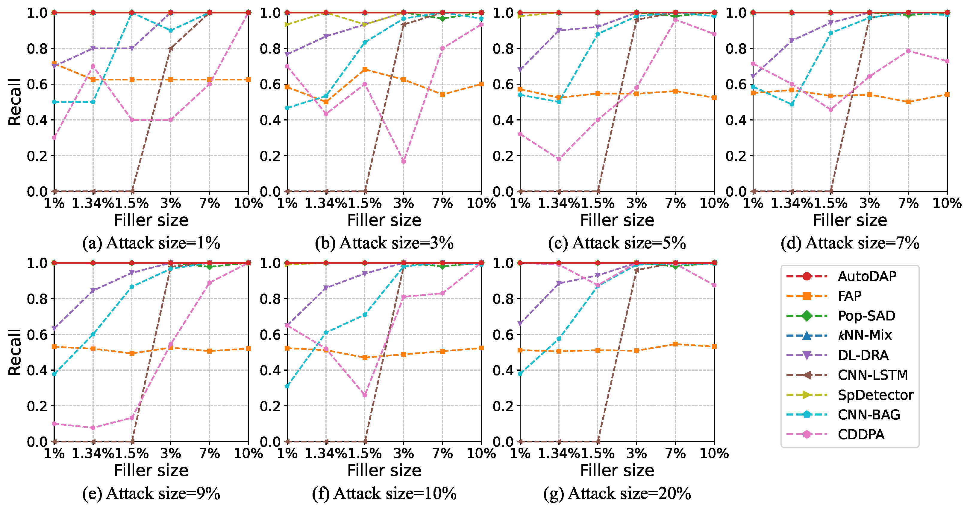
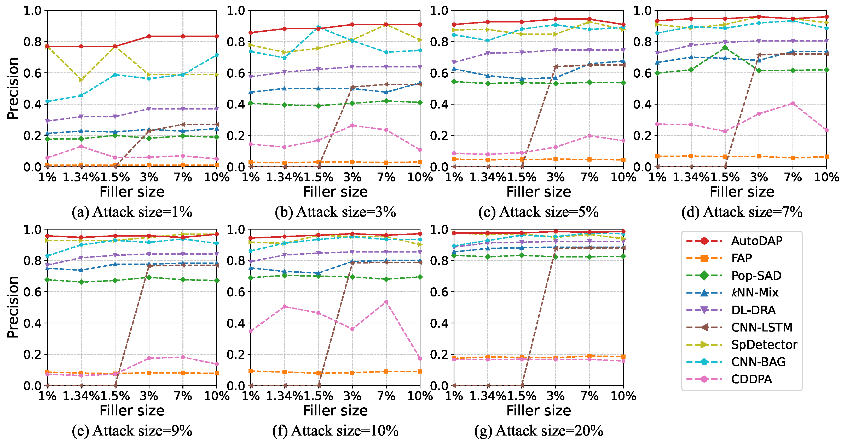
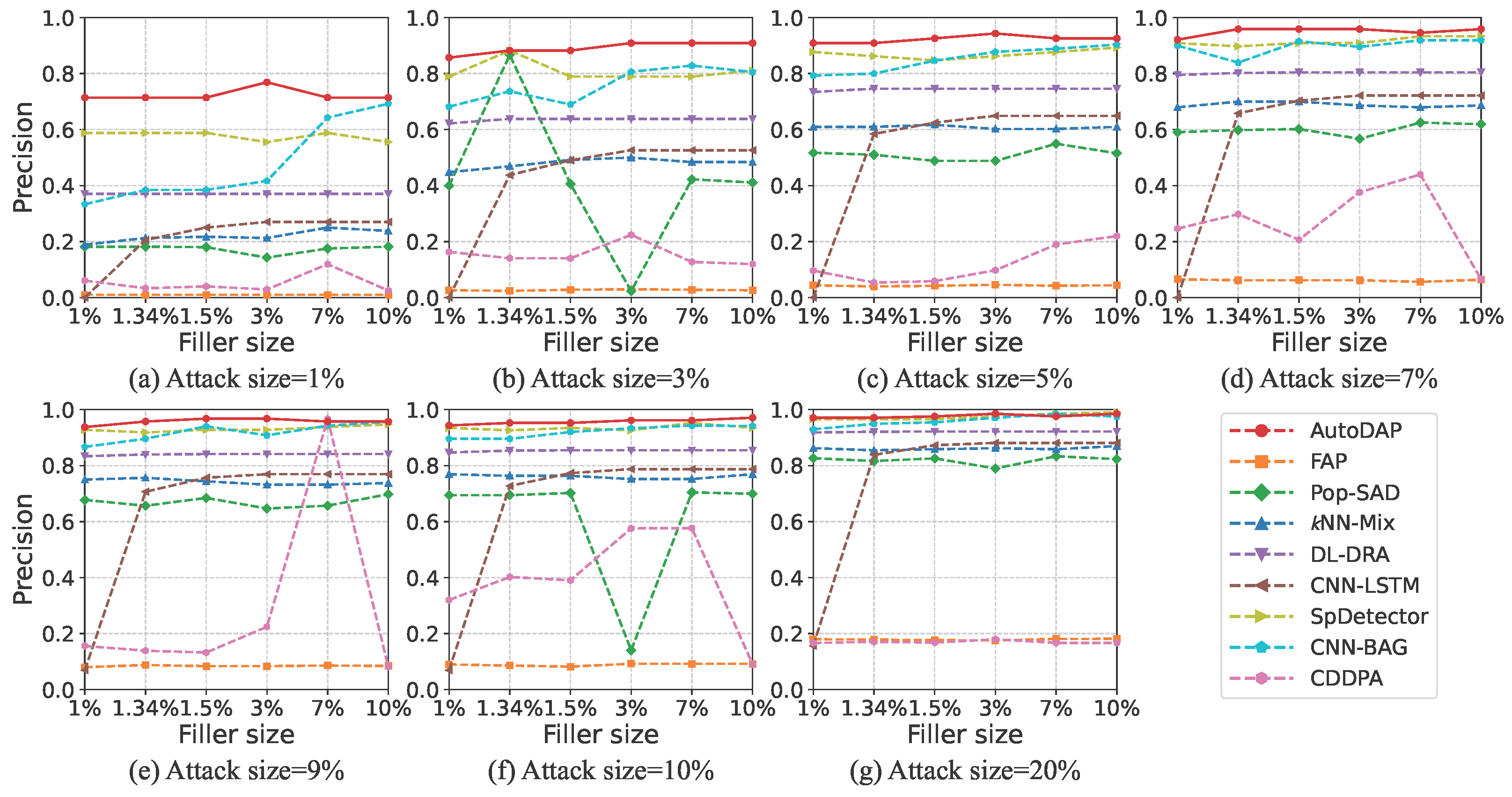
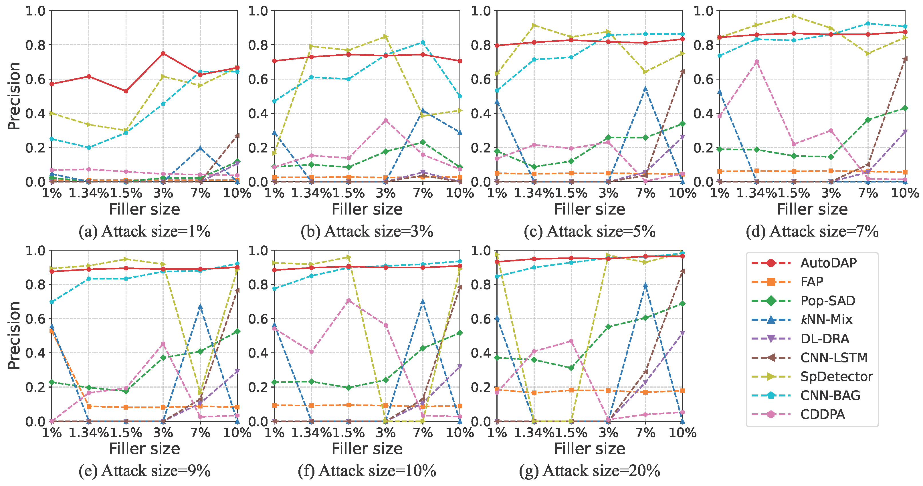
The detection results of various methods on the MovieLens-10M dataset test sets containing OGPAttack are shown in Figure 5, Figure 6 and Figure 7.

OGPAttack is an early optimization-based poisoning attack, aiming to maximize the target item’s hit rate in genuine users’ recommendation lists.

FAP performs poorly, possibly because OGPAttack does not simply mimic “spam information” propagation but has a certain strategy, making FAP’s simple fraud propagation assumption difficult to capture.

CNN-LSTM, CNN-BAG, and DL-DRA show sensitivity to filler size, revealing limitations in their feature extraction capabilities when data is sparse. When user interaction data is insufficient, these models struggle to learn the subtle differences between OGPAttack’s carefully constructed attack patterns and normal patterns from limited local structural or sequential information. Performance improves as data density increases and learnable features become richer.

Pop-SAD and kNN-Mix, being based on statistical or shallow features, show moderate performance. This might be because OGPAttack, while altering local graph structure, may still leave traces in some macroscopic statistical features. However, when attack scale is small or attack user behavior mimics well, these traces are not significant, leading to higher false positive rates.

SpDetector performs relatively well, benefiting from its multi-dimensional feature engineering, capturing OGPAttack-induced anomalies from multiple perspectives like spectral and similarity offsets.

CDDPA’s overall performance is lower than that of AutoDAP and SpDetector. At small to medium filler sizes, its performance curve is low and volatile. It improves slightly as the filler size increases but still does not excel. This is because the method relies on stable graph embeddings and contrastive signals, which are difficult to learn sufficiently under data sparsity and a unified budget. Moreover, OGPAttack does not intentionally maintain embedding consistency, weakening CDDPA’s primary detection criterion.

The proposed AutoDAP demonstrates good performance in this scenario. The key is its autoencoder structure’s ability to learn deeper non-linear representations of data. Through joint optimization of classification and reconstruction losses, AutoDAP not only identifies discriminative features of attack users but also learns a “profile” of genuine user behavior. Even if OGPAttack is optimized, its injected fake interactions still deviate from normal patterns in the deep representation space and are thus effectively detected. This validates our dual-objective approach, where the reconstruction loss component successfully captures deviations from normality that the classification component alone might miss.

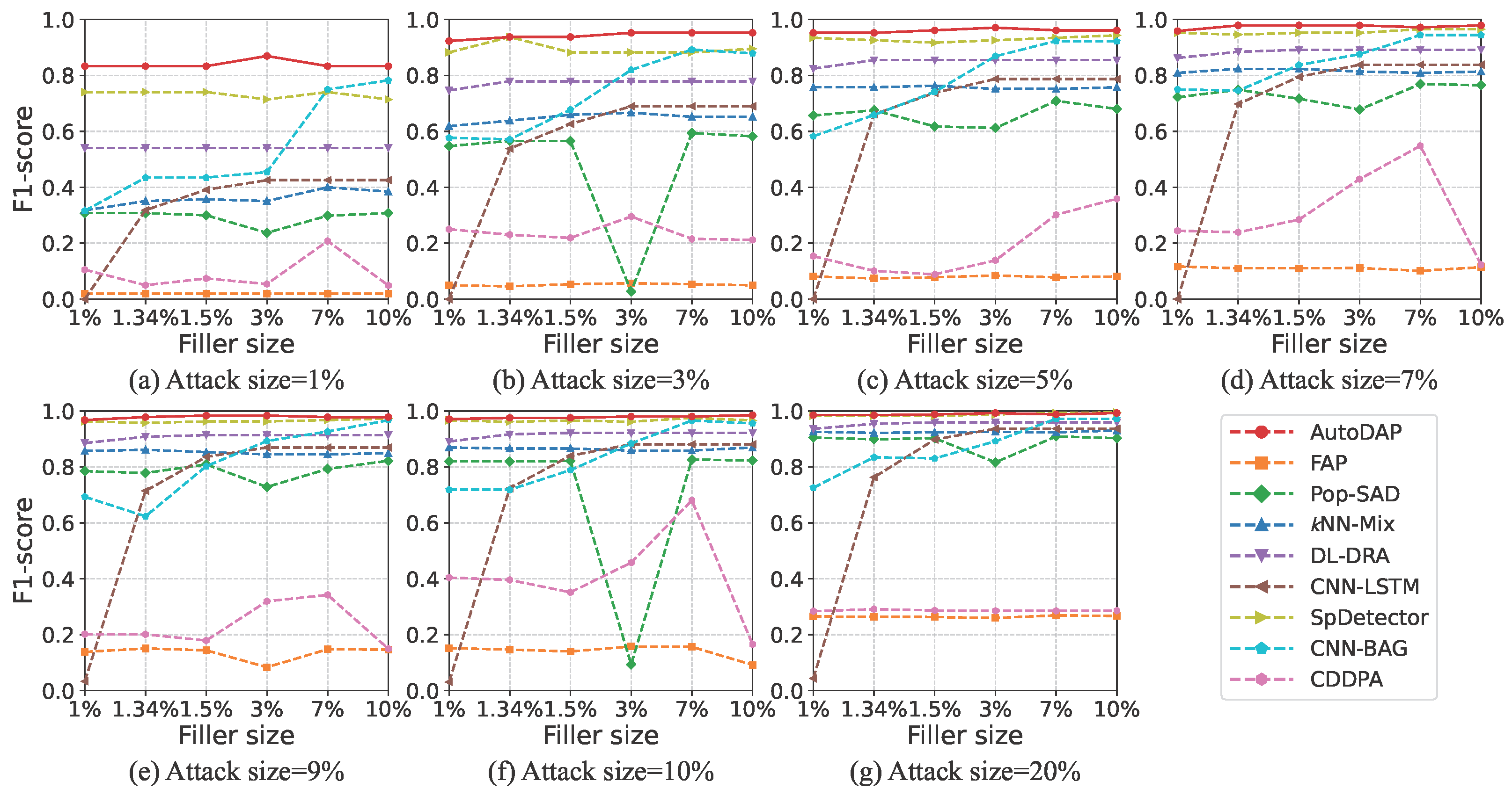
The detection results of various methods on the MovieLens-10M dataset test sets containing GSPAttack are shown in Figure 8, Figure 9 and Figure 10.

GSPAttack uses GAN-like ideas to generate attack users that are harder to detect at the feature level, posing a greater challenge for detection.

The poor performance of FAP and CNN-BAG reflects GSPAttack’s high stealthiness. FAP’s simple assumptions are inadequate, while CNN-BAG’s convolutional kernels may struggle to capture GSPAttack’s subtle, deceptive perturbations in local interaction patterns, especially with small rating coverage where effective signals are scarce.

Pop-SAD’s performance drops at specific filler sizes, indicating GSPAttack can sometimes effectively mimic genuine users’ macroscopic statistical distributions, causing methods based on such statistical anomalies to fail.

CNN-LSTM’s weakness with sparse data further confirms deep models’ reliance on data volume. Fake interactions generated by GSPAttack might mimic genuine users even sequentially, making it hard for the model to distinguish with insufficient data.

The relatively good performance of kNN-Mix and DL-DRA might stem from GSPAttack, despite its feature-level stealth, still introducing “artifacts” in high-dimensional interaction space or transformed representation space that these methods can capture. For example, DL-DRA’s 2D reconstruction might amplify some subtle patterns.

SpDetector’s advantage lies in its comprehensive judgment; GSPAttack might mimic well in one feature dimension but struggle to be perfect across all dimensions.

With small filler sizes, CDDPA’s recall is unstable and prone to misdetection. As the filler size increases, its recall rises significantly, approaching the upper limit at large attack sizes. However, its overall Precision is low. It is more susceptible to misclassifications due to the “realistic” camouflage of generative attacks. This results in a moderate F1-score that is sensitive to the filler size.

AutoDAP’s consistent lead highlights the value of its unsupervised reconstruction capability. Even if users generated by GSPAttack are hard to distinguish by supervised classification features, their inherent “unnaturalness” leads to large reconstruction errors when attempting to reconstruct through a decoder that has learned “normal patterns,” thus being identified. This combination of supervised and unsupervised learning is particularly effective for detecting generative attacks.

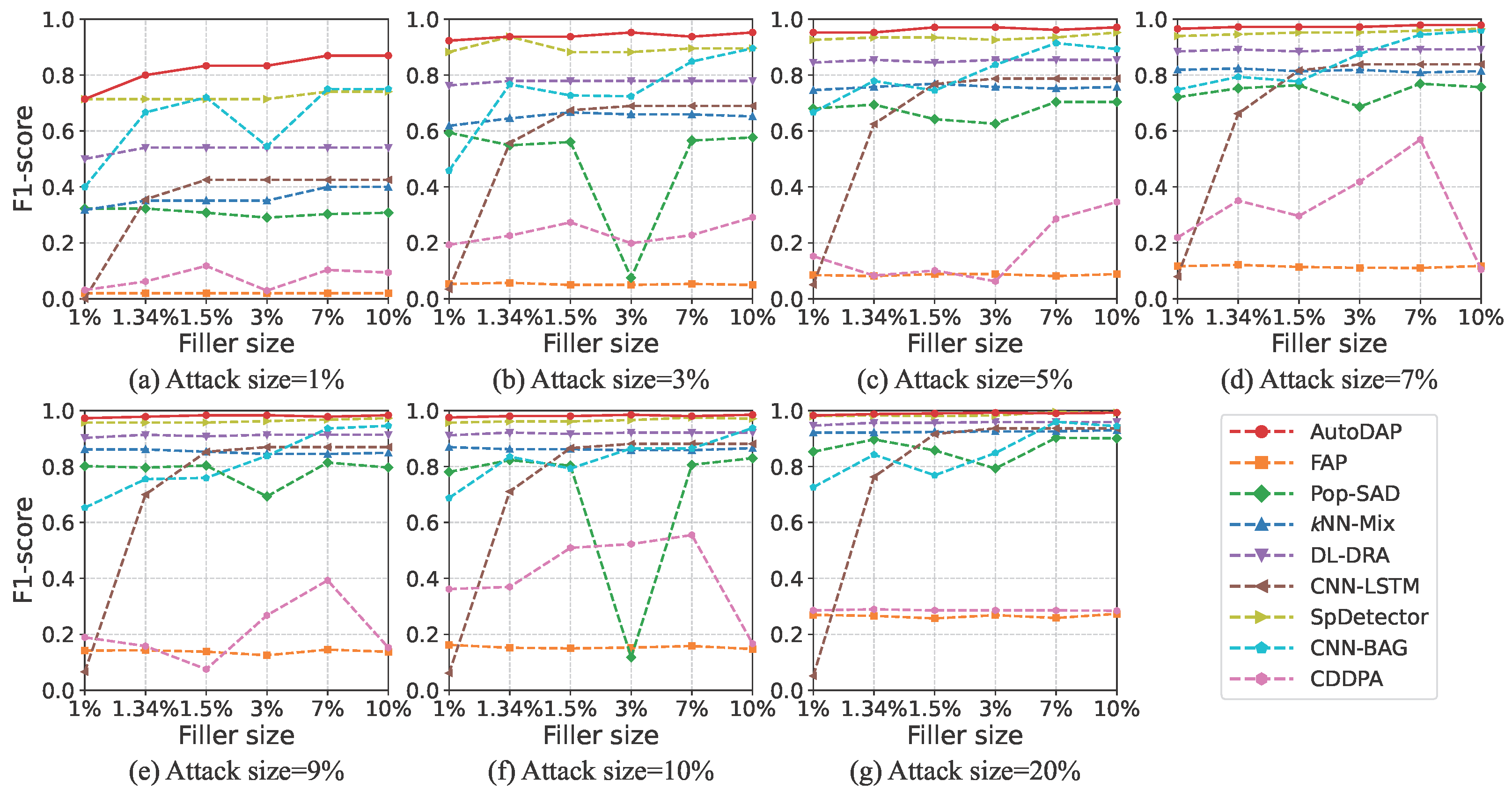
The detection results of various methods on the MovieLens-10M dataset test sets containing AutoAttack are shown in Figure 11, Figure 12 and Figure 13.

AutoAttack is a more advanced automated targeted attack, emphasizing attack precision and similarity to the target user group.

CNN-BAG’s fluctuations with small attack scales may reflect limitations of ensemble learning when base classifiers lack diversity or perform poorly individually. Small-scale attacks might lead to less prominent attack features in training samples, affecting base classifier training.

Pop-SAD’s Precision drops with small attack scales because AutoAttack, in its design, tries to make injected users statistically similar to the target group. This makes detection methods based on macroscopic statistical differences more prone to misclassification when attack signals are weak.

CNN-LSTM’s unstable performance might be related to the diversity of AutoAttack’s attack patterns. Targeted attacks might employ slightly different strategies for different users, making LSTMs based on fixed sequential patterns struggle to adapt.

At low filler sizes, CDDPA’s recall is significantly low and volatile. After a 7% filler size, its recall begins to rise noticeably. However, its Precision and F1-score remain low, lagging significantly behind AutoDAP and SpDetector. When the perturbation signal is weak, CDDPA’s embedding consistency constraint can easily “pull” camouflaged samples back to the normal manifold, leading to misdetection. As the perturbation strengthens, separability increases and recall improves, but its Precision is limited by the deviation between its surrogate objective and the actual detection task.

The excellent performance of SpDetector and AutoDAP indicates they can capture deep anomalies still present in AutoAttack despite its high mimicry. For AutoDAP, the latent representation space learned by its encoder can effectively distinguish carefully designed attack users from genuine users. Even if attack users are similar to target users at the original feature level, their trajectories in high-order interaction patterns or the latent space mapped by the autoencoder might still deviate from genuine user clusters. AutoDAP, by minimizing genuine users’ reconstruction error, makes this deviation more pronounced for attack users.

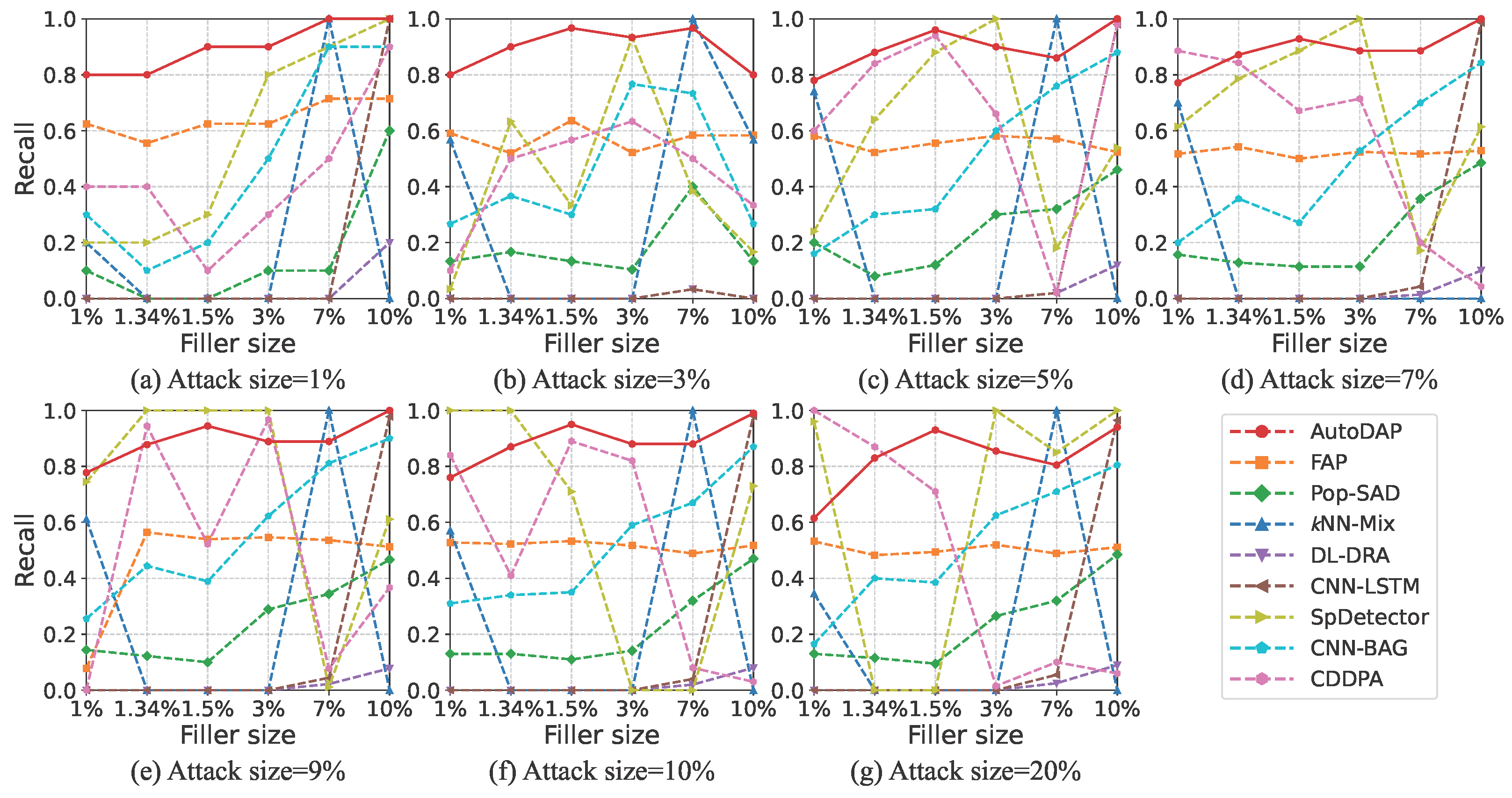
The detection results of various methods on the MovieLens-10M dataset test sets containing InfoAtk are shown in Figure 14, Figure 15 and Figure 16.

InfoAtk elevates attack stealthiness to a new level by using techniques like contrastive learning to minimize differences in user/item embedding representations before and after the attack, posing a severe challenge to detectors. The general performance degradation of all methods directly attests to InfoAtk’s effectiveness. By aligning embeddings, InfoAtk makes attacks “invisible” in the semantic space learned by models, rendering traditional methods based on rating or simple structural anomalies almost entirely ineffective.

The poor performance of CNN-LSTM, Pop-SAD, FAP, and DL-DRA indicates that their relied-upon features or learning mechanisms cannot penetrate InfoAtk’s stealth layer. For instance, original rating pattern differences relied upon by DL-DRA might be masked by InfoAtk’s embedding alignment.

The instability of SpDetector and kNN-Mix reflects that InfoAtk might exhibit different “stealth” effects on different data subsets or specific attack parameters, causing methods relying on fixed feature combinations to fluctuate in performance.

CNN-BAG’s relatively good performance might be due to its ensemble strategy offering some resistance to single-model failure, and its convolutional structure might still capture some high-order local patterns that InfoAtk failed to completely erase.

CDDPA’s Recall is at a moderate level but shows significant fluctuation. At large attack sizes, its Recall trends downward as the filler size increases. Its Precision remains in the low-to-medium range long-term. At larger attack sizes, it begins to fluctuate significantly and decreases as filler size grows, leading to a low and unstable F1-score. This indicates that CDDPA is more sensitive to the feature weakening caused by high stealthiness and is more dependent on sample density, making it difficult to stably capture residual anomalies after embedding alignment.

AutoDAP maintains the best performance even against this highly stealthy attack. Its core advantage lies in its modeling of “normality.” While InfoAtk can make attacks stealthy in specific embedding spaces, completely mimicking all behavioral patterns and intrinsic consistency of genuine users is extremely difficult. AutoDAP’s reconstruction component is dedicated to learning this intrinsic consistency. When interactions injected by InfoAtk deviate from this learned “normal manifold,” they will produce large reconstruction errors even if they are not obvious in discriminative features. Simultaneously, the classification branch can still capture residual attack signals from statistical features and original interactions. This dual mechanism makes AutoDAP more resilient against highly stealthy attacks.

In summary, the proposed AutoDAP method, through its unique autoencoder architecture and dual learning objectives combining supervised classification and unsupervised reconstruction, can learn more robust and deep feature representations from data. This enables it not only to effectively identify traditional and optimized poisoning attacks but also to exhibit good detection performance and generalization ability when facing generative, targeted, and highly stealthy advanced attacks. Its profound understanding and modeling of genuine user behavior patterns are key to maintaining its advantage in complex attack scenarios.

4.6. Experimental Comparison on Amazon Dataset

To further validate AutoDAP’s effectiveness on real-world datasets, especially in handling scenarios containing actual attack samples, we conducted experimental evaluations on the Amazon dataset. This dataset naturally includes a portion of identified attack users, providing a testbed closer to practical application environments.

4.6.1. Hyperparameter Optimization

Similar to the process for the MovieLens-10M dataset, we also performed random search hyperparameter optimization on the Amazon dataset’s validation set, using F1-score as the objective. Figure 17 shows its optimization process. Ultimately, we selected the hyperparameter combination $\{epoch=27,\alpha =0.7,\beta =0.3,T_{classify}=0.59,k\%=72\%\}$, which performed best on the validation set (found at the 12th search iteration), for subsequent testing.

4.6.2. Detection Results

Figure 18 shows the Recall, Precision, and F1-score of AutoDAP and baseline methods on the Amazon test set.

As shown in Figure 18, traditional methods like FAP, Pop-SAD, and kNN-Mix perform significantly worse than most deep learning methods on this real-world dataset. This suggests their limited capability in handling real, complex attack patterns. Although CDDPA achieves the highest recall, its F1-score is low, even underperforming traditional methods. Among all deep learning methods, the proposed AutoDAP achieves the best performance on all three evaluation metrics. Its Recall, Precision, and F1-score all exceed 0.9. This result strongly validates AutoDAP’s ability to efficiently and accurately identify attack users in complex environments with real attack data, demonstrating its superior generalization ability and practical application potential.

4.7. Ablation Study

We conducted an ablation study to investigate the contribution of the three statistical features ($IM$, $IV$, and $TIC$) introduced in Section 3.2.1 to the model’s detection performance. These features aim to capture user behavior patterns at a macroscopic level, serving as complementary information to the original interaction matrix input into the autoencoder.

The ablation study was performed on both MovieLens-10M and Amazon datasets, which have different characteristics. On the MovieLens-10M dataset, we selected an intermediate scenario with an attack size of 7% and a filler size of 3% for testing. In this scenario, we compared the performance of the AutoDAP model with these three statistical features (i.e., the complete model) versus without them (using only the original interaction matrix as input). We evaluated the models against the OGPAttack, GSPAttack, AutoAttack, and InfoAtk attack types. On the Amazon dataset, since it inherently contains identified attack users, we directly compared the performance of the complete model versus the model without statistical features in detecting these real attack users. Experimental results are shown in

Table 5. Ablation study results for the three proposed statistical features. Performance improvements are indicated by underlined numerical values.

Data Set	Attack Model	Without Statistical Features			With Statistical Features
		Recall	Precision	F1-Score	Recall	Precision	F1-Score
MovieLens-10M	OGPAttack	1.0000	0.9459	0.9722	1.0000	0.9589	0.9790
	GSPAttack	1.0000	0.9452	0.9718	1.0000	0.9589	0.9790
	AutoAttack	1.0000	0.9459	0.9722	1.0000	0.9459	0.9722
	InfoAtk	0.6286	0.9362	0.7521	0.8857	0.8611	0.8732
Amazon	Identified attack user	0.9380	0.9214	0.9296	0.9380	0.9269	0.9324

.

For AutoAttack, the presence or absence of statistical features had little impact on model performance, with all metrics remaining largely unchanged. This might imply that AutoAttack, in its design, has already sufficiently considered these basic statistical features for mimicry, reducing the discriminative power of these three features. AutoDAP at this point relies more on deep patterns learned from the original interaction data.

Interestingly, under the InfoAtk attack, while adding statistical features increased Recall and F1-score, it also led to a slight decrease in Precision. This suggests that for such highly stealthy attacks, these macroscopic statistical features might be a “double-edged sword”: they might help identify some more concealed attack users (improving Recall), but also, because attack users mimic these statistical features too well, even surpassing some genuine users’ statistical profiles, they might introduce a small number of new misclassifications (reducing Precision). Nevertheless, the overall F1-score improvement indicates their positive effect still dominates.

For the Amazon dataset, when detecting identified attack users, the model’s Precision and F1-score both showed some improvement after adding the three statistical features. This further confirms the effectiveness of these macroscopic statistical features in real, complex attack scenarios. Real-world attack user behavior patterns are diverse, and these statistical features can capture abnormal signals from a broader perspective, assisting the model in making more accurate judgments.

In summary, the ablation study results strongly validate the positive role of introducing the three statistical features, $IM$, $IV$, and $TIC$, in the AutoDAP model. Although their benefit might not be obvious for certain attacks that extremely mimic statistical features (like specific configurations of AutoAttack), in most GRS poisoning attack scenarios, especially against OGPAttack, GSPAttack, and real attacks on the Amazon dataset, these features effectively supplement the original interaction information. They provide crucial macroscopic behavioral clues, thereby effectively improving the model’s detection accuracy and overall performance. This validates that in designing attack detection systems, combining domain knowledge to extract effective auxiliary features with deep learning models automatically learning deep representations is an effective strategy.

4.8. In-Depth Analysis

After confirming the superiority of AutoDAP over baseline models, this section provides an in-depth analysis of its intrinsic properties and performance boundaries. Through a series of diagnostic experiments, we systematically answer four key questions:

• How robust is the model to key hyperparameters?
• Is the model’s performance stable against random data perturbations?
• What are the performance limits when facing state-of-the-art, highly stealthy attacks?
• Can the attack pattern recognition ability learned from a source domain generalize to a new target domain?
• How does the model perform in terms of computational efficiency and scalability in practical applications?

4.8.1. Sensitivity Analysis

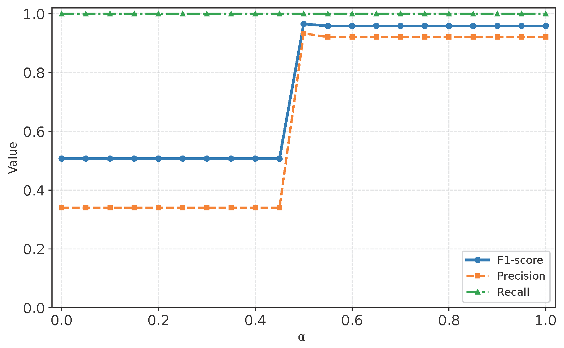
An ideal detection model should not have its performance overly dependent on fine-tuning key hyperparameters. This section evaluates AutoDAP’s sensitivity to its core hyperparameter—the fusion weight $\alpha$ for classification and reconstruction losses. To do this, we fix the trained model parameters and systematically vary $\alpha$ (from 0 to 1) during the inference phase, observing the changes in F1-score, Precision, and Recall on the MovieLens-10M validation set.

The results, shown in Figure 19, clearly reveal the model’s high robustness. When $\alpha$ is small ($\alpha <0.5$), the decision is dominated by reconstruction error, leading to lower precision. However, once $\alpha$ exceeds 0.5, the classification probability begins to dominate the decision. The model’s performance rapidly improves and enters a wide “performance plateau” ($\alpha \in [0.55,1.0]$). Within this range, the F1-score remains near optimal with minimal fluctuation. This finding strongly validates that AutoDAP is not a fragile model requiring meticulous tuning. Its excellent performance is reproducible over a broad range of parameters, greatly enhancing its reliability and ease of use in practical deployments.

4.8.2. Stability Analysis

To verify the stability and reproducibility of the model’s performance and to rule out chance from a single experiment, we conducted a rigorous stability assessment. For each attack scenario on the MovieLens-10M dataset, we independently generated 5 different test sets. The model, trained only once, was evaluated separately on these 5 datasets. We report the mean and standard deviation (mean ± std) of its performance.

The performance data, as shown in

Table 6. Performance stability and robustness of AutoDAP across varying attack sizes. The table presents the mean and standard deviation (mean ± std) of key detection metrics from 5 independent trials, with a fixed filler size of 3%.

Attack Size	Precision (Mean ± Std)	Recall (Mean ± Std)	F1-Score (Mean ± Std)
1%	$0.7477\pm 0.1021$	$1.0000\pm 0.0000$	$0.8524\pm 0.0699$
3%	$0.8997\pm 0.0405$	$1.0000\pm 0.0000$	$0.9468\pm 0.0225$
5%	$0.9337\pm 0.0313$	$1.0000\pm 0.0000$	$0.9655\pm 0.0168$
7%	$0.9543\pm 0.0269$	$1.0000\pm 0.0000$	$0.9765\pm 0.0141$
9%	$0.9619\pm 0.0201$	$1.0000\pm 0.0000$	$0.9805\pm 0.0104$
10%	$0.9675\pm 0.0217$	$1.0000\pm 0.0000$	$0.9834\pm 0.0112$
20%	$0.9853\pm 0.0077$	$1.0000\pm 0.0000$	$0.9926\pm 0.0039$

, demonstrates the model’s exceptional stability. Across all attack sizes, the recall consistently remains at 1.00 with a standard deviation of 0, showing extreme robustness. More importantly, as the attack size increases from 1% to 20%, the standard deviations for both Precision and F1-score show a clear convergence trend, ultimately approaching zero. This “high mean, low variance” performance proves that AutoDAP’s high scores are not due to random luck but are a direct reflection of its powerful and reliable detection capabilities.

4.8.3. Analysis of the Highly Stealthy InfoAtk Attack

The InfoAtk attack, by aligning the representations of attack and normal users in the embedding space, poses an extreme challenge for all detectors and serves as a “touchstone” for testing a model’s performance limits. To comprehensively evaluate AutoDAP in this extreme scenario, we analyzed the Precision–Recall (PR) curve on the MovieLens-10M dataset, which is more informative than a single F1-score. We also used 10-fold bootstrap resampling to quantify the uncertainty of its performance.

The PR curve analysis, as shown in Figure 20, is convincing. The average PR curve is positioned very close to the top-right corner of the plot, indicating that the model can achieve extremely high recall while maintaining extremely high precision. Crucially, the confidence interval around the curve, formed by one standard deviation, is very narrow. These two observations together prove that even when facing the InfoAtk attack, which is designed to fundamentally evade detection, AutoDAP’s “classification + reconstruction” dual-objective architecture can still sensitively capture the residual anomalous signals that cannot be completely erased from its behavior patterns. The model’s performance is not only excellent but also highly stable.

4.8.4. Cross-Domain Generalization Analysis

An essential characteristic of a robust detection model is its ability to generalize to data from different domains. To formally evaluate the domain generalization capability of AutoDAP, we conducted a stringent zero-shot cross-domain transfer experiment.

Experimental Setup: The model trained exclusively on the MovieLens-10M dataset was applied in a zero-shot manner to the Amazon test set. This test is designed to measure out-of-distribution performance, as the Amazon dataset possesses entirely different user and item sets, along with distinct rating distributions and sparsity characteristics. Crucially, no re-training or fine-tuning on the target domain data was performed.

Results and Analysis: The model’s detection performance on the Amazon dataset is presented below: Recall = 0.314, Precision = 0.306, and F1-score = 0.310.

The results indicate that the model’s performance degrades significantly when directly applied to a new and different domain. While the model achieves a non-zero F1-score, suggesting some minimal signal may be captured, the low score of 0.310 clearly illustrates that the representations learned from the MovieLens dataset are not sufficiently general to be effective on the Amazon dataset.

This finding is highly informative, as it establishes a quantitative baseline for the cross-domain challenge in poisoning attack detection. It highlights the model’s current limitations and strongly motivates that future work must focus on developing techniques for domain adaptation—such as feature alignment or adversarial training—to create more portable and practically applicable detection systems.

4.8.5. Computational Efficiency and Scalability Analysis

To supplement the theoretical complexity analysis in Section 3.4 and to validate the practical feasibility of AutoDAP in real-world deployment scenarios, this section empirically evaluates the model’s computational efficiency and scalability. The experiments were conducted on the MovieLens-10M dataset using an NVIDIA RTX 4050 GPU.

First, we examine the model’s training overhead. Since the training process can be fully completed in an offline environment, it has no direct impact on online services. In our experiments, the total training time was a mere 1.27 s. This cost is well within acceptable limits for offline tasks that require rapid iteration and model updates.

For online deployment, inference efficiency is a critical performance metric. We focus on the end-to-end total latency, which includes feature extraction, data normalization, and model inference. To comprehensively assess its performance, we measured the average end-to-end latency per user as the total number of system items, n (a key factor affecting performance), increases. To ensure the stability and precision of the measurements, the latency for each data point was obtained by averaging the results of 1000 repeated detections for a single user. The experimental results are shown in Figure 21.

Two key conclusions can be drawn from the figure:

(1)

Exceptional Real-Time Performance: Across all tested scales, even when the number of items exceeds ten thousand, the total average per-user overhead, including all preprocessing, remains below 0.6 milliseconds. This sub-millisecond latency is significantly lower than the typical industry requirement of tens of milliseconds for online services, fully confirming the model’s capability to meet real-time detection needs.

(2)

Strong Scalability: The total latency exhibits a controllable, non-explosive, sub-linear growth trend as the number of items increases. The slope of the curve flattens with the growing number of items, which indicates that as the system scales up, the marginal time cost for processing each additional item decreases. This demonstrates excellent scalability.

Specifically, at the dataset’s actual scale of 10,678 items, we measured an average end-to-end latency of 0.5597 milliseconds. In summary, these empirical results provide strong evidence that our proposed method possesses both exceptional real-time processing performance and robust scalability, making it fully viable for deployment in large-scale industrial recommender systems.

4.9. Discussion

Through extensive and in-depth experimental evaluations on two representative datasets, MovieLens-10M and Amazon, this paper has comprehensively validated the good performance and robustness of the proposed AutoDAP method in GRS poisoning attack detection tasks. Experimental results clearly show that AutoDAP, when facing various mainstream and emerging poisoning attack types, achieves detection performance that is superior to or on par with existing representative baseline methods across key evaluation metrics.

AutoDAP’s success is primarily attributed to its carefully designed architecture and learning mechanism. First, unlike traditional machine learning methods that rely on time-consuming and labor-intensive handcrafted features, AutoDAP leverages the powerful capabilities of autoencoders. It automatically learns deeper, more discriminative latent representations from raw user interaction data and auxiliary statistical features, effectively overcoming the limitations of handcrafted feature engineering. Secondly, AutoDAP innovatively combines supervised learning classification tasks with unsupervised learning reconstruction tasks. It achieves synergistic enhancement through joint loss function optimization: the classification branch directly learns the decision boundary between attack and genuine users, while the reconstruction branch focuses on learning the intrinsic “profile” of genuine user behavior. This allows the model not only to identify obvious attack signals but also to capture, via reconstruction errors, those stealthy attack users who attempt to mimic normal behavior but whose intrinsic patterns still deviate. This dual-pronged approach significantly improves detection sensitivity and generalization ability. Furthermore, although AutoDAP’s input is user feature matrices, its design was explicitly aimed at GRS poisoning attacks. These attacks often manipulate user–item interaction graph topology to affect GNN learning. AutoDAP, through detailed modeling of user interaction behavior (including original interactions and macroscopic statistical features), captures the imprints left by these graph structural perturbations on user behavior patterns, thereby effectively detecting attacks on graph structures.

Despite these encouraging results, AutoDAP’s utilization of graph structural information is still indirect. The current model primarily infers graph structural perturbations by analyzing user interaction features. An important direction for future research is to explore how to more directly integrate the powerful graph representation learning capabilities of GNNs to further improve detection performance.

5. Conclusions and Future Work

Addressing the increasingly severe threat of poisoning attacks faced by GRSs, this paper proposed AutoDAP, a novel detection method. The core of its success lies in an innovative dual-objective architecture that synergistically combines supervised and unsupervised learning. By jointly optimizing a classification loss and a reconstruction loss, AutoDAP effectively fuses the discriminative power of supervised signals with the ability to model the normal patterns of genuine users, a capability derived from its autoencoder foundation. This design enables the precise identification of various malicious behaviors that manipulate graph structures. Extensive evaluations on the widely used MovieLens-10M dataset demonstrated AutoDAP’s superior Recall, Precision, and F1-score against a range of mainstream and emerging poisoning attacks, including OGPAttack, GSPAttack, AutoAttack, and InfoAtk. Crucially, experiments on the Amazon dataset, which contains real-world attack data, further validated AutoDAP’s effectiveness and generalization. The results confirm that our method can robustly identify complex poisoning attacks in both simulated and real-world scenarios. Despite these encouraging results, the current model’s utilization of graph structural information is still indirect, primarily inferring perturbations by analyzing user interaction features. An important direction for future research is to explore the direct integration of GNNs. For instance, GNN-extracted node embeddings could serve as richer input features, or an end-to-end GNN-based anomaly detection model could be constructed. Such enhancements would more fully leverage graph topological information, potentially leading to further improvements in detection performance.

References

1. Sheng, Z.; Wei, L. HS-SocialRec: A Study on Boosting Social Recommendations with Hard Negative Sampling in LightGCN. Information 2025, 16, 422. [Google Scholar] [CrossRef]
2. Huang, J.; Xie, Z.; Zhang, H.; Yang, B.; Di, C.; Huang, R. Enhancing Knowledge-Aware Recommendation with Dual-Graph Contrastive Learning. Information 2024, 15, 534. [Google Scholar] [CrossRef]
3. Nguyen, T.T.; Nguyen, Q.V.H.; Nguyen, T.T.; Huynh, T.T.; Nguyen, T.T.; Weidlich, M.; Yin, H. Manipulating Recommender Systems: A Survey of Poisoning Attacks and Countermeasures. ACM Comput. Surv. 2024, 57, 3. [Google Scholar] [CrossRef]
4. Lam, S.K.; Riedl, J. Shilling Recommender Systems for Fun and Profit. In Proceedings of the 13th International Conference on World Wide Web, New York, NY, USA, 17–20 May 2004; Feldman, S., Uretsky, M., Najork, M., Wills, C., Eds.; ACM: New York, NY, USA, 2004; pp. 393–402. [Google Scholar] [CrossRef]
5. Nawara, D.; Aly, A.; Kashef, R. Shilling Attacks and Fake Reviews Injection: Principles, Models, and Datasets. IEEE Trans. Comput. Soc. Syst. 2024, 12, 362–375. [Google Scholar] [CrossRef]
6. Burke, R.; Mobasher, B.; Zabicki, R.; Bhaumik, R. Identifying Attack Models for Secure Recommendation. In Beyond Personalization; Setten, M.V., McNee, S.M., Konstan, J.A., Terveen, L., Ardissono, L., Herlocker, J., Smyth, B., Nijholt, A., Eds.; IUI’05: San Diego, CA, USA, 2005; pp. 347–361. Available online: http://www.grouplens.org/beyond2005/papers.html (accessed on 14 November 2025).
7. Fang, M.; Yang, G.; Gong, N.Z.; Liu, J. Poisoning Attacks to Graph-Based Recommender Systems. In Proceedings of the 34th Annual Computer Security Applications Conference, San Juan, PR, USA, 3–7 December 2018; Caballero, J., Gu, G., Eds.; ACM: New York, NY, USA, 2018; pp. 381–392. [Google Scholar] [CrossRef]
8. Nguyen, T.T.; Quach, N.D.K.; Nguyen, T.T.; Huynh, T.T.; Vu, V.H.; Nguyen, P.L.; Jo, J.; Nguyen, Q.V.H. Poisoning GNN-based Recommender Systems with Generative Surrogate-based Attacks. ACM Trans. Inf. Syst. 2023, 41, 58. [Google Scholar] [CrossRef]
9. Guo, S.; Bai, T.; Deng, W. Targeted Shilling Attacks on GNN-based Recommender Systems. In Proceedings of the 32nd ACM International Conference on Information and Knowledge Management, Birmingham, UK, 21–25 October 2023; Frommholz, I., Hopfgartner, F., Lee, M., Oakes, M., Lalmas, M., Zhang, M., Santos, R., Eds.; ACM: New York, NY, USA, 2023; pp. 649–658. [Google Scholar] [CrossRef]
10. Ma, H.; Gao, M.; Wei, F.; Wang, Z.; Jiang, F.; Zhao, Z.; Yang, Z. Stealthy Attack on Graph Recommendation System. Expert Syst. Appl. 2024, 255, 124476. [Google Scholar] [CrossRef]
11. Chirita, P.A.; Nejdl, W.; Zamfir, C. Preventing Shilling Attacks in Online Recommender Systems. In Proceedings of the 7th Annual ACM International Workshop on Web Information and Data Management, New York, NY, USA, 4 November 2005; Bonifati, A., Lee, D., Eds.; ACM: New York, NY, USA, 2005; pp. 67–74. [Google Scholar] [CrossRef]
12. Mehta, B.; Hofmann, T.; Fankhauser, P. Lies and propaganda: Detecting Spam Users in Collaborative Filtering. In Proceedings of the 12th International Conference on Intelligent User Interfaces, Honolulu, HI, USA, 28–31 January 2007; ACM: New York, NY, USA, 2007; pp. 14–21. [Google Scholar] [CrossRef]
13. Zhang, Y.; Tan, Y.; Zhang, M.; Liu, Y.; Chua, T.S.; Ma, S. Catch the Black Sheep: Unified Framework for Shilling Attack Detection Based on Fraudulent Action Propagation. In Proceedings of the 24th International Conference on Artificial Intelligence, Buenos Aires, Argentina, 25–31 July 2015; Yang, Q., Wooldridge, M., Eds.; AAAI Press: Menlo Park, CA, USA, 2015; pp. 2408–2414. Available online: https://dl.acm.org/doi/10.5555/2832581.2832585 (accessed on 14 November 2025).
14. Zhang, F.; Zhang, Z.; Zhang, P.; Wang, S. UD-HMM: An Unsupervised Method for Shilling Attack Detection Based on Hidden Markov Model and Hierarchical Clustering. Knowl.-Based Syst. 2018, 148, 146–166. [Google Scholar] [CrossRef]
15. Cai, H.; Zhang, F. BS-SC: An Unsupervised Approach for Detecting Shilling Profiles in Collaborative Recommender Systems. IEEE Trans. Knowl. Data Eng. 2019, 33, 1375–1388. [Google Scholar] [CrossRef]
16. Zhang, F.; Chan, P.P.K.; He, Z.M.; Yeung, D.S. Unsupervised Contaminated User Profile Identification Against Shilling Attack in Recommender System. Intell. Data Anal. 2024, 28, 1411–1426. [Google Scholar] [CrossRef]
17. Williams, C.A.; Mobasher, B.; Burke, R. Defending Recommender Systems: Detection of Profile Injection Attacks. Serv. Oriented Comput. Appl. 2007, 1, 157–170. [Google Scholar] [CrossRef]
18. Zhou, W.; Wen, J.; Xiong, Q.; Gao, M.; Zeng, J. SVM-TIA A Shilling Attack Detection Method Based On SVM and Target Item Analysis in Recommender Systems. Neurocomputing 2016, 210, 197–205. [Google Scholar] [CrossRef]
19. Li, W.; Gao, M.; Li, H.; Zeng, J.; Xiong, Q.; Hirokawa, S. Shilling Attack Detection in Recommender Systems Via Selecting Patterns Analysis. IEICE Trans. Inf. Syst. 2016, 99, 2600–2611. [Google Scholar] [CrossRef]
20. Kaya, T.T.; Yalcin, E.; Kaleli, C. A Novel Classification-based Shilling Attack Detection Approach for Multi-criteria Recommender Systems. Comput. Intell. 2023, 39, 499–528. [Google Scholar] [CrossRef]
21. Gambhir, S.; Dhawan, S.; Singh, K. Enhancing Recommendation Systems with Skew Deviation Bias for Shilling Attack Detection. Recent Adv. Electr. Electron. Eng. 2025, 18, 212–233. [Google Scholar] [CrossRef]
22. Wu, Z.; Wu, J.; Cao, J.; Tao, D. HySAD: A Semi-Supervised Hybrid Shilling Attack Detector for Trustworthy Product Recommendation. In Proceedings of the 18th ACM SIGKDD International Conference on Knowledge Discovery and Data Mining, Beijing, China, 12–16 August 2012; Yang, Q., Agarwal, D., Pei, J., Eds.; ACM: New York, NY, USA, 2012; pp. 985–993. [Google Scholar] [CrossRef]
23. Zhou, Q.; Duan, L. Semi-supervised Recommendation Attack Detection Based on Co-Forest. Comput. Secur. 2021, 109, 102390. [Google Scholar] [CrossRef]
24. Tong, C.; Yin, X.; Li, J.; Zhu, T.; Lv, R.; Sun, L.; Rodrigues, J.J. A Shilling Attack Detector Based on Convolutional Neural Network for Collaborative Recommender System in Social Aware Network. Comput. J. 2018, 61, 949–958. [Google Scholar] [CrossRef]
25. Zhou, Q.; Wu, J.; Duan, L. Recommendation Attack Detection Based on Deep Learning. J. Inf. Secur. Appl. 2020, 52, 102493. [Google Scholar] [CrossRef]
26. Ebrahimian, M.; Kashef, R. Detecting Shilling Attacks Using Hybrid Deep Learning Models. Symmetry 2020, 12, 1805. [Google Scholar] [CrossRef]
27. Li, H.; Gao, M.; Zhou, F.; Zhou, F.; Wang, Y.; Fan, Q.; Yang, L. Fusing Hypergraph Spectral Features for Shilling Attack Detection. J. Inf. Secur. Appl. 2021, 63, 103051. [Google Scholar] [CrossRef]
28. Zhou, Q.; Huang, C. A Recommendation Attack Detection Approach Integrating CNN with Bagging. Comput. Secur. 2024, 146, 104030. [Google Scholar] [CrossRef]
29. Zhang, Y.; Hao, Q.; Zheng, W.; Xiao, Y. User Similarity-based Graph Convolutional Neural Network for Shilling Attack Detection. Appl. Intell. 2025, 55, 340. [Google Scholar] [CrossRef]
30. Vincent, P.; Larochelle, H.; Lajoie, I.; Bengio, Y.; Manzagol, P.A.; Bottou, L. Stacked Denoising Autoencoders: Learning Useful Representations In a Deep Network with a Local Denoising Criterion. J. Mach. Learn. Res. 2010, 11, 3371–3408. Available online: https://dl.acm.org/doi/10.5555/1756006.1953039 (accessed on 14 November 2025).
31. Li, P.; Pei, Y.; Li, J. A Comprehensive Survey on Design and Application of Autoencoder in Deep Learning. Appl. Soft Comput. 2023, 138, 110176. [Google Scholar] [CrossRef]
32. Hartono, P. Mixing Autoencoder with Classifier: Conceptual Data Visualization. IEEE Access 2020, 8, 105301–105310. [Google Scholar] [CrossRef]
33. Wang, Z.; Song, W.; Zhang, P.; Ma, R.; Zhang, F. Cross-distillation-based approach for detecting poisoning attacks in recommender systems. J. Intell. Inf. Syst. 2025, 63, 2079–2107. [Google Scholar] [CrossRef]
34. Sarridis, I.; Kotropoulos, C. Neural Factorization Applied to Interaction Matrix for Recommendation. In Proceedings of the 2021 29th European Signal Processing Conference (EUSIPCO), Dublin, Ireland, 23–27 August 2021; IEEE: New York, NY, USA, 2021; pp. 1336–1340. [Google Scholar] [CrossRef]
35. Fei, N.; Gao, Y.; Lu, Z.; Xiang, T. Z-Score Normalization, Hubness, and Few-Shot Learning. In Proceedings of the IEEE/CVF International Conference on Computer Vision (ICCV), Montreal, QC, Canada, 10–17 October 2021; IEEE: New York, NY, USA, 2021; pp. 142–151. Available online: https://ieeexplore.ieee.org/document/9710829 (accessed on 14 November 2025).
36. Tolstikhin, I.O.; Houlsby, N.; Kolesnikov, A.; Beyer, L.; Zhai, X.; Unterthiner, T.; Yung, J.; Steiner, A.; Keysers, D.; Uszkoreit, J. MLP-mixer: An All-MLP Architecture for Vision. In Advances in Neural Information Processing Systems; Curran Associates, Inc.: New York, NY, USA, 2021; pp. 32–58. Available online: https://proceedings.neurips.cc/paper_files/paper/2021/file/cba0a4ee5ccd02fda0fe3f9a3e7b89fe-Paper.pdf (accessed on 14 November 2025).
37. Zhang, Z.; Sabuncu, M. Generalized Cross Entropy Loss for Training Deep Neural Networks with Noisy Labels. In Advances in Neural Information Processing Systems; Curran Associates, Inc.: New York, NY, USA, 2018; Available online: https://proceedings.neurips.cc/paper_files/paper/2018/file/f2925f97bc13ad2852a7a551802feea0-Paper.pdf (accessed on 14 November 2025).
38. Kosson, A.; Messmer, B.; Jaggi, M. Rotational Equilibrium: How Weight Decay Balances Learning Across Neural Networks. arXiv 2024, arXiv:2305.17212. [Google Scholar] [CrossRef]
39. Chicco, D.; Warrens, M.J.; Jurman, G. The Coefficient of Determination R-squared Is More Informative Than SMAPE, MAE, MAPE, MSE and RMSE in Regression Analysis Evaluation. PeerJ Comput. Sci. 2021, 7, e623. [Google Scholar] [CrossRef]
40. Harper, F.M.; Konstan, J.A. The MovieLens Datasets: History and Context. ACM Trans. Interact. Intell. Systems. 2015, 5, 19. [Google Scholar] [CrossRef]
41. Xu, C.; Zhang, J.; Chang, K.; Long, C. Uncovering Collusive Spammers in Chinese Review Websites. In Proceedings of the 22nd ACM International Conference on Information & Knowledge Management, San Francisco, CA, USA, 27 October–1 November 2013; He, Q., Lyengar, A., Nejdl, W., Pei, J., Rastogi, R., Eds.; ACM: New York, NY, USA, 2013; pp. 979–988. [Google Scholar] [CrossRef]
42. Bergstra, J.; Bengio, Y. Random Search for Hyper-parameter Optimization. J. Mach. Learn. Res. 2012, 13, 281–305. Available online: https://dl.acm.org/doi/abs/10.5555/2188385.2188395 (accessed on 14 November 2025).
43. Sarvade, V.P.; Kulkarni, S.A.; Raj, C.V. A Hybrid Classical-Quantum Neural Network Model for DDoS Attack Detection in Software-Defined Vehicular Networks. Information 2025, 16, 722. [Google Scholar] [CrossRef]
Figure 1. Proposed Detection Framework.
Information 16 01004 g001
Figure 2. Encoder Structure.
Information 16 01004 g002
Figure 3. Decoder Structure.
Information 16 01004 g003
Figure 4. Hyperparameter Optimization Process on MovieLens-10M Validation Set.
Information 16 01004 g004
Figure 5. Recall of various detection methods on MovieLens-10M test sets with OGPAttack.
Information 16 01004 g005
Figure 6. Precision of various detection methods on MovieLens-10M test sets with OGPAttack.
Information 16 01004 g006
Figure 7. F1-score of various detection methods on MovieLens-10M test sets with OGPAttack.
Information 16 01004 g007
Figure 8. Recall of various detection methods on MovieLens-10M test sets with GSPAttack.
Information 16 01004 g008
Figure 9. Precision of various detection methods on MovieLens-10M test sets with GSPAttack.
Information 16 01004 g009
Figure 10. F1-score of various detection methods on MovieLens-10M test sets with GSPAttack.
Information 16 01004 g010
Figure 11. Recall of various detection methods on MovieLens-10M test sets with AutoAttack.
Information 16 01004 g011
Figure 12. Precision of various detection methods on MovieLens-10M test sets with AutoAttack.
Information 16 01004 g012
Figure 13. F1-score of various detection methods on MovieLens-10M test sets with AutoAttack.
Information 16 01004 g013
Figure 14. Recall of various detection methods on MovieLens-10M test sets with InfoAtk.
Information 16 01004 g014
Figure 15. Precision of various detection methods on MovieLens-10M test sets with InfoAtk.
Information 16 01004 g015
Figure 16. F1-score of various detection methods on MovieLens-10M test sets with InfoAtk.
Information 16 01004 g016
Figure 17. Hyperparameter Optimization Process on Amazon Validation Set.
Information 16 01004 g017
Figure 18. Detection results of various methods on the Amazon test set.
Information 16 01004 g018
Figure 19. Robustness of AutoDAP to the core hyperparameter α .
Information 16 01004 g019
Figure 20. Robust performance of AutoDAP against the highly stealthy InfoAtk attack. The plot displays the average Precision–Recall (PR) curve from 10 independent trials (solid line), with the shaded band representing ±1 standard deviation, indicating high stability.
Information 16 01004 g020
Figure 21. End-to-end inference latency vs. number of items (n) for the AutoDAP model.
Information 16 01004 g021