Article

Data-Driven Event-Triggering Control of Discrete Time-Delay Systems

1
School of Information and Communication Technology, Shenzhen City Ploytechinic, Shenzhen 518116, China
2
IoT Research Institute, Shenzhen Polytechnic University, Shenzhen 518055, China
*
Author to whom correspondence should be addressed.
Information 2025, 16(10), 893; https://doi.org/10.3390/info16100893 (registering DOI)
Submission received: 17 June 2025 / Revised: 13 September 2025 / Accepted: 26 September 2025 / Published: 14 October 2025

Abstract

This paper investigates the data-driven event-triggering control of discrete time-delay systems. When there is enough data available, the system parameters can be determined by identified methods, and the model-based controller design can be implemented. However, with little data, this method does not result in an accurate system. The data-driven control method is introduced to address this issue. This paper classifies discrete-time systems with time delays into those with known delays and those with unknown delays. Controllers for systems with known delays and unknown delays are designed based on limited data, and stability is ensured by constructing improved Lyapunov functions. Two analyses are introduced: For the known delay condition, the lifting model method is presented to raise order and change the time-delay system to a delay-free system. Further, the stabilization criterion is presented. For the unknown time-delay system, according to the basic data-driven assumption, the data-driven stabilization criterion is presented. Also, the introduction of a dynamic event-triggering scheme and the discussion in this paper on how its parameters can be chosen can save more computational resources. Based on the two methods, the Lyapunov function is constructed separately, and the controller is derived through Linear Matrix Inequality. Finally, a discrete time-delay system is used as an example to show the effectiveness of these two methods. In addition, the dynamic event-triggering scheme proposed in this paper is compared with other articles to show that the parameter selection method proposed in this paper has better performance.

1. Introduction

In the last decades, most of the control methods are based on known system models (e.g., state space systems or transfer function systems). However, for a real system control problem, the system models are rarely known. In order to study the control problem of unknown model systems, system identification methods, such as subspace identification [1], are proposed. This type of identification method is mainly divided into two steps: firstly, the system data is obtained by giving different inputs, and generally, these methods require a large amount of data to obtain an accurate system. Secondly, the obtained data is subjected to the least squares method, stochastic approximation method, and other methods to identify the system parameters. These recognized parameters are brought into the corresponding system matrix. After obtaining the system matrix, the study of controller design can be carried out. These methods are very demanding on data, and if the data is not complete, the error between the identified system and the real system cannot be ignored. With the development of control, the real control system models become complex, and in some special cases, it is difficult to obtain data that adequately reflects the system; thus, these model-based methods cannot give good results in the above situations. Because obtaining accurate models is impossible.
The time-delay systems are widely used in networked control, robotics, industrial processes, and other applications. The core challenge lies in the fact that time-delay effects can destabilize systems, leading to performance degradation. Additionally, much research is based on precise models, and the limited availability of data makes traditional methods based on precise models difficult to apply. Existing methods often assume reliance on high-precision models, making it challenging to control systems with only limited data available. Therefore, how to design controllers for time-delay systems under conditions of limited data is a critical issue.
In recent years, data-driven control methods have received a lot of attention. The beginning of the data-driven control method is proposed by Ziegler and Nichols in their work on PID controllers [2]. The data-driven control method is based on direct controller design based on data. This data-driven control approach does not need to obtain an accurate system model and allows controller design based on data without sufficient information.
The principal problem of the data-driven control method is how to replace the system model with data. The core idea of the fundamental lemma proposed by Willems [3] et al. is that all possible system behaviors can be characterized using finite-length system trajectory data without identifying system parameters. This paper also conducts research based on the above idea. The Willems’ lemma essentially stipulates that the system model of a linear system can be represented by a finite set of system data, and it also provides criteria that, when the data meets these criteria, the data is informative enough to identify the unique system model parameters. The method is applied to state space systems [4,5,6]. Among them, the classical data-driven control method is non-falsification control theory [7], iterative feedback tuning [8], and model-free adaptive control [9]. Optimal control [10,11,12], predictive control [13,14], and robust control [15] are further investigated under the data-driven control method. The data-driven approach of this article is based on the above article.
The data-driven methods are rarely used in time-delay systems, thus this paper focuses on data-driven methods to solve unknown time-delay system problems. Then again, fewer studies combine event-triggering schemes with data-driven methods, which motivate the research of this paper.
The periodic sampling scheme is a common approach in most systems where the systems can be stabilized. However, there are many unnecessary communication and computational resources in the periodic sampling scheme. For example, if the system state is close to its desired or equilibrium value in a system without interference, the periodic sampling scheme may waste communication and computational resources. In most systems, communication and computation resources are often limited, such as in network systems.
In order to reduce communication and computational resources while maintaining system performance, the event-triggering schemes are mentioned, and how they ensure system performance is discussed. In recent years, with the study of event-triggering schemes, compared with the cycle sampling scheme, the event-triggering scheme uses the system state error and the transmission state to compare the current system state. The transmission status is updated when the error is more than the designed threshold. The event-triggering schemes are also divided into dynamic and static ones. Compared with the static event-triggering schemes, the dynamic event-triggering schemes use the system states, the transmission states, and the dynamic variable. The dynamic variable is changed as the system state is updated, and this dynamic variable can be regarded as the filter value in the static event-triggering schemes. The system states are transmitted only when the error is more than the designed threshold. When the dynamic event-triggering scheme does not happen, the transmission state is unchanged and the output is also unchanged; thus, computational resources can be saved. The dynamic event-triggering scheme not only maintains the performance of the system but also saves communication and computational resources. Thus, Tabuada [16] designs an adaptive triggering rule. Girard [17] proposes a dynamic event-triggering rule. More attention is paid to dynamic event-triggering schemes, and different dynamic event-triggering schemes are proposed in articles [18,19].
The dynamic event-triggering schemes are a non-periodic sampling strategy whose core idea is to dynamically determine when to trigger control updates by monitoring the system status in real time, rather than relying on a fixed time cycle. Although dynamic event-triggering schemes have been widely used in model-driven control, their combination with data-driven control still faces the following challenges: existing DET stability analysis relies on accurate models, while the uncertainty of data-driven models has not yet been systematically addressed. Therefore, this paper designs a DET triggering scheme under data-driven conditions. The dynamic event-triggering schemes are mostly used in knowable model systems such as networked control systems [20] and linear multi-intelligence systems [21]. However, the application of dynamic event-triggering schemes to unknown system models is still open to research, thus we discuss the application of dynamic event-triggering schemes to unknown model systems. In order to study the data-driven analysis problem in discrete systems, the concept of data informativeness is introduced. Next, the data-driven control problem of discrete systems under dynamic event-triggering schemes is studied. For such systems, stability conditions are derived by Lyapunov functions and a dynamic event-triggering scheme, and further, the controller design method is given by Linear Matrix Inequalities. Since dynamic event-triggering parameters can affect the average transmission frequency, it is necessary to discuss and provide a parameter selection range for the dynamic event-triggering schemes.
The main contributions of this article are as follows:
(1). Data-driven approaches are proposed for discrete time-delay systems. The data-based system model is founded by the informative control input.
(2). The data-driven controller design schemes for the known and unknown delay systems are proposed.
(3). Compared to the traditional trial-and-error approach, this article provides the method to choose dynamic event-triggering parameters. It gives the range of selection for these parameters and proposes a method for choosing them, ensuring that the selection of parameters is reasonable and within this range.
The structure of this article is as follows: The symbol definitions are detailed in Table 1. In Section 2, the data-driven issue and dynamic event-triggering schemes are introduced. In Section 3, stability conditions for discrete time-delay systems with data-driven dynamic event-triggering schemes are given. Section 4 discusses the simulation of known and unknown time-delay systems incorporating an event-triggered scheme using a data-driven approach. Finally, in Section 5, we summarize this paper.

2. Problem Formulation

2.1. Basic Assumptions for Data-Driven Control Method

Assume that ∑ represents a model class; that is, in the given set of systems, there is the “real” system that we want, where R is used to represent the “real” system. Assume that A 0 , A 1 , and B 0 of the system are unknown, but the data set D can be generated by giving a set of inputs to the unknown system. In this paper, data D is required to design the dynamic event-triggering scheme and controller for the R system.
Definition 1.
For given data D, D is the set of systems that can produce the same data as the data D; that is, all systems belonging to D can produce the same data.
Definition 2.
P denotes a systematic property; P denotes the set of systems in the ∑ set that have the property P.
Since specific system information is not known, the discussion can only be based on the information provided by the data D. Where the information is provided by the data D, the set D is obtained, which contains the real system R . It can only be judged whether R has property P or not based on the data D. If all the systems in D have the property P, then the real system R also has the property P.
Definition 3.
If D belongs to P , then it is said that data D is informative to P.
Let ∑ be the set of input/state systems of a discrete linear system with time delay, whose form is as follows:
x ( k + 1 ) = A 0 x ( k ) + A 1 x τ ( k ) + B 0 u ( k ) , x ( k ) = ϖ ( k ) , k < 0 ,
where A 0 and A 1 are n n matrices, and  B 0 is an n 1 matrix. The  x ( k ) and x τ ( k ) is an n-dimensional state and u k is an m-dimensional input; x τ ( k ) = x ( k τ ) , where τ is a known or unknown time delay; data D which includes input/state data is known. However, we divide time delay into two cases: Firstly, time delay is known, and further time delay is unknown. These two cases are discussed in the next section.
Among them, the data D can include n sets of data, and each set of data can contain { 0 , 1 , , T i } (i denotes the collection of ith sets of data). Then, define the following matrices:
U i = [ u i ( 0 ) , u i ( 1 ) , , u i ( T i 1 ) ] , X i = [ x i ( τ ) , , x i ( 0 ) , , x i ( T i 1 ) , x i ( T i ) ] .
Among these, X i can be split into three parts: X + i , X i and X τ i :
X + i = [ x i ( 1 ) , x i ( 2 ) , , x i ( T i ) ] , X i = [ x i ( 0 ) , x i ( 1 ) , , x i ( T i 1 ) ] , X τ i = [ x i ( τ ) , x i ( 1 τ ) , , x i ( T i τ 1 ) ] .
In fact, the real system with A 0 s , A 1 s , and B 0 s satisfies the following fact:
X + i = A 0 s X i + B 0 s U i + A 1 s X τ i .
Then the following symbols are introduced:
U = [ U 1 ( k ) , U 2 ( k ) , , U i ( k ) ] ,
X = [ X 1 , X 2 , , X i ] ,
X + = [ X + 1 , X + 2 , , X + i ] ,
X = [ X 1 , X 2 , , X i ] ,
X τ = [ X τ 1 , X τ 2 , , X τ i ] .
From the definition of data D = ( U , X ) , D is equal to ( U , X ) , which is defined as follows:
( U , X ) = A 0 , B 0 , A 1 | X + = A 0 B 0 A 1 X U X τ .
Obviously, ( A 0 s , B 0 s , A 1 s ) D . The data D is assumed to be undisturbed. However, the general stability criteria require knowledge of the specific information in the system. The stability of the system in (1) for the data-driven method is investigated without knowing information about the specific system.

2.2. Basic Assumptions and Forms of Event-Triggering Schemes

In discrete time-delay linear systems, event-triggered schemes need to be introduced in order to reduce computational resources and optimize communication. Thus, the event-triggering scheme for discrete time-delay linear systems in (1) is designed, which is studied under the data, when the true values of A 0 s , B 0 s , and A 1 s are not known. Therefore, a dynamic event-triggering scheme is designed:
e k Q 2 α x k Q 2 + 1 θ η k .
The following difference equation is used to constrain the internal dynamic variable η :
η k + 1 = λ η k + α x k Q 2 e k Q 2 ,
e k = x k x ( k r ) ,
e k Q 2 = e k T Q e k ,
x k Q 2 = x k T Q x k ,
where e ( k ) represents the error between the current state and the state at the previous trigger moment. It can be expressed as e ( k ) = x ( k ) x ( k r ) , with x ( k r ) and x ( k ) denoting the state at the previous trigger moment and the state at the current moment; Q is a symmetric positive definite matrix; λ and θ are the parameters that need to be designed; if θ , the triggering condition for the dynamic event-triggering scheme becomes equivalent to the triggering condition for the static event-triggering scheme.
Lemma 1
([22]). For the dynamic event-triggering scheme with an initial value of η 0 0 for the variable η k , when the parameters θ and λ satisfy λ 1 θ 0 1 λ 0 , θ 0 , the internal dynamic variable satisfies η k 0 .
The dynamic event-triggering scheme can also be described as follows:
k i + 1 = min k N k > k j , 1 θ η k + α x k Q 2 e k Q 2 0 .
Compared to continuous-time invariant systems, the minimum continuous trigger time for a discrete time-delay system is the minimum resolvable interval, which avoids the occurrence of the Zeno phenomenon. This dynamic event-triggering scheme does not require specific information about the system A 0 , A 1 , and  B 0 and only uses state information to determine whether to trigger. Then, η ( k ) is a dynamic variable that is only updated at discrete points, reducing computational complexity compared to continuous systems. Furthermore, the dynamic event-triggering scheme adds the filtering; thus, compared to the static event-triggering scheme, the dynamic event-triggering scheme can further reduce triggering frequency.

2.3. Discussion of Dynamic Event-Triggered Parameters

The event is triggered when and only when the event-triggering scheme condition (9) is satisfied. Considering event-triggering parameters, a data-driven approach to event-triggering schemes is proposed. The selected parameters can reduce the number of triggering times.
The bigger the parameter α 0 , 1 is chosen, the lower the transmission frequency is, and vice versa. Choosing different values of α affects the results of the LMI solver, and in the case where the LMI solver has a solution, one would gradually increase its value from small to large to obtain the desired parameter.
Remark 1.
Assume that λ s are the eigenvalue of the closed-loop system. When the eigenvalue λ of parameter η k is equal to the maximum eigenvalue max ( λ s ) of the closed-loop system in (1), the performance of the event-triggered scheme is better than any others.
In what follows, we discuss the parameters λ and θ together, combining the event-triggering scheme (9) and the dynamic parameters (10), which can be easily obtained as follows:
λ η k η k + 1 1 θ η k 0 ,
where λ 1 θ > 0 , 1 θ > 0 ,   η ( 0 ) 0 , and 1 > λ > 0 .

2.3.1. The Influence of θ

It is obvious that the threshold function increases with the decrease in θ . When λ is determined, choosing a large 1 θ is better to increase the trigger interval. But  η k 0 as k , and when the event-triggering scheme occurs at k, further α x k Q 2 e k Q 2 0 , then η k < 0 . For the event-triggering scheme (9), when the parameter 1 θ is large, it makes α x k + 1 2 + 1 θ η k + 1 more sensitive to becoming negative, and the event-triggering scheme would occur more frequently; therefore, the parameter 1 θ should not be too large when it is not necessary.

2.3.2. The Influence of λ

As is well known, when the system has been stable, the dynamic event-triggered scheme would degenerate to the static event-triggered scheme. The advantages of the dynamic event-triggering scheme are more reflected in the transient process of the system. On one hand, from the definition in (10), λ is the eigenvalue of the dynamic parameter η k , which represents the convergence rate of η k . On the other hand, for the discrete system in (1), if the system is n-dimensional and stable, there are n eigenvalues λ s < 1 of the closed-loop system. The maximum eigenvalue max( λ s ) of the discrete system is a special one because it is the slowest to converge to zero. Thus, if we choose λ = max ( λ s ), the dynamic parameter η k and the discrete system would nearly converge to zero at the same time, which would maximize the effect of dynamic event-triggered strategy.

3. Data-Driven Analysis and Controller Design

In this section, data-driven analyses are studied by using data ( U , X ) . The corresponding controllers are then designed for discrete systems with known and unknown time delay, respectively, and also we provide a selecting parameter principle for the dynamic event-triggering scheme.
Property 1.
If ( U , X ) = A 0 , A 1 , B 0 , then it can be said that the data ( U , X ) are informative for system identification.

3.1. Controller Synthesis for Known Time-Delay System

The stability analysis of the data-driven approach is investigated when the time delay is known. Assuming that the time delay τ is known ( τ is not associated with k). For the system in (1) an augmentation matrix is introduced:
A a u g = A 0 0 A 1 I n 0 0 0 I n 0 , B a u g = B 0 0 0 .
Then, we can expand the system as follows:
x a u g i ( k + 1 ) = A a u g x a u g i ( k ) + B a u g u a u g i ( k ) , u a u g i ( k ) = u i ( k ) ,
  x a u g a i = x i T ( k + 1 ) , x i T ( k ) , x i T ( k + 1 τ ) , x i T ( k τ ) T , x a u g i ( k + 1 ) = x i T ( k + 1 ) , x i T ( k ) , x i T ( k τ ) , x i T ( k τ + 1 ) T , x a u g i ( k ) = x i T ( k ) , x i T ( k 1 ) , x i T ( k + 1 τ ) , x i T ( k τ ) T , x a u g i ( k + 1 ) R ( τ + 1 ) n × 1 , u a u g i ( k ) R m × 1 ,
        U a u g = [ u a u g 1 ( k ) , u a u g 2 ( k ) , , u a u g i ( k ) ] , X a u g = [ x a u g a 1 , x a u g a 2 , , x a u g a i ] , X a u g + = [ x a u g 1 ( k + 1 ) , x a u g 2 ( k + 1 ) , . . , x a u g i ( k + 1 ) ] , X a u g = [ x a u g 1 ( k ) , x a u g 2 ( k ) , . . , x a u g i ( k ) ] ,
where A a u g R ( τ + 1 ) n × ( τ + 1 ) n and B a u g R ( τ + 1 ) n × m . According to the Hautus lemma, the stability equivalence of A a u g , B a u g is that r a n k A a u g β I B a u g = ( τ + 1 ) n ; β is any eigenvalue of A a u g . Then we have
i / s = A a u g , B a u g | X a u g + = A a u g B a u g X a u g U a u g .
If i / s belongs to s , then that i / s has stability. The provided data U a u g , X a u g can be said to have stability information.
Lemma 2.
The data-driven Hautus Lemma, which allows us to know that the data U a u g , X a u g has stable information if and only if the following condition holds:
r a n k X a u g + β X a u g = ( τ + 1 ) n , β C .
This informativeness is complementary to the above, as the specific information about the system is unknown and thus cannot make a judgment directly using the Hautus Lemma; thus, Lemma 2 is provided.
Next, consider how to use U a u g , X a u g for the controller design of the A a u g , B a u g system. Some definitions of feedback are given from a data-driven perspective.
Lemma 3.
If there exists K such that the system with A a u g and B a u g is stable, then suppose the following:
K = A a u g , B a u g A a u g + B a u g K is stabilizable .
Based on the previous definition of K , the notion of informativeness of state feedback is defined.
Definition 4.
When a set of data U a u g , X a u g has the property that if there exists a state feedback K such that i / s belongs to K , then it can be called informative about state feedback.
One wonders about the relationship between the informativeness of state feedback and stable informativeness, and it is clear that if data U a u g , X a u g has state feedback, then data U a u g , X a u g is also stable informative. But the converse may not hold since the system i / s is stable from the data U a u g , X a u g , there may not be an identical K such that all of the system i / s is stable. Since only the data U a u g , X a u g is accessed, it is impossible to distinguish all systems i / s ; thus, having an identical feedback gain K is a must.
The concept of informative state feedback belongs to the information aspect of control. Sufficient conditions for information-state feedback stabilization are presented, followed by the corresponding controller design. Thus, the following lemma is introduced.
Lemma 4.
Data D is informative with state feedback when the matrix X a u g is row-full rank and there exists a right inverse X a u g 1 such that X a u g + X a u g 1 is stable. When X a u g right inverse X a u g 1 exists and satisfies the above property, then K = U a u g X a u g 1 and satisfies that i / s belongs to K .
Remark 2.
Lemma 4 provides the characteristics of data D, which can provide state feedback information and offer a stable controller. However, the calculation results of controller K may not be very good because there may be many right inverses for X a u g . Some right inverses of X a u g 1 can make X a u g + X a u g 1 stable, while others cannot make X a u g + X a u g 1 stable. This depends on the choice of the right inverse. As for how to choose the right inverse for the controller design method, a Linear Matrix Inequality (LMI solver) is used for the controller design method.
This subsection focuses on the design of event-triggered control schemes when time delays are known.
Theorem 1.
The data D has information about state feedback, and there exist a matrix ϕ R i × ( τ + 1 ) n and a positive definite matrix Q ˜ R ( τ + 1 ) n × ( τ + 1 ) n satisfying
X a u g ϕ α Q ˜ 0 X a u g + ϕ Q ˜ 0 X a u g ϕ > 0 .
The controller gains are K = U a u g ϕ ( X a u g ϕ ) 1 satisfying i / s .
Proof. 
Firstly, the linear discrete system in (17) is the research object, and the exact system matrices A a u g , B a u g are unknown, but the data U a u g , X a u g is available. The entire proof process can be implemented through the step-by-step Algorithm 1, with the specific proof steps as follows:
Construct the following equation as the Lyapunov function:
V ( x ( k ) ) = x a u g T ( k ) P a u g x a u g ( k ) + η k , P a u g > 0 .
Then
Δ V ( x ( k ) ) = x a u g T ( k + 1 ) P a u g x a u g ( k + 1 ) x a u g T ( k ) P a u g x a u g ( k ) + η k + 1 η k = x a u g T ( k ) ( A a u g + B a u g K ) T P a u g ( A a u g + B a u g K ) x a u g ( k ) x a u g T ( k ) P a u g x a u g ( k ) + η k + 1 η k .
Between the two trigger moments, according to λ 0 , 1 , we have the following:
Δ η k = ( λ 1 ) η k + α x a u g k Q 2 e a u g k Q 2 α x a u g k Q 2 e a u g k Q 2 .
With event-triggering scheme taken into account, we have the following:
Δ V ( x ( k ) ) x a u g T ( k + 1 ) P a u g x a u g ( k + 1 ) x a u g T ( k ) P a u g x a u g ( k ) , + α x a u g T k Q x a u g k e a u g T k Q e a u g k 0 ,
which is equivalent to
ξ a u g ( k ) T P a u g [ A a u g + B a u g K ] T × P a u g [ A a u g + B a u g K ] α Q 0 0 Q ξ a u g ( k ) > 0 ,
where
ξ a u g ( k ) = [ x a u g ( k ) , e a u g k ] , [ A a u g + B a u g K ] = X a u g + X . a u g 1
Define P a u g = X a u g ϕ 1 . According to the Schur complement, if the following equality holds, then Δ V ( x ( k ) ) < 0 :
P a u g α Q 0 P a u g X a u g + X a u g 1 Q 0 P a u g > 0 .
Then we can obtain X a u g 1 = ϕ X a u g ϕ 1 = ϕ P a u g . Define the matrix Υ of the following form:
Υ = d i a g P a u g 1 P a u g 1 P a u g 1 , Q ˜ = ( P a u g 1 ) T Q ( P a u g 1 ) .
Multiplying both sides of the resulting Schur complement matrix identically by Υ , we have
X a u g ϕ α Q ˜ 0 X a u g + ϕ Q ˜ 0 X a u g ϕ > 0 ,
where X a u g can be obtained by solving the inequality, and  K = U a u g ϕ ( X a u g ϕ ) 1 can be obtained by Lemma 4. According to the inequality in (22), we know that (17); further, the calculated K can stabilize the system in (17), which completes the proof.    □
Remark 3.
ϕ is an intermediate variable that can be obtained by the LMI solver. P a u g = X a u g ϕ 1 is replaced by the intermediate variable, where P a u g is a positive definite symmetric matrix. Therefore, ( X a u g ϕ ) 1 > 0 and X a u g ϕ = ( X a u g ϕ ) T .

3.2. Controller Synthesis for Unknown Time-Delay System

This subsection focuses on the design of event-triggering control schemes for the discrete system with unknown time delay, which is as follows:
x ( k + 1 ) = A 0 x ( k ) + B 0 u ( k ) + A 1 x ( k τ k ) .
We use τ k 0 , h to denote the unknown time-delay systems and event-triggering schemes as in (9) and (17).
Algorithm 1 Controller Design Using Augmented Matrix
  1:
Design the Lyapunov equation as follows: V ( x ( k ) )
  2:
The controller design part:
  3:
Begin
  4:
Construct the Lyapunov function as follows: V ( x ( k ) ) = x a u g T ( k ) P a u g x a u g ( k ) + η k
  5:
IF  Δ V ( x ( k ) ) 0 , the controller exists.
  6:
  In stability analysis, the Lyapunov function difference is the key to controller design.
  7:
   Δ η ( k ) α x a u g ( k ) Q 2 e a u g ( k ) Q 2
  8:
  If the following formula holds true, then Δ V ( x ( k ) ) must be less than or equal to 0.
  9:
   x a u g T ( k + 1 ) P a u g x a u g ( k + 1 ) x a u g T ( k ) P a u g x a u g ( k ) + α x a u g T ( k ) Q x a u g ( k ) e a u g T ( k ) Q e a u g ( k ) 0
10:
  After applying the Schur lemma, we obtain [ A a u g + B a u g K ] = X a u g + X a u g 1 .
11:
  Then we can obtain X a u g 1 = ϕ X a u g ϕ 1 = ϕ P a u g .
12:
  Then multiplying both sides of the equation by matrix P a u g 1 P a u g 1 P a u g 1 leaves the equation unchanged, yielding Formula (22).
13:
  When a matrix satisfying Equation (22) exists, V ( x ( k ) ) < 0 satisfies the stability condition.
14:
End IF
15:
End Begin
Property 2.
For the data-driven system, A 0 , A 1 , and  B 0 are unknown. To find their equivalent substitutions with the data, we introduce G ( k ) satisfying the following equation:
x k x ( k τ k ) G ( k ) = I 0 0 I .
Then
x k + 1 G ( k ) = A 0 + B 0 k A 1 I 0 0 I ,
where A 0 + B 0 K and A 1 can be represented by the data ( U , X ) .
Theorem 2.
The data D has information about state feedback controllers, given an upper time-delay limit h and parameter ε. If there exist P ^ > 0 , R ^ > 0 , Q ^ > 0  , S ^ > 0 , M ^ , W 1 and W 2 , such that the following equalities hold:
S 11 S 12 M ^ S 14 0 S 22 R ^ + M ^ ε W 2 T X + T 0 R ^ + S ^ 0 0 S 44 0 Q ^ > 0 , R ^ M ^ R ^ > 0 ,
where
S 11 = P ^ + 1 h 2 R ^ S ^ X + W 1 W 1 T X + T α Q ^ , S 12 = R ^ + M ^ X + W 2 , S 22 = M ^ T M ^ + 2 R ^ , S 14 = h 2 R ^ + X W 1 ε W 1 T X + T , S 44 = ε X W 1 + ε W 1 T X T P ^ h 2 R ^ .
The state feedback controller is given by the following equation:
K = U W 1 ( X W 1 ) 1 .
Proof. 
Firstly, linear discrete time-delay systems are treated as a research object (the exact system matrix is unknown, but the data ( U , X ) is available and the time delay is unknown). The entire proof process can be implemented through the step-by-step Algorithm 2, with the specific proof steps as follows:
Construct the Lyapunov function as follows:
V k = V P k + V S k + V R k + η k , V P k = x T ( k ) P x ( k ) , V S k = j = k h k 1 x T ( j ) S x ( j ) , V R k = h m = h 1 j = k + h k 1 y T ( j ) R y ( j ) , y ( j ) = x ( j + 1 ) x ( j ) ,
where P > 0 , S > 0 , R > 0 . Then we conduct the calculation as follows:
Δ V k = Δ V P k + Δ V S k + Δ V R k + Δ η k , Δ V P k = x T ( k + 1 ) P x ( k + 1 ) x T ( k ) P x ( k ) , Δ V S k = j = k + 1 h k x T ( j ) S x ( j ) j = k h k 1 x T ( j ) S x ( j ) = x T ( k ) S x ( k ) x T ( k h ) S x ( k h ) , Δ V R k = h m = h 1 j = k + 1 + m k y T ( j ) R y ( j ) h m = h 1 j = k + m k 1 y T ( j ) R y ( j ) = h 2 y T ( k ) R y ( k ) h j = k h k 1 y T ( j ) R y ( j ) .
On one hand, we have the following fact:
h j = k h k 1 y T ( j ) R y ( j ) = h j = k h k τ k 1 y T ( j ) R y ( j ) h j = k τ k k 1 y T ( j ) R y ( j ) .
According to Jensen’s inequality, we have
h j = k h k 1 y T ( j ) R y ( j ) h h τ k [ x ( k τ k ) x ( k h ) ] T × R [ x ( k τ k ) x ( k h ) ] h τ k [ x ( k ) x ( k τ k ) ] T × R [ x ( k ) x ( k τ k ) ] x ( k ) x ( k τ k ) x ( k τ k ) x ( k h ) T R M R x ( k ) x ( k τ k ) x ( k τ k ) x ( k h ) .
On the other hand, we have
Δ η k = η ( k + 1 ) η ( k ) = λ η k + α x k Q 2 e k Q 2 η ( k ) α x k Q 2 e k Q 2 .
According to all of the formulas above, we obtain the following:
Δ V ( k ) ξ T k Ξ ξ ( k ) , ξ k = [ x ( k ) , x ( k τ k ) , x ( k h ) , x ( k + 1 ) , e ( k ) ] Ξ = Δ R M M h 2 R 0 M T + M 2 R M + R 0 0 R S 0 0 P + h 2 R 0 Q , Δ = R P + S + α Q + h 2 R .
A descriptive approach to the system is used as follows:
2 x T ( k ) P 2 T + x T ( k + 1 ) P 3 T [ A 0 x ( k ) + B 0 u ( k ) + A 1 x ( k τ k ) x ( k + 1 ) ] = 0 .
According to the formulas in (25)–(28), we have
Δ V ( k ) ξ T k δ ξ ( k ) δ = O 11 O 12 M O 14 0 O 22 R + M A 1 T P 3 0 R + S 0 0 O 44 0 Q , O 11 = P + R h 2 R S P 2 T ( A 0 + B 0 K ) ( A 0 + B 0 K ) T P 2 α Q , O 12 = R + M P 2 T A 1 , O 22 = M T M + 2 R , O 14 = h 2 R + P 2 T ( A 0 + B 0 K ) T P 3 , O 44 = P 3 + P 3 T P h 2 R .
For ease of computation, redefine δ as a ψ matrix and introduce P a = d i a g ( L , L , L , L ) , and the following matrices:
L = P 2 1 , P 3 = ε P 2 , Q ^ = L T Q L P ^ = L T P L , R ^ = L T R L , S ^ = L T S L , M ^ = L T M L .
Then, we have the following matrix:
ψ = P a T δ P a = Y 11 Y 12 M ^ Y 14 0 Y 22 R ^ + M ^ ε L T A 1 T 0 R ^ + S ^ 0 0 Y 44 0 Q ^ , Y 11 = P ^ + R ^ h 2 R ^ S ^ ( A 0 + B 0 K ) L L T ( A 0 + B 0 K ) T α Q ^ , Y 12 = R ^ + M ^ A 1 L , Y 22 = M ^ T M ^ + 2 R ^ , Y 14 = h 2 R ^ + L ε L T ( A 0 + B 0 K ) T , Y 44 = ε L + ε L T P ^ h 2 R ^ .
For this system, according to Property 2, we have the following equations:
X + G ( k ) I 0 L = ( A 0 + B 0 k ) L , X + G ( k ) 0 I L = A 1 L .
Further, we have the following equation:
I 0 X X τ G ( k ) I 0 L = I 0 I 0 0 I I 0 L .
Define the following matrices:
W 1 G ( k ) I 0 L , W 2 G ( k ) 0 I L ,
where ( A 0 + B 0 K ) L and A 1 L in ψ can be replaced by the above equation.
Then, we have that if the equalities in (24) hold, Δ V ( k ) < 0 . Further, the controller K allows the system to be asymptotically stable, where K = U W 1 ( X W 1 ) 1 . This completes the proof.    □
Algorithm 2 Controller Design Using Time-Delay Limit
  1:
Design the Lyapunov equation as follows: V ( x ( k ) )
  2:
The controller design part:
  3:
Begin
  4:
Construct the Lyapunov function as follows: V ( k ) = V P ( k ) + V S ( k ) + V R ( k ) + η ( k )
  5:
IF  Δ V ( x ( k ) ) 0 , the controller exists.
  6:
  In stability analysis, the Lyapunov function difference is the key to controller design.
  7:
   Δ η ( k ) α x a u g ( k ) Q 2 e a u g ( k ) Q 2
  8:
  If the following formula holds true, then Δ V ( x ( k ) ) must be less than or equal to 0.
  9:
   Δ V P ( k ) = x T ( k + 1 ) P x ( k + 1 ) x T ( k ) P x ( k )
10:
   Δ V S ( k ) = x T ( k ) S x ( k ) x T ( k h ) S x ( k h )
11:
   Δ V R ( k ) = h 2 y T ( k ) R y ( k ) h j = k h k 1 y T ( j ) R y ( j )
12:
   Δ η ( k ) α x a u g ( k ) Q 2 e a u g ( k ) Q 2
13:
  Therefore, there is Δ V ( k ) ξ T ( k ) Ξ ξ ( k )
14:
  After adding Equation (28) to both sides of the above inequality and introducing matrix P a = d i a g ( L , L , L , L ) , we obtain an inequality involving the system matrix and input matrix.
15:
  Next, introduce variable W 1 , W 2 to separate the system matrix and delay matrix for processing.
16:
  Substituting the system matrix, input matrix, and delay matrix in the inequality with data X and W 1 , W 2 respectively yields inequality (24).
17:
  When a matrix satisfying Equation (24) exists, V ( x ( k ) ) < 0 satisfies the stability condition.
18:
End IF
19:
End Begin

4. Examples and Simulations

In this section, we use the discrete time-delay model: X denotes the state, U denotes its input, A 0 denotes the state matrix, B 0 denotes the input matrix, and A 1 denotes the time-delay matrix.
x ( k + 1 ) = A 0 x ( k ) + B 0 u ( k ) + A 1 x ( t τ ) , A 0 = 1 0 0 1.01 , B 0 = 0 0.01 , A 1 = 0.02 0.005 0 0.01 .

4.1. Numerical Verify for Results of Known Time-Delay System

For a discrete time-delay system with an unknown model, assume that the time delay is known and τ = 4 .
The above approach to a known time delay requires the introduction of augmented and generalized state vectors:
x a u g ( k ) = [ x T ( k ) x T ( k 1 ) x T ( k 2 ) x T ( k 3 ) x T ( k 4 ) ] .
The corresponding delay-free system model can then be obtained as follows:
x a u g ( k + 1 ) = A a u g x a u g ( k ) + B a u g u a u g ( k ) , A a u g = A 0 0 0 0 A 1 I 0 0 0 0 0 I 0 0 0 0 0 I 0 0 0 0 0 I 0 .
Assuming A a u g and B a u g are unknown, we generate 100 sets of measurements X a u g and U a u g . The input matrices consist of random numbers within the range of ( 1 , 1 ) , forming the dataset D. The data is used to design the state feedback controller U a u g = K X a u g . Next, under the transmission scheme in (9), the control of the data-driven scheme is applied to the unknown matrix A 0 , A 1 , B . The controller is designed by Lemma 4. We set the parameter α = 0.5 , and use the LMI solver in Matlab. Then, the controller gains are as follows:
K = [ 7.9 , 1 , 0.2 , 0.1 , 0.1 , 0.1 , 0.1 , 0.1 , 0.2 , 1 ] .
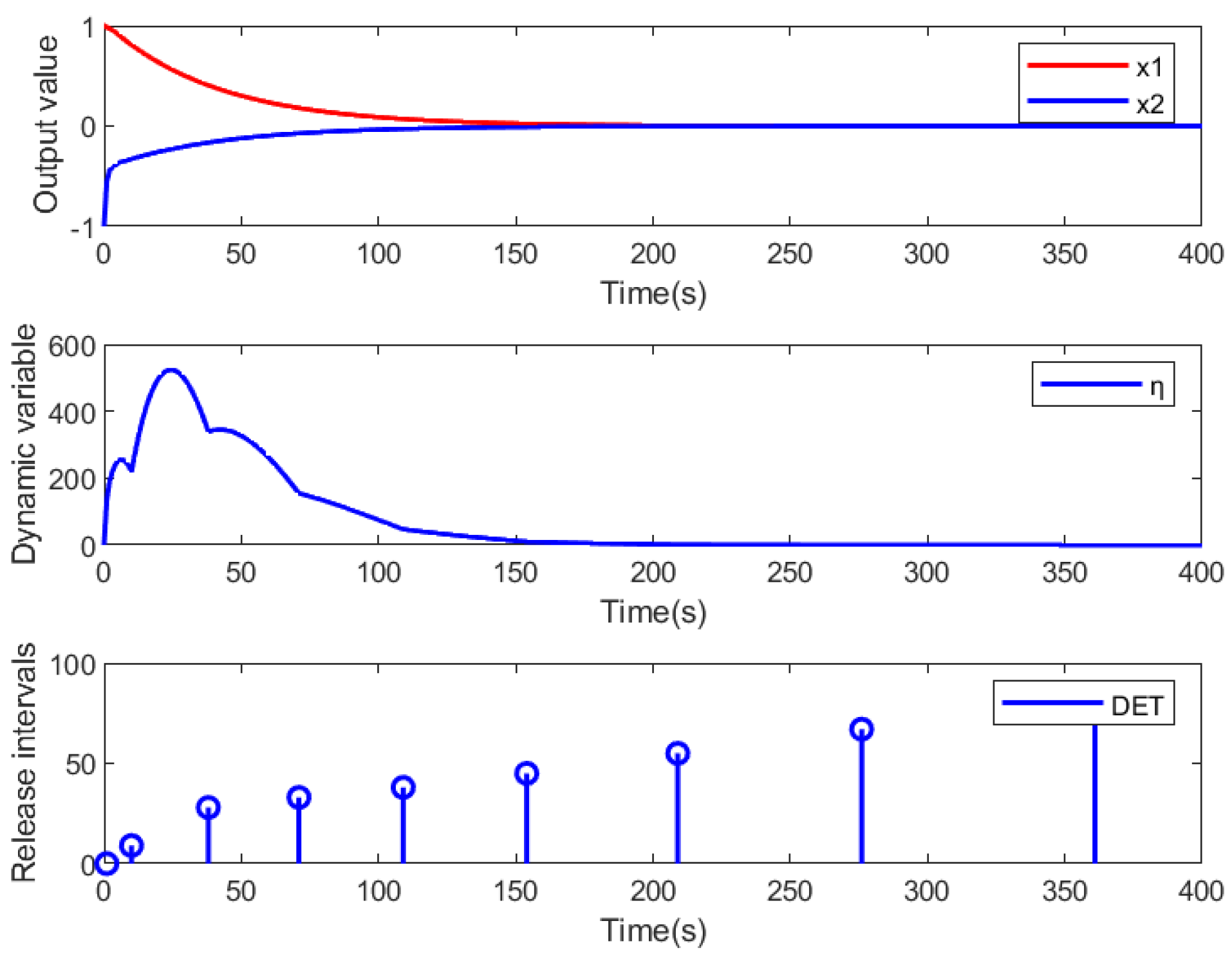
Set x ( 0 ) = 1 1 T , and then apply the trigger condition of (9) in the system (17), where the variable λ is chosen to be the maximum eigenvalue max( λ s ) of the closed-loop systems. The first part of Figure 1 shows that the system is stable, which implies the effectiveness of the controller design method. The second and third parts in Figure 1 illustrate that the event-triggering scheme and parameter design are feasible, and the dynamic variable η 0 .

4.2. Numerical Verify for Results of Unknown Time-Delay System

In this part, the time delay is assumed to be unknown, and it satisfies that τ k 0 , h . The unknown time-delay discrete systems are as follows:
x ( k + 1 ) = A 0 B 0 A 1 x ( k ) u ( k ) x ( t τ k ) .
Data can be obtained as ( U , X ) . Setting h to 8 . Other conditions are consistent with the system described above. By Theorem 2, one obtains W 1 R i × 2 and W 2 R i × 2 , and find the state feedback as follows:
K = U W 1 ( X W 1 ) 1 = 12.2 62.8 .
As shown in Figure 2, the states of the discrete time-delay system is stable, which implies that the proposed method is effective.
Further, it is discussed in what cases these two methods should be carried out to handle discrete time-delay systems. Firstly, in Figure 3, we set τ = 30 , then both methods can control the system. But for higher time delay, the performance of Theorem 1 is not very good. It is clear from Table 2 that the time required for Theorem 1 is much higher than that for Theorem 2. When the time delay increases, the amount of computation increases exponentially and greatly. The amount of computation is often very high, and the requirements are not conducive to our LMI solver obtaining the results; thus, we can use Theorem 2 for a higher time-delay system shown in Figure 4. From the figure, Theorem 2 can also stabilize the system.

4.3. Dynamic Event-Triggering Parameters

When λ = 0.97 and 1 θ = 0.03 , the controller performance is shown in Figure 1. Compared with Figure 2, the event-triggering moments are mainly concentrated on the transient process of the system. Table 3 shows that when λ is chosen as the maximum eigenvalue of the closed-loop system, and 1 θ is chosen to be small. Then, the number of event-triggering scheme is smaller at 9. Therefore, this parameter selection has a better effect on reducing the number of triggering times.
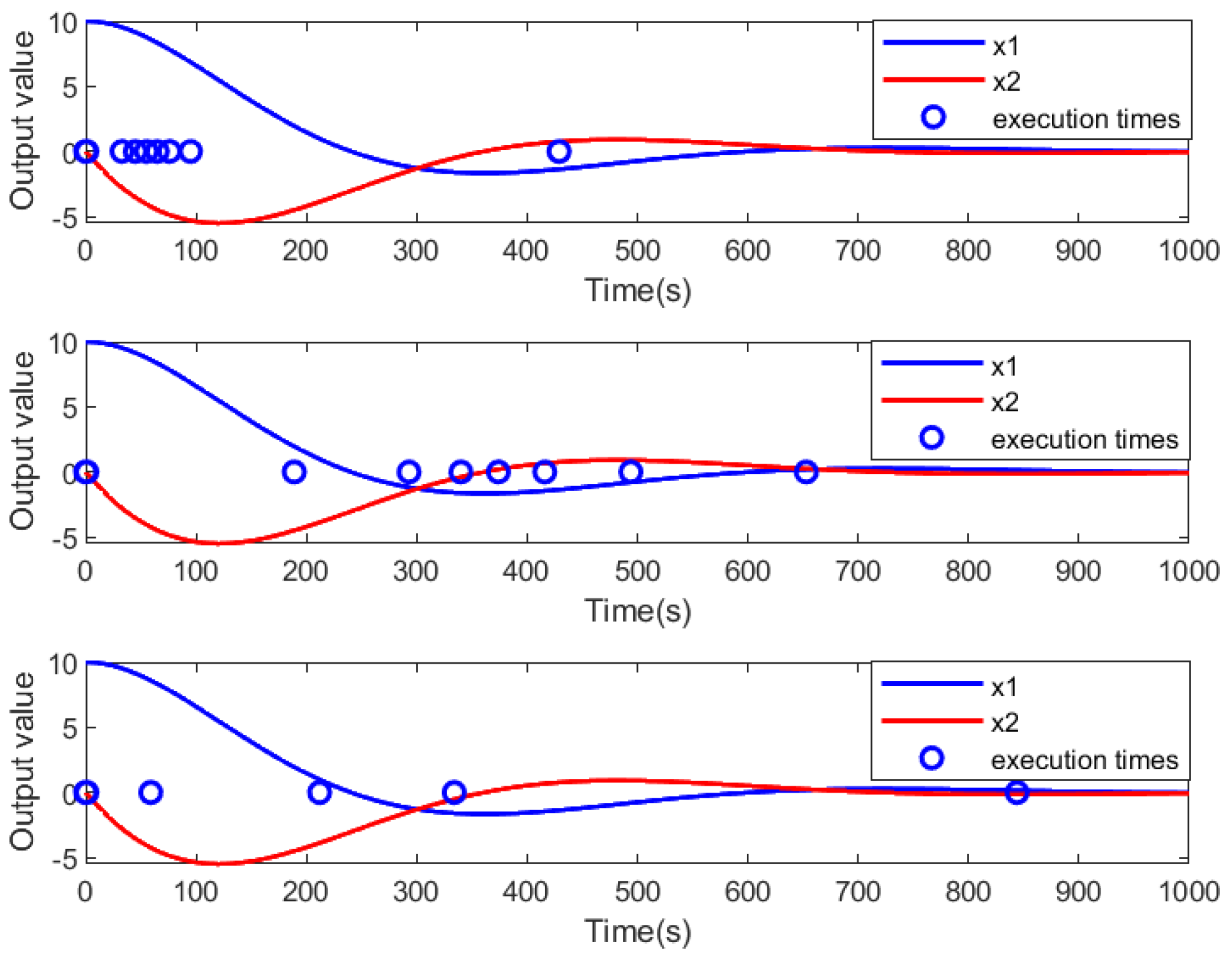
Next, we compare the event-triggering schemes in [17,22]. In Figure 5, the first figure shows the event-triggering scheme method in [17], the second figure shows the event-triggering scheme method in [22], and the third figure shows the event-triggering scheme of (9) and Remark 1. It is obvious from the figures that, for the same system, the selection of the event-triggering parameter proposed in this paper allows for a reduction in the number of event occurrences. Compared with the event triggering scheme proposed in [17], the number of triggers is reduced by 38%. Compared with the event triggering scheme proposed in [22], the number of triggers is reduced by 25%, greatly saving communication and computing resources.

5. Conclusions

This paper proposes a data-driven event-triggered control scheme for time-delay discrete systems, achieving significant progress. In terms of performance improvement, the designed event-triggered mechanism significantly saves communication resources through dynamic threshold optimization. Two cases are discussed: known and unknown time-delay systems, with the improved model method and delay upper-bound method presented. Then, combining the event-triggered scheme, a controller for data-driven systems in discrete time is designed. Experimental validation demonstrates that the scheme effectively optimizes communication resources while ensuring system stability, providing a new solution for intelligent control of time-delay systems. Future research can explore the following directions: developing lightweight algorithms to enhance real-time performance and constructing hybrid triggering mechanisms to enhance environmental adaptability.

Author Contributions

Y.G.: Writing and organization, Writing—review and editing. Z.L.: Model design, Supervision, Software, Formal analysis, Method design. Y.W.: Investigation, Writing—review and editing. All authors have read and agreed to the published version of the manuscript.

Funding

This paper is funded by Intelligent networked Robotic Research Center (Grant No. 602531004PQ) and Guangdong Provincial Department of Education research project (Grant No. 2023ZDZX3077).

Institutional Review Board Statement

Not applicable.

Informed Consent Statement

Not applicable.

Data Availability Statement

The original contributions presented in this study are included in the article. Further inquiries can be directed to the corresponding author.

Conflicts of Interest

The authors declare no conflicts of interest.

References

  1. Van Overschee, P.; De Moor, B. Subspace Identification for Linear Systems: Theory, Implementation, Applications; Springer Science & Business Media: Berlin/Heidelberg, Germany, 1996. [Google Scholar]
  2. Ziegler, J.G.; Nichols, N.B. Optimum settings for automatic controllers. Trans. Am. Soc. Mech. Eng. 1942, 64, 759–765. [Google Scholar] [CrossRef]
  3. Willems, J.C.; Rapisarda, P.; Markovsky, I.; De Moor, B.L. A note on persistency of excitation. Syst. Control Lett. 2005, 54, 325–329. [Google Scholar] [CrossRef]
  4. Markovsky, I.; Rapisarda, P. Data-driven simulation and control. Int. J. Control 2008, 81, 1946–1959. [Google Scholar] [CrossRef]
  5. Park, U.S.; Ikeda, M. Stability analysis and control design of lti discrete-time systems by the direct use of time series data. Automatica 2009, 45, 1265–1271. [Google Scholar] [CrossRef]
  6. Maupong, T.M.; Rapisarda, P. Data-driven control: A behavioral approach. Syst. Control Lett. 2017, 101, 37–43. [Google Scholar] [CrossRef]
  7. Safonov, M.G.; Tsao, T.-C. The unfalsified control concept: A direct path from experiment to controller. In Feedback Control, Nonlinear Systems, and Complexity; Springer: Berlin/Heidelberg, Germany, 1995; pp. 196–214. [Google Scholar]
  8. Hjalmarsson, H.; Gevers, M.; Gunnarsson, S.; Lequin, O. Iterative feedback tuning: Theory and applications. IEEE Control Syst. Mag. 1998, 18, 26–41. [Google Scholar]
  9. Shangtai, H.Z.J. Data-driven model-free adaptive control for a class of mimo nonlinear discrete-time systems. IEEE Trans. Neural Netw. 2011, 22, 2173–2188. [Google Scholar]
  10. Wu, A.-G.; Meng, Y. Data-driven adaptive optimal control for discrete-time linear time-invariant systems. Int. J. Syst. Sci. 2024, 55, 3069–3082. [Google Scholar] [CrossRef]
  11. Vamvoudakis, K.G.; Lewis, F.L. Online actor–critic algorithm to solve the continuous-time infinite horizon optimal control problem. Automatica 2010, 46, 878–888. [Google Scholar] [CrossRef]
  12. Jiang, Y.; Jiang, Z.-P. Computational adaptive optimal control for continuous-time linear systems with completely unknown dynamics. Automatica 2012, 48, 2699–2704. [Google Scholar] [CrossRef]
  13. Salvador, J.R.; de la Peña, D.M.; Alamo, T.; Bemporad, A. Data-based predictive control via direct weight optimization. IFAC-PapersOnLine 2018, 51, 356–361. [Google Scholar] [CrossRef]
  14. Li, Z.; Liu, K.; Wang, X.; Yuan, X.; Wang, Y. Efficient data-driven event-triggered predictive control for cyber-physical systems. J. Control Decis. 2024, 1–10. [Google Scholar] [CrossRef]
  15. Dai, T.; Sznaier, M. A moments based approach to designing mimo data driven controllers for switched systems. In Proceedings of the 2018 IEEE Conference on Decision and Control (CDC), Miami, FL, USA, 17–19 December 2018; IEEE: Piscataway, NJ, USA, 2018; pp. 5652–5657. [Google Scholar]
  16. Tabuada, P. Event-triggered real-time scheduling of stabilizing control tasks. IEEE Trans. Autom. Control 2007, 52, 1680–1685. [Google Scholar] [CrossRef]
  17. Girard, A. Dynamic triggering mechanisms for event-triggered control. IEEE Trans. Autom. Control 2014, 60, 1992–1997. [Google Scholar] [CrossRef]
  18. Yi, X.; Liu, K.; Dimarogonas, D.V.; Johansson, K.H. Dynamic event-triggered and self-triggered control for multi-agent systems. IEEE Trans. Autom. Control 2018, 64, 3300–3307. [Google Scholar] [CrossRef]
  19. Zhang, R.; Liu, H.; Liu, Y.; Tan, H. Dynamic event-triggered state estimation for discrete-time delayed switched neural networks with constrained bit rate. Syst. Sci. Control. Eng. 2024, 12, 2334304. [Google Scholar] [CrossRef]
  20. Li, Q.; Shen, B.; Wang, Z.; Huang, T.; Luo, J. Synchronization control for a class of discrete time-delay complex dynamical networks: A dynamic event-triggered approach. IEEE Trans. Cybern. 2018, 49, 1979–1986. [Google Scholar] [CrossRef] [PubMed]
  21. Wu, W.; Yan, H.; Wang, Y.; Li, Z.; Wang, M. Fixed time cluster consensus for nonlinear multiagent systems by double dynamic event-triggered mechanisms. Int. J. Syst. Sci. 2024, 55, 3322–3336. [Google Scholar] [CrossRef]
  22. Wang, X.; Berberich, J.; Sun, J.; Wang, G.; Allgöwer, F.; Chen, J. Model-based and data-driven control of event-and self-triggered discrete-time linear systems. IEEE Trans. Cybern. 2023, 53, 6066–6079. [Google Scholar] [CrossRef] [PubMed]
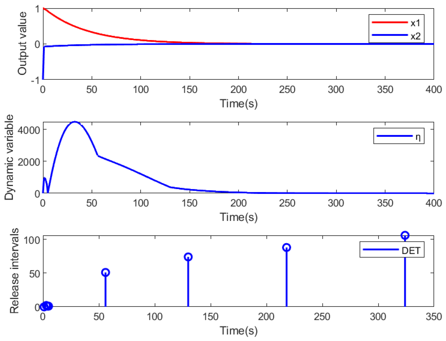
Figure 1. Data−driven (19) under system (17), the trajectory of the dynamic variable η , and the moment of event-triggering times.
Information 16 00893 g001
Figure 2. Data−driven (4) under system (1), the trajectory of the dynamic variable η , and the moment of event-triggering times.
Information 16 00893 g002
Figure 3. The system state of the controller designed by Theorems 1 and 2 when the time delay is 30.
Information 16 00893 g003
Figure 4. The system state and event−triggering moment of the controller are designed according to Theorem 2 when the time delay is 60.
Information 16 00893 g004
Figure 5. The above simulation presents a comparative analysis of event−triggering mechanisms and corresponding system states among [17,22], and our approach in the identical discrete system setting.
Information 16 00893 g005
Table 1. EV Parameters.
SymbolParameters
τ Time delay
α Threshold Parameter
λ Decay Factor
θ Weighting Parameter
X a u g Augmented System Matrix
U a u g Augmented Input Matrix
P ^ , R ^ , Q ^ and S ^ Square Matrix
W 1 Pseudoinverse matrix of X
W 2 Pseudoinverse matrix of X +
Table 2. Calculation time for the lifting model method and the delayed upper bound method.
Time Delay ( τ )25101520
Theorem 10.30 s7.25 s110.95 s568.33 s1965.89 s
Theorem 2 (h = 50)0.06 s0.07 s0.07 s0.07 s0.07 s
Table 3. The number of times an event-triggering scheme occurs when the event-triggering scheme parameters 1 θ and λ are different in system (1).
Parametric 1 θ = 0.001 1 θ = 0.03 1 θ = 0.2 1 θ = 0.4 1 θ = 0.6
λ = 0.97139111212
λ = 0.81919171616
λ = 0.61919181818
λ = 0.41919191919
Disclaimer/Publisher’s Note: The statements, opinions and data contained in all publications are solely those of the individual author(s) and contributor(s) and not of MDPI and/or the editor(s). MDPI and/or the editor(s) disclaim responsibility for any injury to people or property resulting from any ideas, methods, instructions or products referred to in the content.