Article

An Intelligent Algorithm for the Optimal Deployment of Water Network Monitoring Sensors Based on Automatic Labelling and Graph Neural Network

1
Hainan Provincial Key Laboratory of Low-Altitude Intelligent Sensing and Information Processing, School of Information and Communication Engineering, Hainan University, Haikou 570228, China
2
Guangdong Water Co., Ltd., Shenzhen 518021, China
*
Authors to whom correspondence should be addressed.
Information 2025, 16(10), 837; https://doi.org/10.3390/info16100837
Submission received: 7 August 2025 / Revised: 10 September 2025 / Accepted: 25 September 2025 / Published: 27 September 2025

Abstract

In order to enhance leakage detection accuracy in water distribution networks (WDNs) while reducing sensor deployment costs, an intelligent algorithm for the optimal deployment of water network monitoring sensors based on the automatic labelling and graph neural network (ALGN) was proposed for the optimal deployment of WDN monitoring sensors. The research aims to develop a data-driven, topology-aware sensor deployment strategy that achieves high leakage detection performance with minimal hardware requirements. The methodology consisted of three main steps: first, the dung beetle optimization algorithm (DBO) was employed to automatically determine optimal parameters for the DBSCAN clustering algorithm, which generated initial cluster labels; second, a customized graph neural network architecture was used to perform topology-aware node clustering, integrating network structure information; finally, optimal pressure sensor locations were selected based on minimum distance criteria within identified clusters. The key innovation lies in the integration of metaheuristic optimization with graph-based learning to fully automate the sensor placement process while explicitly incorporating the hydraulic network topology. The proposed approach was validated on real-world WDN infrastructure, demonstrating superior performance with 93% node coverage and 99.77% leakage detection accuracy, surpassing state-of-the-art methods by 2% and 0.7%, respectively. These results indicate that the ALGN framework provides municipal water utilities with a robust, automated solution for designing efficient pressure monitoring systems that balance detection performance with implementation cost.

1. Introduction

Water distribution networks (WDNs) are critical urban infrastructure systems, yet they increasingly face structural deterioration caused by aging pipelines and environmental factors [1]. Globally, annual water losses from leaks are estimated at over 1 billion cubic meters—sufficient to supply 10 million people [2]. Pipe failures also risk introducing harmful contaminants that threaten public health [3]. These challenges have driven advancements in monitoring technologies, particularly through integration with supervisory control and data acquisition (SCADA) systems, enabling a transition from periodic inspections to continuous data-driven surveillance [4]. The literature suggests that data-driven leak detection methods for WDN will be the future research trend, and effective leak detection relies on strategically positioned sensors that capture hydraulic anomalies across the network [5]. Traditional methods include those based on hydraulic sensitivity analysis, redundant design, and pipeline roughness calibration. For instance, Ferreira et al. [6] employed a pressure-sensitive matrix to search for the optimal sensor position for the calibration problem of pipeline roughness coefficients. Di Nardo et al. analyzed the redundancy characteristics of the water supply network [7]. Weber et al. designed methods for calibrating pipe roughness and placing sensors [8]. The selection of optimal sensor locations must balance detection sensitivity with infrastructure coverage, particularly given budgetary constraints in municipal water management. Current sensor deployment strategies generally fall into two categories: intelligent algorithm-based and machine learning-based methods.
Intelligent algorithm-based methods leverage advanced optimization techniques to efficiently determine sensor placements by rapidly evaluating objective functions. For instance, Meier et al. were among the first to introduce genetic algorithms for sensor placement, transforming the problem into a search optimization task [9]. Xiao Zhou et al. employed a pressure sensitivity matrix as the optimization objective, utilizing genetic algorithms to refine the number and locations of pressure monitoring points [10]. Wang T et al. proposed a hydraulic influence correction method, which took pressure monitoring coverage index and average maximum dimensionless quantity as optimization objectives, and, based on the Non-dominated Sorting Genetic Algorithm (NSGA-||), realized the arrangement of pressure monitoring points in WDN [11]. Cheng et al. further advanced this approach by optimizing an objective function specifically tailored for leak detection, achieving notable improvements through genetic algorithms [12]. Fei et al. conducted a comparative analysis between the bat algorithm and particle swarm optimization, demonstrating the superior performance of the bat algorithm in optimizing pressure sensor placement within WDNs [13].
Machine learning-based sensor placement optimization methods utilized machine learning and deep learning techniques to first cluster nodes based on their intrinsic features and then determine the most suitable node within each cluster for sensor deployment. Li Cheng et al. formulated the pressure-leak sensitivity matrix by incorporating the characteristics of both nodes and pipes, then applying K-means clustering to identify cluster centers as optimal pressure monitoring points [14]. Fei et al. utilized fuzzy C-means and moth flame optimization methods to optimize underwater sensor networks [15]. Romero-Ben et al. proposed a model-free method for placing pressure sensors in WDNs [16]. These methods, based on intelligent algorithms and machine learning algorithms, have all achieved very good results. The results demonstrated that the deployed sensors were evenly distributed across the network, ensuring comprehensive coverage. However, although these methods have achieved commendable results, several challenges remain unresolved. As an interconnected and complex system, WDN exhibits not only the hydraulic characteristics of individual nodes but also the connectivity and topological structure among nodes [17]. Methods that consider only hydraulic features without accounting for the topological features may reduce the effectiveness of pressure sensor monitoring.
In recent years, the success of graph neural networks has sparked considerable interest in their potential within engineering. Among them, Graph Convolutional Networks (GCNs) were introduced by Thomas N. Kipf and Max Welling in 2017 [18]. GCNs can handle complex relational data by learning node representations based on graph connectivity. Due to the unique advantages of graph neural networks, applying GCNs to the optimization problem of pressure monitoring points in WDNs can effectively solve the problems that intelligent optimization algorithms and machine learning methods cannot handle, that is, not considering the topological structure of the WDN. Peng et al. proposed a sensor placement method for pressure monitoring that leverages the Structural Deep Clustering Network (SDCN) to learn both the network topology and hydraulic characteristics, thereby clustering nodes effectively [19]. Jun Li et al. developed an Embedding Graph Auto-Encoder (EGAE)-based approach that utilizes an Embedding Graph Auto-Encoder to cluster nodes and determine optimal sensor locations [20]. Zhang et al. proposed a sensor layout method for WDNs based on Graph Convolutional Neural Networks [21]. Zhou et al. utilized the graph Fourier transform to process graph signals and achieve the optimal sensor layout [22]. Giacomo et al. summarized the current methods for modeling and optimizing WDNs using graph neural networks [23]. These methods have achieved excellent clustering results. However, they all require manual input of parameters, and the parameters have a significant impact on the clustering effect.
To solve the above problems and improve the accuracy of clustering, this paper proposed an intelligent algorithm for the optimal deployment of water network monitoring sensors based on automatic labelling and adaptive weight distribution. The parameters of the DBSCAN algorithm were optimized using the DBO algorithm to automatically determine the number of clusters and the initial labels of the clusters. The method proposed in this paper can adaptively allocate parameters and weights, and simultaneously consider the connectivity between nodes and the hydraulic characteristics of each node when clustering nodes. Our method only requires the input of the pipe network topology structure and the node pressure sequence, and it can adaptively obtain the optimal number of WDN node clusters and the optimal clustering results, achieving a fully automatic layout of pressure monitoring points.

2. Methodology

The technical route of the proposed method, based on the automatic labelling and graph neural network (ALGN), is shown in Figure 1. This method can be divided into three steps: the pre-training stage, the clustering stage, and the monitoring point layout stage. In the pre-training stage, two tasks are carried out at the same time: (1) Construct the feature matrix and cluster the feature matrix by the density-based noise application spatial clustering (DBSCAN) algorithm optimized by the dung beetle optimization algorithm (DBO) to obtain the initial label of each node. The dung beetle optimizer (DBO) algorithm finds the optimal values for the two key DBSCAN parameters: the neighborhood radius (EPS) and the minimum number of points (MINPTS). It achieves this by searching for the parameter pair that maximizes a clustering performance metric. The number of clusters is not pre-defined by the user but is automatically determined by the combined DBO-DBSCAN process. The DBSCAN algorithm then uses these optimized parameters to form clusters based on data density, with the resulting number of clusters being a natural outcome of this density-based partitioning. The specific steps of the DBO-DBSCAN algorithm are introduced in Section 2.1.1. (2) Input node features into the auto-encoder to obtain higher-order features. In the clustering stage, the adjacency matrix and node features are input into the initial layer of the Graph Convolutional Network (GCN), and the higher-order features obtained by the auto-encoder are input into the GCN layer by layer. The adjacency matrix contains the connectivity relationships between nodes in the water system. The self-attention module is used to assign the weight of the higher-order feature and the inter-layer feature of GCN, and a more representative feature is obtained. Then, the network is trained by using a dual self-supervision mechanism and an auto-encoder loss to construct the loss function, and finally, the clustering result of each node is obtained. Steps are detailed in Section 2.2. In the monitoring point layout stage, the interdomain distance between each node is calculated according to the clustering results of nodes, and the node with the smallest interdomain distance is selected as the pressure monitoring point. These three steps are described in detail in Section 2.1, Section 2.2 and Section 2.3.

2.1. Pre-Training

2.1.1. The Improved DBSCAN Algorithm

GCN is a semi-supervised task; each node is initially unlabeled. Therefore, it is necessary to initialize the label for each node in the pipe network. As a density-based clustering algorithm, the advantage of DBSCAN is that it can adaptively determine the number of clusters based on the characteristics and density of nodes [24]. The two key hyperparameters in DBSCAN are the minimum radius EPS of clustering and the minimum number of MINPST points, where EPS represents the domain radius of the sampling points, and MINPST represents the minimum number of points in each cluster. Based on the above concepts, the sample points can be divided into core points, boundary points, and noise points. Among them, the core point is the core of the cluster, the boundary point is the point within the class adjacent to a certain core point, and the noise point is the outlier. The basic flow of the DBSCAN algorithm is as follows:
  • Select any point X in the sample.
  • Take this point as the center and EPS as the radius. If the number of sample points within the range is greater than or equal to MINPST, specify this point as the core point; otherwise, it is a non-core point.
  • Start with adjacent samples at point X and repeat step 2 until all samples in this dataset are traversed. Finally, the clustering results, including core points, noise points, and non-core points, are obtained.
The DBSCAN algorithm requires manual input of parameters EPS and MINPTS, and the selection of these two parameters directly affects the accuracy of the clustering. When EPS is determined and MINPTS increases, the definition of the core point will become stricter, and a point needs more neighbors to become a core point. Some points that could have been classified as a category will no longer meet the conditions and become noise points. This leads to an increase in noise points and a decrease in the number of clusters. This eventually led to a decrease in the number of sensors. A reduction in the number of sensors deployed will lead to poor monitoring performance of the system. When EPS is determined and MINPTS decreases, many noise points will become points within the class. This ultimately leads to an increase in the number of clusters and sensors. When MINPTS is determined and EPS decreases, many points will become noise points. However, as the number of points in each class decreases, the number of clusters will also increase. When MINPTS is determined and EPS increases, it will lead to a large number of core points, causing the number of clusters to increase. Eventually, this will result in an increase in the number of sensors. Once the number of sensors reaches a certain level and is further increased, it will lead to sensor redundancy and a waste of resources. Therefore, the appropriate method needs to be selected to determine the optimal EPS and MINPTS. In this paper, the DBO algorithm was introduced [25] to improve DBSCAN. Its basic principles are as follows:
First of all, the fitness function is defined as follows:
f i t n e s s = 1 S
where S is the value within [ 1 , 1 ] , which is called the average silhouette coefficient of the cluster. And with the growth of S, the performance of clustering is also increasing. Suppose the nodes are divided into o clusters, then the value of S is calculated according to the following formula:
S = 1 O i = 1 O S ( p i )
S ( P i ) = b ( p i ) a ( p i ) max { b ( p i ) , a ( p i ) }
where S ( p i ) represents the silhouette coefficient of each cluster. The role of a ( p i ) is to quantify the cohesion of the cluster, and the a ( p i ) value is obtained from p i and the average distance of the other samples. b ( p i ) represents the minimum average distance from p i to all neighboring clusters, which is used to quantify the degree of separation between clusters.
During the exploration stage, we classified dung beetles into ball-rolling dung beetles, breeding dung beetles, foraging dung beetles, and stealing dung beetles based on their nature and lifestyle. Different populations have different lifestyles, but they all keep moving towards food points (i.e., the optimal points) under the influence of their own and external factors. The positions of the ball-rolling dung beetle are updated as follows:
x i ( t + 1 ) = x i ( t ) + α × k × x i ( t 1 ) + b × Δ x
Δ x = | x i ( t ) x w |
where t represents the current iteration number, x i ( t ) represents the position of the i-th dung beetle at the t iteration, k ( 0 , 2 ] is a constant representing the deflection coefficient, b ( 0 , 1 ) , α is the natural coefficient of 1 or −1, x w is the global worst position, and Δ x represents the change in light intensity.
When the ball dung beetle encounters an obstacle, it will randomly rotate to regain its direction. Therefore, the dung beetle updates its position as follows:
x i ( t + 1 ) = x i ( t ) + tan ( θ ) | x i ( t ) x i ( t 1 ) |
where θ is the deflection angle belonging to [ 0 , π ] .
In order to provide a safe environment for the offspring, the breeding area of dung beetles is defined as follows:
L b * = max ( X * × ( 1 R ) , L b )
U b * = min ( X * × ( 1 R ) , U b )
where X * represents the current local optimal position, L b * and U b * represent the upper and lower bounds of spawning, R = 1 t / T max , T max denotes the maximum number of iterations, and L b and U b represent the upper and lower bounds set by the optimization problem. After determining the egg-laying area, the reproductive dung beetles will lay eggs in this area. The position of the egg balls also changes dynamically with the number of iterations and is defined as follows:
B i ( t + 1 ) = X * + b 1 × ( B i ( t ) L b * ) + b 2 × ( B i ( t ) U b * )
where B i ( t ) is the position of the i egg at the t iteration, b 1 and b 2 are two random vectors of size 1 × D , and D is the dimension of the optimization problem.
The foraging beetles forage within the boundary, which changes dynamically with the number of iterations:
L b b = max ( X b × ( 1 R ) , L b )
U b b = min ( X b × ( 1 + R ) , U b )
where X b represents the global optimal position and L b b and U b b represent the upper and lower bounds of the foraging boundary, respectively. From this, the position of the foraging dung beetle is obtained:
x i ( t + 1 ) = x i ( t ) + C 1 × ( x i ( t ) L b b ) + C 2 × ( x i ( t ) U b b )
where C 1 is a normal random number and C 2 is a random number within ( 0 , 1 ) .
The stealing beetles’ position update formula is as follows:
x i ( t + 1 ) = X b + S × g × | x i ( t ) X * | + | x i ( t ) X b |
where g is a normally distributed random vector of size 1 × D and S is a random constant.
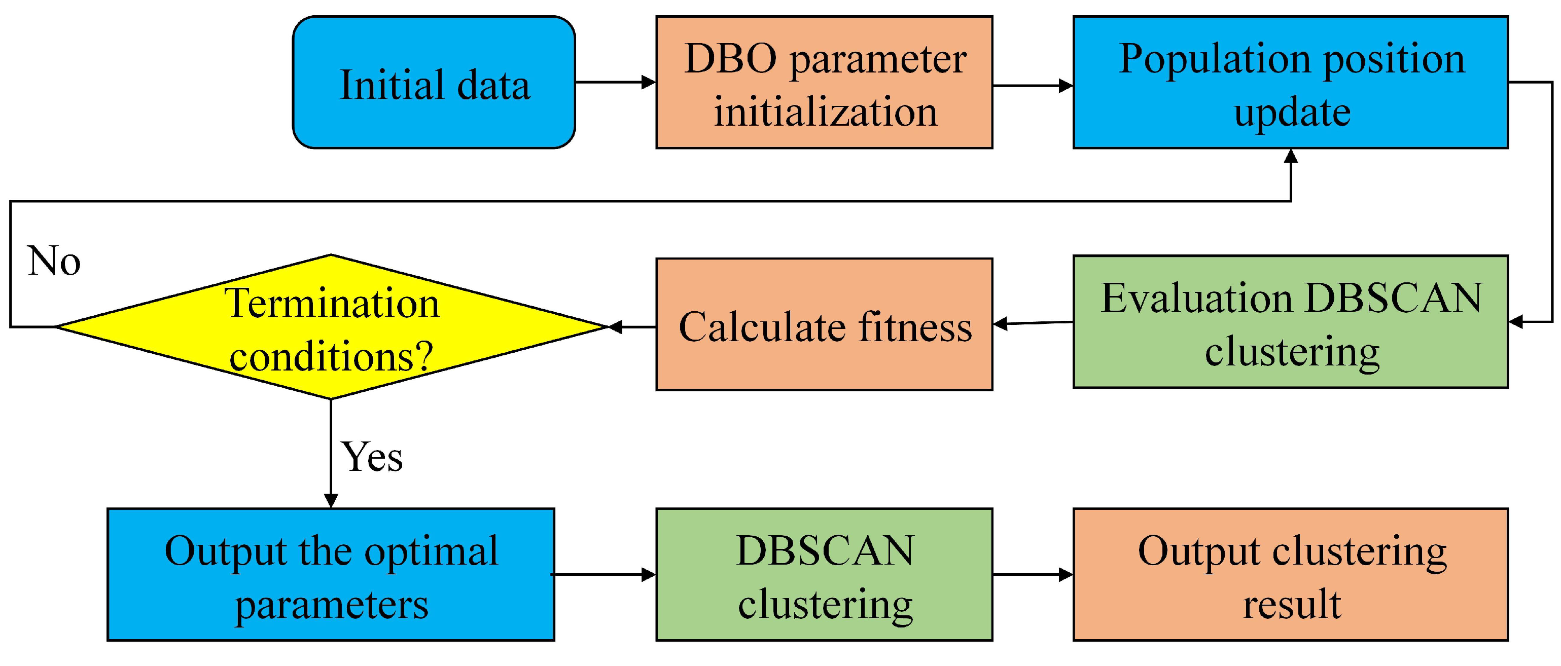
In the DBO algorithm, during the exploration stage, different types of dung beetles influence each other and gradually update their positions according to their respective position update formulas, taking into account both global search and local utilization. Figure 2 presents the flow block diagram of the DBO-DBSCAN algorithm. This improved algorithm first sets the contour coefficient of DBSCAN as the optimization objective of DBO, then enables the DBO algorithm simulating the dung beetle population to search and iterate in the parameter space (EPS, MINPTS), and finally outputs the parameter combination that optimizes the performance of DBSCAN, thereby achieving the complete automation and optimization of the clustering process.
In the process of data initial clustering, the node feature matrix is constructed as the input data for the DBSCAN module initialization. The feature matrix is constructed by using nodal influence degree in hydraulics and standard deviation in statistics. Among them, the construction method of the node feature matrix is as follows:
  • Obtain the pressure P of the WDN under normal operating conditions.
  • Change the node water requirements one by one to obtain the node water pressure Q = { Q 1 , Q 2 , , Q N } of N nodes.
  • Calculate the node pressure difference:
    R i = P Q i
  • Calculate the impact level of each node:
    S i = 1 m n i = 1 m b = 1 n ( R tb - d y i ) 2
    where S i represents the influence degree of the node.
  • Calculate the standard deviation of each node:
    σ i = 1 m i = 1 m P i i 1 m ( P 1 i + P 2 i + + P m i ) 2
    where σ i represents the standard deviation of nodes.
  • Construct the node eigenmatrix V i = [ x i , y i , S i , σ i ] T of the i node, indicating that the data are connected; x and y denote the coordinates of the node.

2.1.2. Auto-Encoder Module

It was very important for the GCN module to obtain an effective representation of the data. Auto-encoders were used to learn the underlying characteristics of the data [26]. It consists of an encoder and a decoder. The encoder is a fully connected neural network. For the L layer of the encoder, its data representation H en L is as follows:
H en L = sig mod ( W en L H en L 1 + b en L )
where H en L represents the data representation of the encoder layer L, sigmod represents the sigmod activation function, and W en L and b en L represent the weight and bias of the encoder layer.
The decoder and encoder have the same structure, and the L-layer data of the decoder is represented as:
H de L = sigmod ( W de L H de L 1 + b de L )
W de L and b de L represents the weight and bias of the decoder layer.
The initial input data X is finally reconstructed after the encoder and decoder. The objective function of the auto-encoder is:
L A E = 1 2 N i = 1 N X X ^ F 2

2.2. Clustering

2.2.1. GCN Module

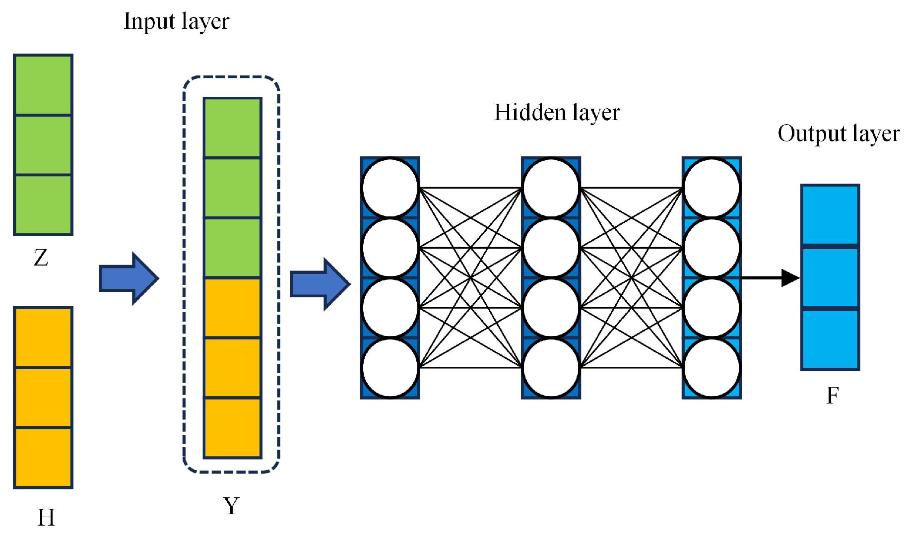
As shown in Figure 3, input the adjacency matrix A of the WDN, node features X, and the node feature representation H of the auto-encoder into the GCN module, and the GCN learns these representations through hierarchical propagation.
The adjacency matrix A represents the connectivity between each node in the pipe network. A is an n × n size matrix, where n represents the number of nodes, and is 1 at two connected points and 0 at two unconnected points. After the GCN learns all the representations, it can accommodate different information at the same time, that is, the data itself and the relationships between them. For layer L of GCN, the calculation formula for its data representation Z L is as follows:
Z L = sigmod D ˜ 1 2 A ˜ D ˜ 1 2 F L 1 W L 1
where A ˜ = A + I , I represents the identity matrix and D ˜ represents the degree matrix, which represents the number of nodes directly connected to each node, multiplying D ˜ 1 2 around A ˜ to prevent magnitude differences in feature propagation. For example, a high-number node may aggregate features of many neighbors; while the features of a low-number node may be diluted, it needs to be normalized. F L 1 represents the output of the self-attention module, which is described in detail below.
In particular, for the first layer of GCN, the hierarchical propagation formula is:
Z 1 = sigmod D ˜ 1 2 A ˜ D ˜ 1 2 X W 1
For the last layer of GCN, the softmax function was used to classify:
Z = softmax D ˜ 1 2 A ˜ D ˜ 1 2 F L W L
The final result z i j Z represents the probability that the sample i belongs to the cluster center j.

2.2.2. Self-Attention Module

The hidden features of the data were extracted by the auto-encoder. The feature Z was extracted by the GCN. Both data representations extract node features, but are essentially different representations. A self-attention module was designed to better integrate these two data representations [27]. The self-attention module allocated attention to the representations learned by the GCN module and the auto-encoder module, and integrates them layer by layer. Finally, the data representation contains both node characteristics and pipe network topology, and a more representative data representation is constructed.
Figure 4 shows the structure of the self-attention module. It consisted of two fully connected layers and a softmax layer. The first hidden layer contains 64 neurons, and the second hidden layer contains 64 neurons. The Softmax layer converts the original values output by the neural network into a probability distribution, making the sum of all output values 1. Its output value represents the probability that the input sample belongs to each category, thereby solving the final decision of multi-classification problems. In layer L, auto-encoder data are represented by H L and GCN data are represented by Z L . We carry out the following:
Y L = [ Z L , H L ]
For constructed features Y L , we identify their importance through the constructed self-attention module:
a = f ( Y L )
c = softmax sigmod ( a ) / τ
W = mean ( c , dim = 0 )
where f ( · ) represents the fully connected layer of the structure and τ represents the calibration factor, W = [ W Z , W H ] .
Therefore, the output of the L level of the self-attention module is:
F L = W Z Z L + W H H L

2.2.3. Dual Self-Monitoring Module

The auto-encoder module, GCN module, and self-attention module have been connected. However, the auto-encoders were used for data representation learning and belong to unsupervised learning. The GCN module was used for data adjacency feature learning and belongs to semi-supervised learning. They cannot be used directly for clustering nodes. Therefore, a dual self-supervised module is designed to train these modules from end to end [28].
For the i-th sample and the j-th class, Student’s t-distribution was used to measure the node similarity between the node representation h i and the cluster center μ j , and the Q distribution of the sample representation is obtained:
q i j = 1 + h i μ j 2 v v + 1 2 j 1 + h i μ j 2 v v + 1 2
where h i represents the line i of the encoder data representation H en L and μ j represents the j-th cluster center, which is initialized by the DBSCAN algorithm.
After obtaining the clustering result distribution Q, we wanted to obtain the data representation closer to the cluster center. Therefore, the target distribution P was calculated as follows:
p i j = q i j 2 f j j q i j 2 f j
where f j = i q i j represents soft clustering frequency.
The KL divergence of the target distribution P and Q was calculated. By minimizing the KL divergence, the auto-encoder can help to obtain better data representation. This is a self-monitoring mechanism because the target distribution P is calculated from the distribution Q, which, in turn, monitors the update of the distribution Q.
L P Q = K L ( P Q ) = i j p i j log p i j q i j
The training of the GCN module was determined by the distribution Z and the target distribution P. We complete the training of the GCN module by calculating the KL divergence of Z and P. The target distribution P is calculated by distribution Q, and distribution Q and distribution Z influence each other, jointly affect training, and form mutual supervision.
L P Z = K L ( P Z ) = i j p i j log p i j z i j
Each module fully obtained the characteristics of the data through the above loss function to optimize. Moreover, the learned data contain both node characteristics and the topology structure of the pipe network, and the clustering results are more robust.
By combining the data reconstruction loss in AE L A E , and SSC loss L P Q and L P Z , we obtain the total objective function of the proposed model as
min L = L A E + λ 1 L P Q + λ 2 L P Z
where λ 1 and λ 2 are hyperparameters that balance the importance of various losses.

2.3. Placement of Monitoring Points

After clustering was completed, the WDN was divided into different areas. For nodes in the same region, the correlation distance was used to measure the similarity between each node. The correlation distance is defined as follows:
ρ X Y = C o v ( X , Y ) D ( X ) D ( Y ) = E ( ( X E X ) ( Y E Y ) ) D ( X ) D ( Y )
D X Y = 1 ρ X Y
where D X Y represents the correlation distance and ρ X Y represents the correlation coefficient; the greater the correlation coefficient, the higher the degree of correlation. D ( · ) represents the variance and E ( · ) represents the mean.
The correlation distance of all nodes is calculated by Formula (34). Correlation distance indicates the correlation between nodes to some extent. The node with the smallest correlation distance is selected as the pressure monitoring arrangement point.

2.4. Leakage Identification

During the leakage identification stage, the system first acquires the pressure sensor data deployed at the core nodes of the pipeline network in real time and constructs a pressure spatio-temporal matrix (sensor nodes are listed as time series). After standardization, this matrix is used as input data. Subsequently, the matrix was input into the ResNet-18 deep learning model. The model automatically extracts the deep features of pressure changes through its multi-layer convolutional structure and residual connection and outputs the classification probability. If it is determined to be in a leakage state and the confidence level exceeds the set threshold, a leakage alarm will be triggered so as to achieve rapid and accurate leakage identification.

3. Results and Discussion

In this section, two cases were analyzed to verify the effectiveness of our algorithm (a constructed network and a real network). The algorithm’s data requirements necessitate obtaining the pressure sequences for all nodes in the network. The hydraulic simulations were performed using the Water Network Tool for Resilience (WNTR) package within a Python 3.8 environment [29]. In the experiments, ResNet18 was used as a classifier. The learning rate of the neural networks was set to 0.01 and decreased as the training batch increased. The optimizer used was the Adam optimizer [30].

3.1. Evaluation Indicator

The purpose of arranging water distribution network (WDN) monitoring points is to arrange reasonable pressure monitoring points, to achieve the purpose of comprehensive monitoring of WDN, and to achieve better monitoring of leakage. It is necessary to assess the operational status of the WDN by adopting appropriate evaluation indicators. Different indicators will have different impacts on the supervision and leakage management activities of water supply companies [31]. Therefore, two indicators were used to measure the quality of the pressure monitoring points:
  • Detection range of the monitoring point;
  • Accuracy of leakage monitoring of WDN.
For indicator 1, a tensor diagnosability indicator was proposed to measure the detection range of the monitoring points. This indicator is calculated as follows:
Simulate the pressure data of the WDN under different working conditions σ and different nodes N to obtain a four-dimensional pressure tensor of σ × N × ε × K , where K refers to the length of the time series, which is equal to the simulation duration/time step, and ε refers to the number of monitoring points. For example, for one leak simulation, we obtain a matrix of ε × K .
For the obtained tensor, we perform probability density fitting on all data at the n-th node and k time point, and select the value P n , k for P ( x > P n , k ) = 95 % as the threshold. Values greater than P n , k are regarded as values that can be perceived as leaking and are marked as 1, and values less than P n , k are regarded as values that cannot be perceived as leaking and are marked as 0.
Finally, all the simulated data were analyzed. If there is a data point of 1 in this simulation, we can assume that the leak of size σ created at the node can be detected by the pressure monitoring point that is placed. If all the data in this simulation are 0, then we believe the leak of the size σ created at the node cannot be detected by the pressure monitoring point that is in place. For the result of a certain arrangement, the calculation formula of node coverage is as follows:
θ = D σ N D N
where D σ N indicates the number of leaks that can be detected and D N denotes the total amount of manufactured leakage.
Tensor diagnosability metrics are used to evaluate the quality of sensor layout to see if it can capture sufficient unique information to measure different leaks. For instance, a simple network has two sensors that record pressure data at three different times, forming a 2 × 3 matrix (a second-order tensor). If leaks at two different locations always cause the two sensors to have exactly the same pressure change pattern, it will be very difficult to distinguish between the two leaks. On the contrary, if leakage A causes a small change in one sensor and a large change in another, while leakage B causes a large change in one sensor and a small change in the other, it indicates that the leakage can be well distinguished and the optimal sensor layout has been achieved.
For indicator 2, ResNet18 was used as the leak detection classifier to diagnose the leakage situation of the pipeline network [32], and the accuracy was used to evaluate the pros and cons of the arranged monitoring points (obviously, a higher diagnostic accuracy means better layout).
Different arrangement methods of pressure monitoring points will lead to different arrangement positions of monitoring points, and the time series pressure data will be different. There are also differences in the characteristics of the collected data. Therefore, for the pressure monitoring points arranged by different methods, we trained the ResNet18 network individually using data collected from different monitoring points to ensure the fairness of the experiment.

3.2. Case 1: Simple Net

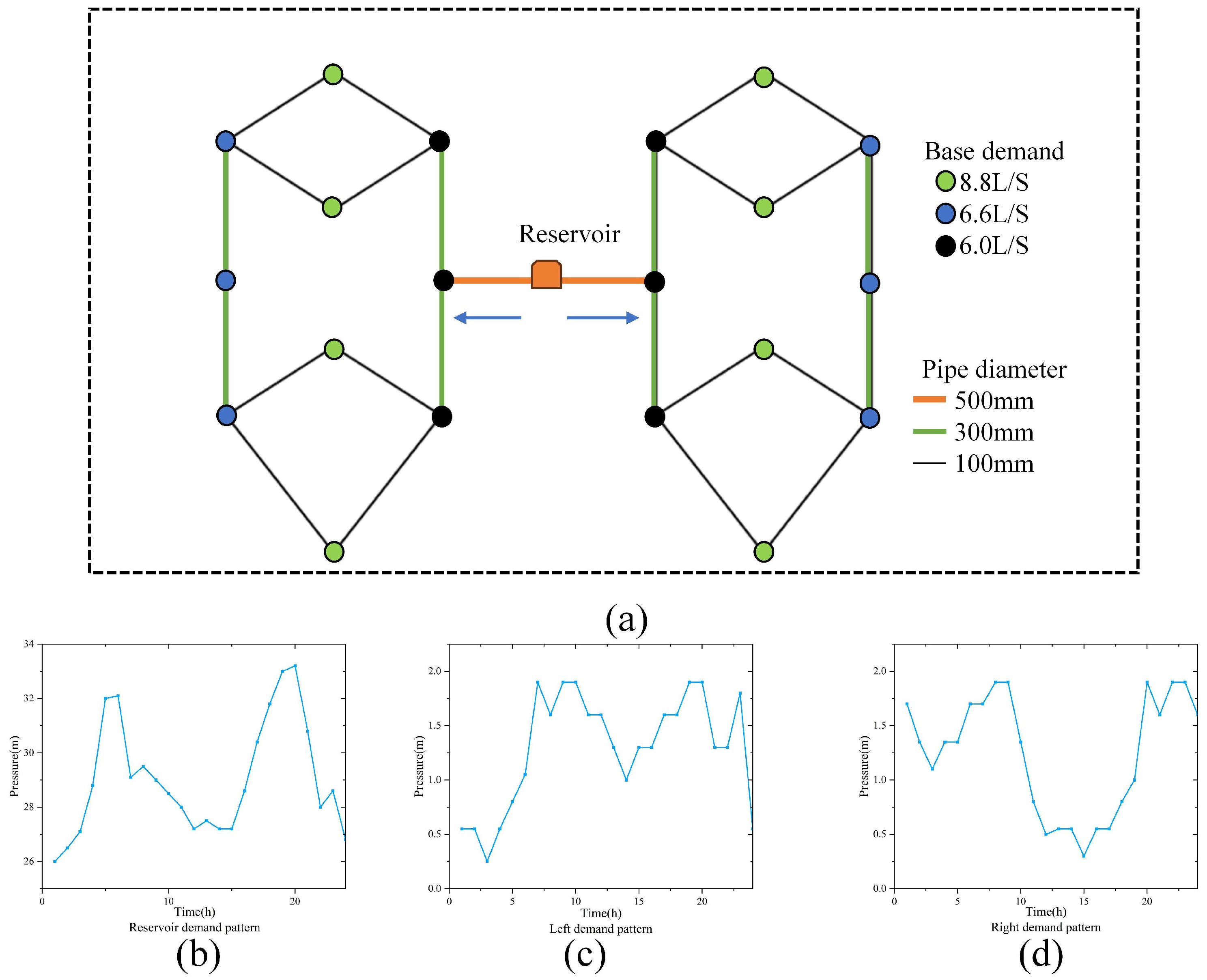
Firstly, a WDN with a special structure was constructed to verify whether the algorithm takes into account both the hydraulic properties and topology of the pipe network. The Simple net consisted of 20 nodes, 26 pipes, and 1 reservoir; the pipe diameter and pipe network structure are shown in Figure 5.
It can be seen from Figure 5 that the Simple net has a left–right symmetric topology, but the left–right hydraulic mode is completely different.
First, a hydraulic simulation of the WDN under normal operating conditions was conducted using the Water Network Tool for Resilience (WNTR, version 1.3.0) software package implementing pressure-driven demand (PDA) modeling. The simulated nodal pressure time series were subsequently input into our spectral clustering algorithm along with the network topology represented as an adjacency matrix. Our proposed method generated the partitioning results shown in Figure 6a, demonstrating that the proposed method successfully categorized network nodes into two distinct clusters. Notably, the clustering result combined both hydraulic dynamic characteristics and topological connectivity considerations, thereby enabling more effective district metered area (DMA) delineation, improved network management efficiency, and resilience enhancement.
Then the DBSCAN algorithm and K-means algorithm were used to cluster the Simple net, and the results are shown in Figure 6b,c. Among them, the DBSCAN method clustering method of WDN nodes selects three characteristic attributes of node coordinates, impact level, and standard deviation of pressure to construct the node feature matrix, and then clusters the node feature matrix using the DBSCAN algorithm. EPANET was used to simulate the pressure conditions of each node in the pipe network when leakage occurred, and the pressure values of all nodes under different leakage conditions were recorded. The pressure difference or change rate between the normal working condition pressure and the leakage working condition pressure is calculated, and a “node-leakage” pressure sensitivity matrix is finally formed as a behavior node and listed as the leakage working condition. This matrix reveals the response pattern of node pressure to leaks at different locations. The K-means method calculates the pressure leakage sensitive matrix of nodes and then clusters the row vectors of the node pressure leakage sensitive matrix by the K-means algorithm.
It can be seen from Figure 6 that the K-means algorithm only considered the hydraulic characteristics of the WDN and divided the Simple net into two categories according to the size of the hydraulic characteristics. The spatial feature matrix constructed by the DBSCAN algorithm considered both the spatial characteristics and hydraulic characteristics of the WDN, and a reasonable clustering result was obtained. Therefore, it is reasonable to use the DBSCAN method cluster label as the pre-training label of the proposed method.
We simulated a randomly sized leak at each node once. Different data were obtained based on the different positions of the sensors arranged by different methods. Finally, the node coverage rates of the four methods are shown in Table 1. It can be seen that due to the different results of clustering, the locations of monitoring points vary, which in turn leads to differences in the coverage of the pipeline network. It can be seen that the node coverage rates of SDCN and the proposed method are the same. This is because the pipeline network is too simple, resulting in the same locations of monitoring points being arranged by the two methods.

3.3. Case 2: Wanfudong Net

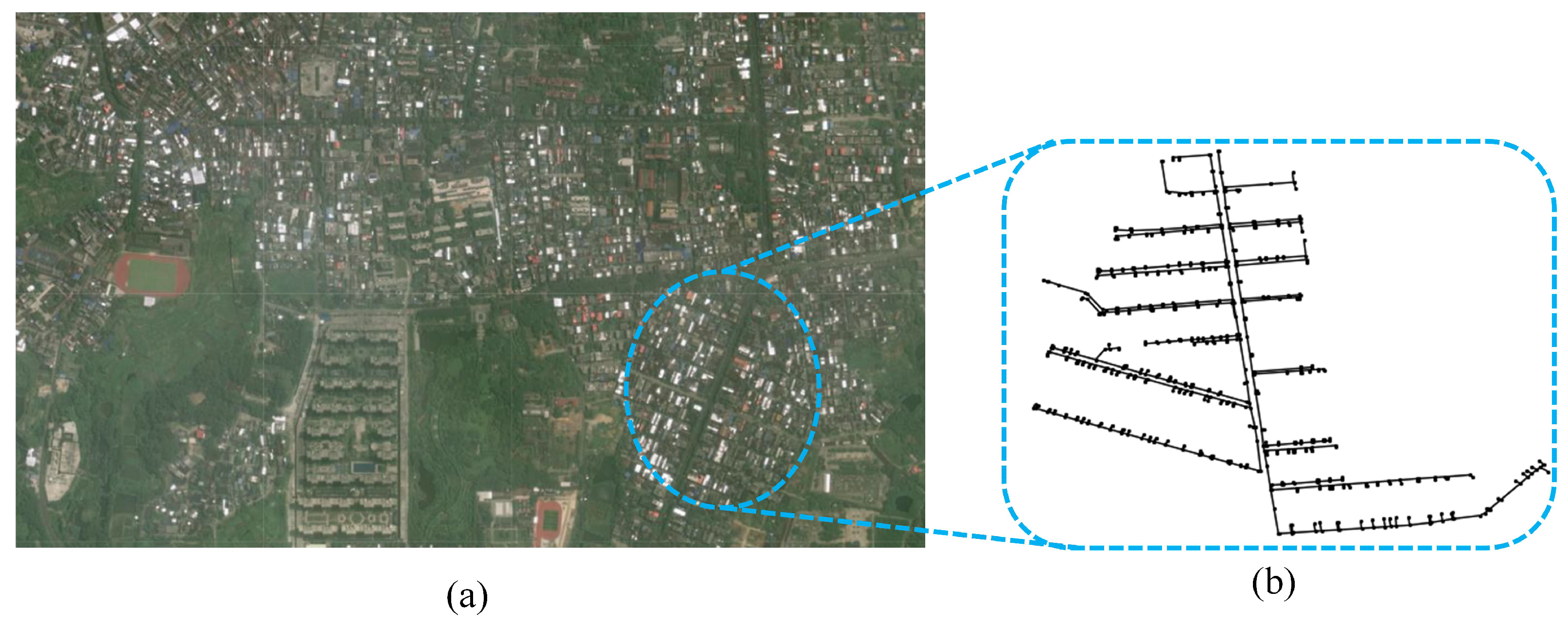
A real WDN was used to test the proposed method in real situations. The network is located in South China’s Hainan province. A DMA partition was selected for analysis. The longitude and latitude of the DMA are as follows: longitude—109.546409; latitude—19.514878. This DMA partition consists of 686 pipes and 688 nodes. The pipe length is 0.27–16.6 km, the pipe diameter is 32–100 mm, and the roughness coefficient is 140. The topology structure and location of the pipe network are shown in Figure 7.
The adjacency matrix A of the WDN was obtained according to the topology of the WDN, and the pressure sequence X of all nodes under normal operation was obtained using WNTR. The simulation time was set to 48 h, the sensor sampling interval was set to 15 min, and the size of the obtained feature matrix was 193 × 688. In the simulation, the total demand of each node is allocated to each node based on the historical water usage patterns from January 2024 to November 2024, forming the demand patterns of each node. Our demand scenario is based on the benchmark average daily demand. Although the data do not cover all seasons, the extreme months of summer and winter can well reflect its reliability. Then, the feature matrix was input into the auto-encoder for pre-training to obtain features.
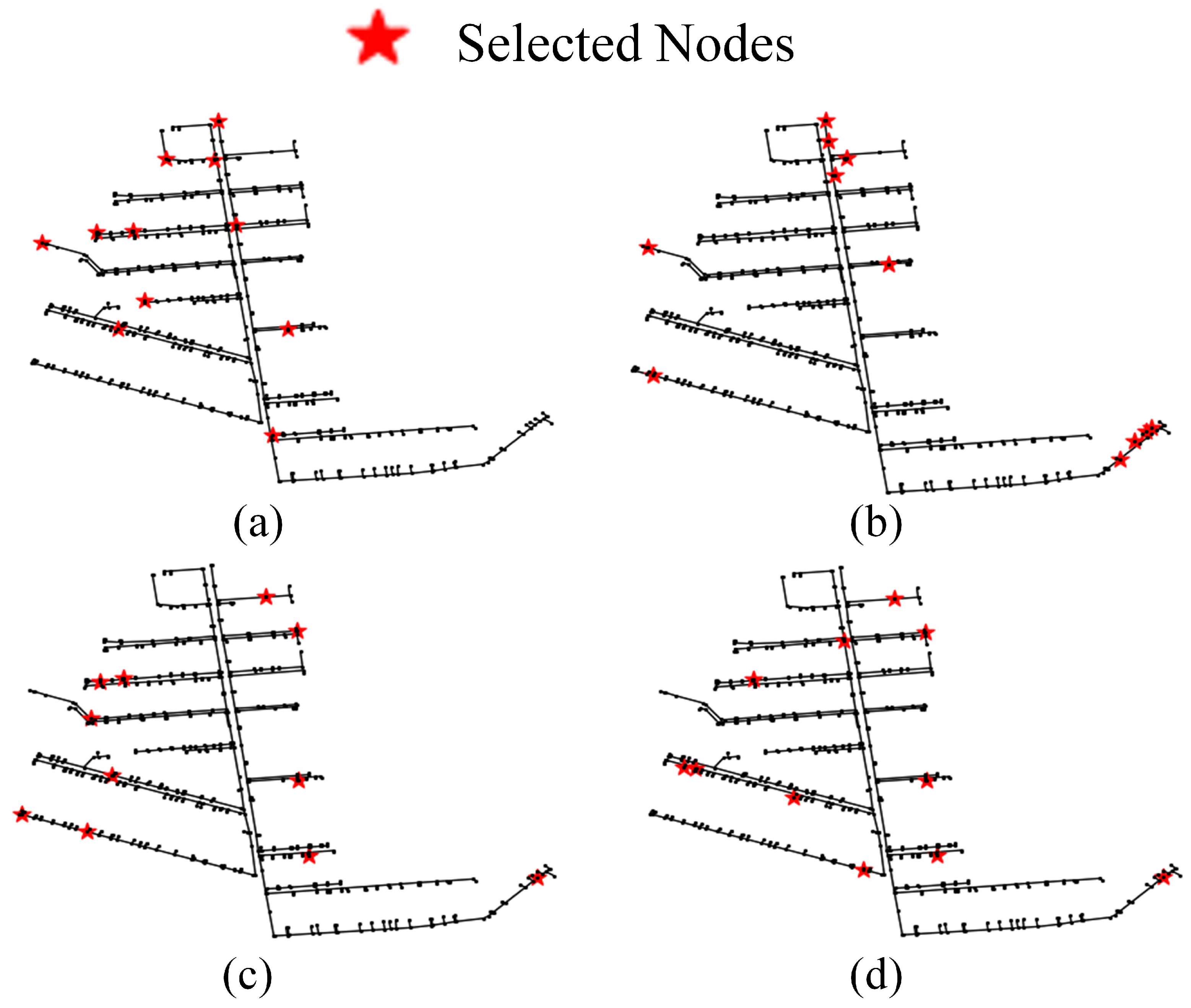
In order to prove the effectiveness of the proposed method, the most advanced SDCN algorithm, K-means algorithm, and the DBSCAN algorithm were selected for comparison. The K-means algorithm clustered the row vectors of the pressure leakage sensitive matrix, and selected the cluster center as the pressure monitoring point. The sensor layout results were shown in Figure 8a. The DBSCAN algorithm constructed a special node feature matrix for clustering, and selected the node with the greatest impact as the location of the monitoring point. The sensor layout results are shown in Figure 8b. The SDCN algorithm used the constructed graph neural network module and auto-encoder module to cluster nodes of the WDN. After the clustering was completed, the node with the highest perception rate of nodes in the region was selected as the pressure monitoring point, and the layout results were shown in Figure 8c. The layout results of our proposed method are shown in Figure 8d.
It can be clearly seen from Figure 8 that the pressure monitoring points arranged by our proposed method are more representative. The monitoring points arranged by the K-means algorithm are concentrated on the main road, which may affect the detection of end leakage. Part of the monitoring points arranged by the DBSCAN algorithm were distributed at the end of the pipeline, part were distributed on the main road, and part of the monitoring points were concentrated together, which will also affect the monitoring effect. This is because the DBSCAN algorithm is an algorithm based on density clustering. The nodes at the beginning and end of a pipeline usually have higher “uniqueness” or “irreplaceability” in terms of topology. This makes them more likely to become core points in density-based clustering. Compared with traditional methods, DBSCAN ensures the sufficiency and non-redundancy of sensors above the topological structure. There are six monitoring points arranged by the SDCN algorithm in the same position as the method proposed by us. But when SDCN arranged the left half of the pipe network, all the monitoring points were arranged at the end of the pipe network, and the monitoring points are evenly distributed in the main road and at the end of the pipe network in our method, which can achieve a more robust monitoring effect.
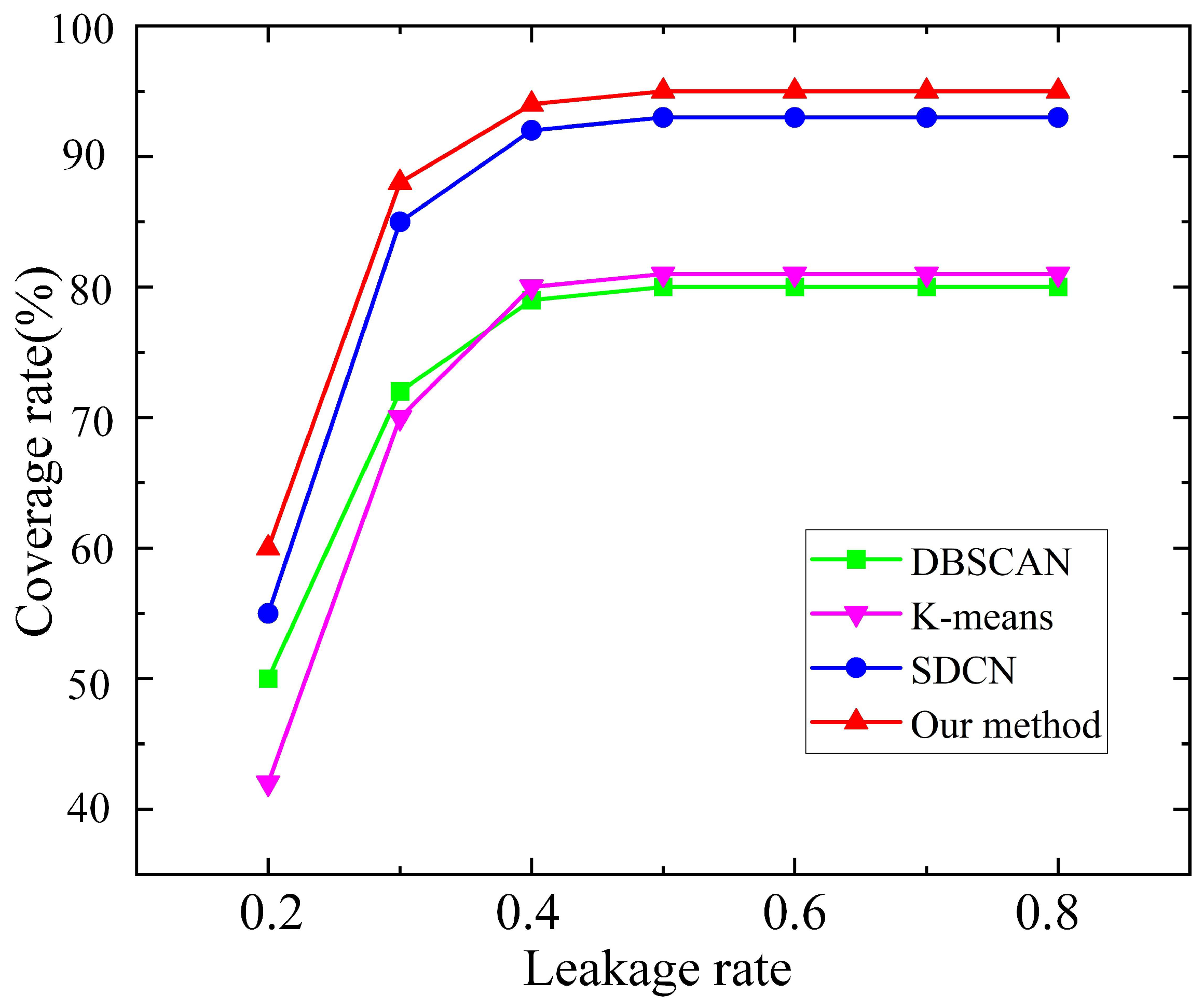
The two metrics in Section 3.1 were used to measure the usability and effectiveness of the proposed algorithm. We first create leakage rate = [0.2:0.8, 0.1] at different nodes of Wanfudong net and obtain time series data with a simulation time of 48 h and a sensor sampling interval of 15 min. The leakage rate has no unit. It is equal to the leakage diameter divided by the pipe diameter. A total of 688 × 7 sets of leakage data were simulated. These 4816 sets of data contain pressure values for all nodes. We calculate the coverage of the nodes of the pipeline network for different methods of arranging the pressure monitoring points with different leakage rates based on the locations of the pressure monitoring points. The coverage of the four methods under different leak sizes is shown in Figure 9.
As can be seen from Figure 9, our proposed method achieved the highest node coverage under all leakage sizes. The node coverage is 2% higher than the benchmark algorithm SDCN. This means that the proposed method in Wanfudong net can cover 14 more nodes than the SDCN algorithm, which can obtain a better monitoring effect. This is because the proposed method has arranged some sensors at the end of the pipeline to effectively monitor the hydraulic changes at the end of the pipeline. For leaks in the main pipeline, they can be sensed by the sensors arranged by conventional methods, but for leaks in certain end pipes with small diameters, it is difficult for the sensors arranged by conventional methods to detect them. This proves the superiority of our proposed method: not only is the monitoring of the main pipe considered, but also the monitoring of the end pipe. Redundant sensor arrangements are avoided.
The leak detection accuracy rate was tested to verify the effect of the pressure monitoring points arranged by the method in practical applications. We used the ResNet18 network as a classifier to test the leakage detection effect of pressure monitoring points arranged by four methods. In the test, we first used WNTR to simulate 1000 leaks of any size at any location as training data. For the simulation of these 1000 leaks, the leakage coefficient is configured to a range spanning from 0.2 to 0.8, where the leakage coefficient is equal to the leakage diameter divided by the pipe diameter, and we randomly select a number from this leakage range to conduct a leakage simulation for a random pipeline. Finally, 1000 sets of leaked pressure data were obtained. During training, we selected a batch size of 16 and obtained the training loss curve, as shown in Figure 10. After the training was completed, we simulated 1 leak per node as test data for a total of 688 leaks. The leak detection accuracy of each method is shown in Table 2.
It can be seen from the results in Figure 10 that the monitoring points arranged by the proposed method have better effects on leakage detection. The proposed method has already reached convergence at 170 training batches with a loss of 0.0024. The loss of the K-means method and the SDCN method fluctuated by 0.3 at batch 200, and it did not reach convergence. The DBSCAN method achieved convergence in batch 200. The data collected by the monitoring points arranged by these four methods on the training loss of ResNet18 can show the robustness of the data. A more reasonable location of the monitoring points can detect more leakage fluctuations and more obvious leakage features. Convergence can be reached faster when training the classifier. Therefore, more efficient data can train more accurate models, which can improve the accuracy of leak detection. This proves the better characterization of the data collected by the proposed method.
Table 2 shows that the leak detection accuracy of the proposed method is 9.77% higher than the K-means method and 6.77% higher than the DBSCAN method. It is 0.7% higher than the current most advanced SDCN algorithm. This performance benefits from two points: the excellent performance of the DBSCAN method demonstrates the importance of proper label initialization, and due to the introduction of the self-attention mechanism, the graph structure and node features of the pipe network obtain better weight distribution, improve the accuracy and rationality of clustering, and thus improve the accuracy of detection. In summary, compared with other schemes, the experimental results show that the proposed method has better performance both in terms of node coverage of the pipe network and leak detection accuracy. The proposed method can monitor pressure fluctuations at more nodes under different leak sizes, which is important for subsequent work on other pipe networks. In terms of leakage detection, the proposed method arranges pressure monitoring points with the highest leakage detection accuracy, which makes great progress in maintaining the stability of the water supply network and ensuring the residents’ water use.

4. Conclusions

In this paper, an intelligent algorithm for the optimal deployment of water network monitoring sensors based on automatic labelling and graph neural network (ALGN) was proposed. The issue of suboptimal clustering performance resulting from manual parameter configuration has been effectively addressed. It has been achieved that only by inputting the topological structure of the pipe network and the pressure information of nodes, the clustering results and the results of sensor layout can be obtained. Adaptivity is mainly reflected in two aspects: the dung beetle optimization algorithm (DBO) automatically determines the parameters of the density-based noise application spatial clustering (DBSCAN), and the attention mechanism adaptively allocates weights. We used the DBO algorithm to improve the DBSCAN method and obtain the initial labels and the optimal number of clusters for clustering, and the auto-encoder was used to obtain the higher-order feature representation of node hydraulic power. Then, the node hydraulic characteristics, network topology, and pre-trained high-order feature representation were input into the constructed network for training, and the loss function was constructed by a dual self-supervision mechanism to obtain clustering results. Finally, the cross-correlation distance was seen as the index, and the node with the smallest cross-correlation distance in the class was selected as the optimal pressure monitoring point. Two water distribution networks (WDNs) were selected for analysis to verify the effectiveness of the method. Case 1 proved that our proposed method considered both hydraulic characteristics and topology of WDN when clustering nodes. Case 2 analyzed a real WDN in southern China. Using node coverage and leak detection accuracy as indicators, the experimental results have shown that the proposed method is better than the most advanced methods in both node coverage and leak detection accuracy. The node coverage rate of this method has reached 93%, and the accuracy rate of leakage detection has reached 99.77%, both of which are better than K-means, DBSCAN, and SDCN. The method we proposed provided a feasible scheme for the layout of pressure sensors in WDN to guide engineering practice.
While the proposed method shows promising results, it has certain limitations. The algorithm’s performance relies on the quality and completeness of the hydraulic and topological input data. In addition, the current model may require substantial computational resources for very large-scale networks. And in actual situations, there exist real-world conditions such as hydraulic disturbances, reduced water demand, and rapid valve closure, which can affect the monitoring of leaks. Future research will focus on enhancing computational efficiency, integrating multi-objective optimization considering cost and reliability, and will focus on enhancing the robustness of the model in complex environments.

Author Contributions

Methodology, writing—original draft preparation, G.S.; supervision, X.W. and J.Z.; data curation, X.G. All authors have read and agreed to the published version of the manuscript.

Funding

This work was supported in part by Hainan Province Science and Technology Special Fund under Grant ZDYF2023GXJS159 and Grant ZDYF2023GXJS168.

Institutional Review Board Statement

Not applicable.

Informed Consent Statement

Not applicable.

Data Availability Statement

The dataset generated and analyzed during the current research period is divided into simulated data and real data. The hydraulic software analysis package that supports the generation of simulated data for this study is WNTR, which is a Python package compatible with EPANET designed to simulate and analyze the elasticity of water distribution networks. Can be in https://usepa.github.io/WNTR/index.html (accessed on 6 March 2025). Get it for free. Real data can be obtained from the corresponding author and licensed for free.

Conflicts of Interest

Author Xinlei Gao is employed by Guangdong Water Co., Ltd. The remaining authors declare that the research was conducted in the absence of any commercial or financial relationships that could be construed as a potential conflict of interest.

Abbreviations

The following abbreviations are used in this manuscript:
WDNsWater Distribution Networks
DBODung Beetle Optimization algorithm
DBSCANDensity-Based noise application Spatial Clustering
GCNGraph Convolutional Networks
SDCNStructural Deep Clustering Network
EGAEEmbedding Graph Auto-Encoder
EPANETEnvironmental Protection Agency Network Analysis Tool
MINPSTminimum number of points
EPSdomain radius of the sampling points
SAverage silhouette coefficient of the cluster
x i ( t ) The position of the i-th dung beetle at the t iteration
XThe current local optimal position
ZData representation of the hidden layer
HData representation of auto-encoders
YThe feature representation of the construction

References

  1. Chan, T.K.; Chin, C.S.; Zhong, X. Review of current technologies and proposed intelligent methodologies for water distributed network leakage detection. IEEE Access 2018, 6, 78846–78867. [Google Scholar] [CrossRef]
  2. Wang, T.; Liu, S.; Qian, X.; Shimizu, T.; Dente, S.M.; Hashimoto, S.; Nakajima, J. Assessment of the municipal water cycle in China. Sci. Total Environ. 2017, 607, 761–770. [Google Scholar] [CrossRef]
  3. Fontanazza, C.M.; Notaro, V.; Puleo, V.; Freni, G. Multivariate statistical analysis for water demand modeling. Procedia Eng. 2014, 89, 901–908. [Google Scholar] [CrossRef]
  4. Wu, Y.; Liu, S. A review of data-driven approaches for burst detection in water distribution systems. Urban Water J. 2017, 14, 972–983. [Google Scholar] [CrossRef]
  5. Li, R.; Huang, H.; Xin, K.; Tao, T. A review of methods for burst/leakage detection and location in water distribution systems. Water Sci. Technol. Water Supply 2015, 15, 429–441. [Google Scholar] [CrossRef]
  6. Ferreira, B.; Antunes, A.; Carriço, N. Multi-objective optimization of pressure sensor location for burst detection and network calibration. Comput. Chem. Eng. 2022, 162, 107826. [Google Scholar] [CrossRef]
  7. Di Nardo, A.; Di Natale, M.; Giudicianni, C.; Santonastaso, G.F.; Tzatchkov, V.G.; Alcocer-Yamanaka, V.H. Redundancy features of water distribution systems. Procedia Eng. 2017, 186, 412–419. [Google Scholar] [CrossRef]
  8. Wéber, R.; Hős, C. Efficient technique for pipe roughness calibration and sensor placement for water distribution systems. J. Water Resour. Plan. Manag. 2020, 146, 04019070. [Google Scholar] [CrossRef]
  9. Meier, R.W.; Barkdoll, B.D. Sampling design for network model calibration using genetic algorithms. J. Water Resour. Plan. Manag. 2000, 126, 245–250. [Google Scholar] [CrossRef]
  10. Zhou, X.; Tang, Z.; Xu, W.; Meng, F.; Chu, X.; Xin, K.; Fu, G. Deep learning identifies accurate burst locations in water distribution networks. Water Res. 2019, 166, 115058. [Google Scholar] [CrossRef]
  11. Wang, T.; Liu, Y. Optimization of pipe network pressure monitoring points based on hydraulic influence modification pressure monitoring point optimization. In Proceedings of the 2024 IEEE 6th International Conference on Power, Intelligent Computing and Systems (ICPICS), Shenyang, China, 19–21 July 2024; IEEE: Piscataway, NJ, USA, 2024; pp. 433–437. [Google Scholar]
  12. Cheng, W.; Chen, Y.; Xu, G. Optimizing sensor placement and quantity for pipe burst detection in a water distribution network. J. Water Resour. Plan. Manag. 2020, 146, 04020088. [Google Scholar] [CrossRef]
  13. Fei, J. Optimal arrangement of pressure monitoring points in water supply network based on intelligent optimization algorithm. In Hydraulic Structure and Hydrodynamics; Springer Nature: Singapore, 2024; pp. 451–461. [Google Scholar]
  14. Cheng, L.; Kun, D.; Tu, J.-P.; Dong, W.-X. Optimal placement of pressure sensors in water distribution system based on clustering analysis of pressure sensitive matrix. Procedia Eng. 2017, 186, 405–411. [Google Scholar] [CrossRef]
  15. Wang, F.; Bai, H.; Li, D.; Wang, J. Energy-Efficient Clustering Algorithm in Underwater Sensor Networks Based on Fuzzy C Means and Moth-Flame Optimization Method. IEEE Access 2020, 8, 97474–97484. [Google Scholar]
  16. Romero-Ben, L.; Cembrano, G.; Puig, V.; Blesa, J. Model-free sensor placement for water distribution networks using genetic algorithms and clustering. In Proceedings of the 10th IFAC Conference on Control Methodologies and Technology for Energy Efficiency (CMTEE), Toulouse, France, 11–13 November 2020; Volume 53, pp. 372–377. [Google Scholar]
  17. Wang, Y.; Tan, D.B.; Ye, S.; Hu, Z.K.; Yao, Z.L. Multi-criteria decision-making method for optimal sensor layout for leakage monitoring of water supply network. J. Changjiang River Sci. Res. Inst. 2024, 41, 178. [Google Scholar]
  18. Kipf, T.N.; Welling, M. Semi-supervised classification with graph convolutional networks. arXiv 2017, arXiv:1609.02907. [Google Scholar] [CrossRef]
  19. Peng, S.; Cheng, J.; Wu, X.; Fang, X.; Wu, Q. Pressure sensor placement in water supply network based on graph neural network clustering method. Water 2022, 14, 150. [Google Scholar] [CrossRef]
  20. Li, J.; Zheng, W.; Wang, C.; Cheng, M. Optimal sensor placement for leak location in water distribution networks based on EGAE clustering algorithm. J. Clean. Prod. 2023, 426, 139175. [Google Scholar] [CrossRef]
  21. Zhang, W.; Yang, X.; Li, J. Sensor placement for leak localization in water distribution networks based on graph convolutional network. IEEE Sens. J. 2022, 22, 21093–21100. [Google Scholar] [CrossRef]
  22. Zhou, X.; Wan, X.; Liu, S.; Su, K.; Wang, W.; Farmani, R. An all-purpose method for optimal pressure sensor placement in water distribution networks based on graph signal analysis. Water Res. 2024, 266, 122354. [Google Scholar] [CrossRef]
  23. Vittori, G.; Falkouskaya, Y.; Jimenez-Gutierrez, D.M.; Cattai, T.; Chatzigiannakis, I. Graph neural networks to model and optimize the operation of Water Distribution Networks: A review. J. Ind. Inf. Integr. 2025, 100880. [Google Scholar] [CrossRef]
  24. Bi, F.M.; Wang, W.K.; Chen, L. DBSCAN: Density-based spatial clustering of applications with noise. J. Nanjing Univ. 2012, 48, 491–498. [Google Scholar]
  25. Xue, J.; Shen, B. Dung beetle optimizer: A new meta-heuristic algorithm for global optimization. J. Supercomput. 2023, 79, 7305–7336. [Google Scholar] [CrossRef]
  26. Michelucci, U. An introduction to autoencoders. arXiv 2022, arXiv:2201.03898. [Google Scholar] [CrossRef]
  27. He, X.; Wang, B.; Hu, Y.; Gao, J.; Sun, Y.; Yin, B. Parallelly adaptive graph convolutional clustering model. IEEE Trans. Neural Netw. Learn. Syst. 2022, 35, 4451–4464. [Google Scholar] [CrossRef]
  28. Zhang, H.; Li, P.; Zhang, R.; Li, X. Embedding graph auto-encoder for graph clustering. IEEE Trans. Neural Netw. Learn. Syst. 2022, 34, 9352–9362. [Google Scholar] [CrossRef]
  29. Klise, K.A.; Hart, D.; Moriarty, D.M.; Bynum, M.L.; Murray, R.; Burkhardt, J.; Haxton, T. Water Network Tool for Resilience (WNTR) User Manual (No. SAND2017-8883R); Sandia National Laboratories: Albuquerque, NM, USA, 2017. [Google Scholar]
  30. Kingma, D.P.; Ba, J. Adam: A method for stochastic optimization. arXiv 2014, arXiv:1412.6980. [Google Scholar]
  31. Berardi, L.; Laucelli, D.B.; Ripani, S.; Piazza, S.; Freni, G. Using water loss performance indicators to support regulation and planning in real water distribution systems. Digit. Water 2025, 3, 1–20. [Google Scholar] [CrossRef]
  32. He, K.; Zhang, X.; Ren, S.; Sun, J. Deep residual learning for image recognition. In Proceedings of the 2016 IEEE Conference on Computer Vision and Pattern Recognition (CVPR), Las Vegas, NV, USA, 27–30 June 2016; pp. 770–778. [Google Scholar]
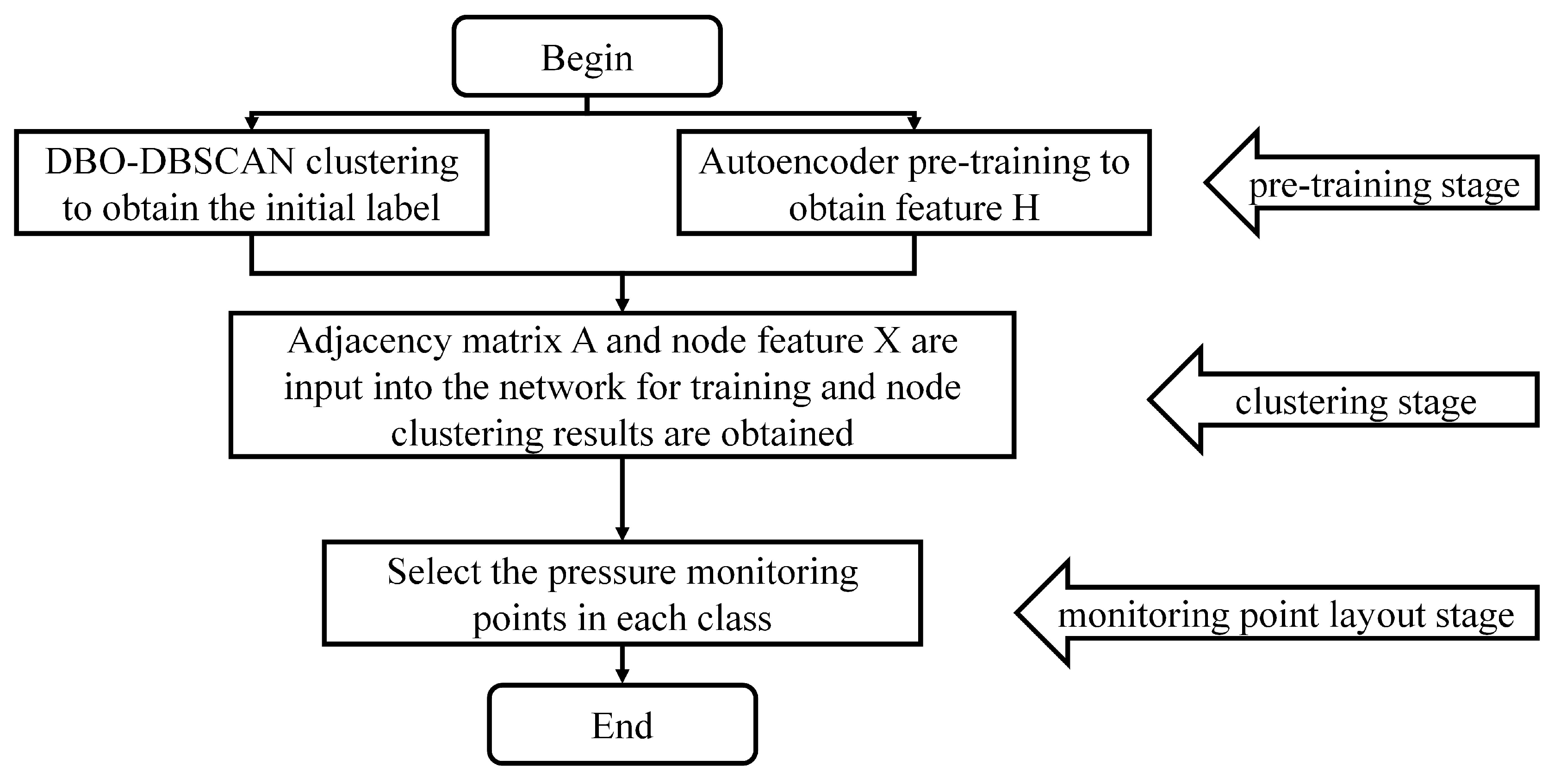
Figure 1. The flowchart of the ALGN.
Information 16 00837 g001
Figure 2. The flow block diagram of the DBO-DBSCAN algorithm.
Information 16 00837 g002
Figure 3. The framework of the ALGN.
Information 16 00837 g003
Figure 4. Self-attention module structure.
Information 16 00837 g004
Figure 5. (a) Topological structure; (b) reservoir demand pattern; (c) left demand pattern; (d) right demand pattern of the Simple net.
Information 16 00837 g005
Figure 6. Clustering results of the three methods: (a) our proposed method; (b) the DBSCAN method; (c) the K-means method.
Information 16 00837 g006
Figure 7. The location (a) and topology structure (b) of Wanfudong net.
Information 16 00837 g007
Figure 8. Pressure monitoring point layout results of Wanfudong net by four algorithms: (a) the K-means algorithm; (b) the DBSCAN algorithm; (c) the SDCN algorithm; (d) our proposed method.
Information 16 00837 g008
Figure 9. Coverage rate of the four methods (K-means, DBSCAN, SDCN, and the proposed method) under different leakage rate.
Information 16 00837 g009
Figure 10. Training loss curves of the four methods trained on ResNet18: (a) K-means; (b) DBSCAN; (c) SDCN; (d) our proposed method.
Information 16 00837 g010
Table 1. Node coverage rates of the four methods.
MethodNode Coverage Rates (%)
K-means83.3
DBSCAN87.8
SDCN94.4
The proposed method94.4
Table 2. Leakage detection accuracy of the four methods.
MethodAccuracy (%)
K-means90
DBSCAN93
SDCN99.07
The proposed method99.77
Disclaimer/Publisher’s Note: The statements, opinions and data contained in all publications are solely those of the individual author(s) and contributor(s) and not of MDPI and/or the editor(s). MDPI and/or the editor(s) disclaim responsibility for any injury to people or property resulting from any ideas, methods, instructions or products referred to in the content.