Article

Optimized Early Prediction of Business Processes with Hyperdimensional Computing

1
Computer Science and Engineering, University of California San Diego, La Jolla, CA 92093, USA
2
Electrical and Computer Engineering, San Diego State University, San Diego, CA 92182, USA
*
Authors to whom correspondence should be addressed.
Information 2024, 15(8), 490; https://doi.org/10.3390/info15080490
Submission received: 3 July 2024 / Revised: 10 August 2024 / Accepted: 12 August 2024 / Published: 16 August 2024
(This article belongs to the Special Issue Second Edition of Predictive Analytics and Data Science)

Abstract

:
There is a growing interest in the early prediction of outcomes in ongoing business processes. Predictive process monitoring distills knowledge from the sequence of event data generated and stored during the execution of processes and trains models on this knowledge to predict outcomes of ongoing processes. However, most state-of-the-art methods require the training of complex and inefficient machine learning models and hyper-parameter optimization as well as numerous input data to achieve high performance. In this paper, we present a novel approach based on Hyperdimensional Computing (HDC) for predicting the outcome of ongoing processes before their completion. We highlight its simplicity, efficiency, and high performance while utilizing only a subset of the input data, which helps in achieving a lower memory demand and faster and more effective corrective measures. We evaluate our proposed method on four publicly available datasets with a total of 12 binary prediction tasks. Our proposed method achieves an average 6% higher area under the ROC curve (AUC) and up to a 14% higher F1-score, while yielding a 20× earlier prediction than state-of-the-art conventional machine learning- and neural network-based models.

1. Introduction

A business process is a sequence of relevant events that involve a number of users and attributes that ultimately lead to a desirable outcome within a system [1]. Process mining is the field that aims to extract valuable insights about the behavior of processes by analyzing processes recorded in tabular data formats called event logs [1,2]. Process instances within an event log are also known as traces. Each trace comprises a non-empty sequence of chronological events (also known as control flow) and their corresponding attributes.
Recently, new techniques have been developed and used at run-time, i.e., during the execution of a process, for prediction and recommendation purposes before the process terminates [3]. Given an incomplete sequence of events, the desired prediction might include the probability of fulfilling a business constraint in terms of a logical rule within a time cycle [4], identifying the next event to be executed in the ongoing process [5], estimating the remaining time for process execution [6,7], or determining the event at which the process instance will terminate among the possible outcomes [8,9,10]. Predicting the outcome of incomplete traces is analogous to early sequence classification [11]. If an ongoing process is predicted to violate a predefined constraint or business rule, result in an undesirable outcome, or exceed the expected execution time, appropriate measures can be taken to mitigate adverse effects. For example, predicting the waiting time of a patient during the registration process can help in taking appropriate measures such as bypassing activities or allocating extra resources to expedite the registration process [12]. Another business example is the loan application process, wherein the process starts when an application is submitted and ultimately ends with a decision on whether the application is approved, rejected, or canceled. In this case the goal of the early prediction of the final decision is gaining optimized resource allocation and risk management in the early steps of the ongoing process. We are interested in early prediction, while actions can still be taken to prevent potential violations and correct the process’s direction at an early stage [13,14].
Many studies have sought to propose predictive process monitoring techniques for early prediction in incomplete process instances. Generally, a pair of “sequences of events in trace prefixes, events attributes” is taken as the input of a prediction model. These models are trained on feature vectors derived from historical traces and their associated labels and are used to predict the label of an ongoing trace from a predefined set of possible outcomes [1,15,16,17].
Amongst the most commonly used methods are gradient-boosted trees (XGBoost) [18,19], Random Forest (RF) [8], K-Nearest Neighbor (KNN) [9], Long Short-Term Memory (LSTM) [10,20,21], and att-Bi-LSTM [10]. Nevertheless, traditional machine learning methods do not consider the order of events in traces or store the patterns observed in sub-sequences of data. However, some methods, such as the index-based approaches in [22] or LSTM-based approaches [18] require the continuous updating of the feature vector length and reprocessing and training from scratch with the execution of every new event, making them computationally intensive. Neural network-based models require arduous hyper-parameter tuning, and a new model is needed when features are added or removed from the events, making them computationally inefficient. To increase the speed of training, data sampling methods have been proposed specially for large datasets [12]. But expensive and time-consuming calculations are required to choose the appropriate instances representing the whole dataset [21].
In this work, we focus on predicting the label of ongoing processes, which is referred to as outcome-oriented predictive process monitoring [1]. We introduce a novel approach based on Hyperdimensional Computing (HDC) [23] to the process mining community wherein, in addition to event attributes and control flow information, we incorporate patterns in sequences of events within traces. HDC encodes low-dimensional input data into high-dimensional representations called hypervectors [24]. The hypervectors preserve the distance of the original data in the high-dimensional space and enable learning tasks such as classification through simple operations. We use fixed-length feature vectors to store patterns and attribute information, supporting traces of arbitrary lengths. The encoding step is followed by training using element-wise operations on the hypervectors, where the hypervectors belonging to the same label (e.g., same outcome) are summed up (superimposed) together to generate their representative class hypervector. Inference involves encoding input data into a query hypervector and comparing it to a class of hypervectors using a similarity metric like the dot product or cosine distance. We train our proposed method with and without considering event attributes and show that our proposed methods outperform conventional ML-based and neural network-based methods including XGBoost [19] and LSTM [10,18] in terms of previous AUC values and F1-scores. Additionally, we illustrate that even using a random subset of the input data (without the need for compute-intensive data sampling in large datasets), our proposed method achieves a high performance. Our main contributions are as follows:
  • We propose a novel method for process outcome prediction based on Hyperdimensional Computing. Unlike conventional approaches, our method utilizes fixed-length vectors to maintain event patterns and attributes, effectively preserving memory. Also, unlike previous methods that require iterative encoding and training for prediction at different indices, in our proposed method, we adopt a novel approach wherein, for the observation of a new event or attribute, we add its corresponding hypervector to the previously constructed hypervector. This eliminates the need to encode and train an ongoing process from scratch.
  • Through eliminating traditional hyper-parameter tuning and incorporating a wise storage mechanism for subsets of trace prefixes, our proposed method enables the construction of a classifier on historical data using basic element-wise operations along vectors.
  • Choosing event attributes that determine the class of a process requires domain knowledge, but such information is lacking in many datasets. Therefore, we designed two algorithm versions: one, HDC-based, considers only patterns and event order within processes, and the other, attribute-based HDC (Att-HDC), considers patterns within sequence of events, event order, and event attributes.
  • The experimental results demonstrate the F1-score improving by up to 14% compared to the best baseline (XGBoost [19]) and AUC scores improving by an average of 6% in the key early process stages. This highlights the algorithm’s ability to provide more accurate predictions early on, without sacrificing runtime efficiency. Furthermore, we showcase our proposed method’s high performance when training on a randomly chosen subset of the input data, eliminating the need for compute-intensive sampling methods. Our proposed method yields a similar F1-score and AUC score with only a sampling ratio of 0.5 of the training data. Thus, we propose more accurate early prediction, eliminating the need for passing over the whole training data.
The rest of this paper is organized as follows: Section 2 presents the outcome-oriented predictive process monitoring and an overview of Hyperdimensional Computing. Related works are discussed in Section 3. Section 4 presents our HDC-based approach that integrates additional event pattern information for predicting the outcome of an ongoing business process. Section 5 evaluates the advantages of our proposed approach through experimental studies. Finally, Section 7 draws the conclusion and outlines future work.

2. Background

In this section, we first explore the key concepts and terminologies related to early outcome prediction in processes. Then, we introduce Hyperdimensional Computing.

2.1. Outcome-Oriented Predictive Process Monitoring

Definition: The goal of outcome-oriented predictive process monitoring is predicting, as early as possible, how an ongoing process instance will terminate based on the execution records of processes stored in event logs [1]. This information helps businesses in different areas such as risk mitigation and increasing performance in processes [3]. A trace in an event log is a sequence of chronological events. Each event has a unique identifier in a given event log and is associated with a timestamp that is later used to determine the order of events. An event’s features, also called event attributes, may include categorical and numerical data such as the associated resource, device, person, or the cost of the activity [25]. Each trace in an event log also has a unique trace identifier. Additionally, a trace can carry attributes related to the entire process instance.
Predictive Process Monitoring Framework: Within a trace, the sequence of events and their associated attributes are analogous to independent attributes in machine learning algorithms. The corresponding variable label (classes) can be any label from the set of possible outcomes. Trace labels are often determined based on their terminating events. A label can also be determined using a labeling function based on a set of logical rules. The rules can include analyzing the presence of a combination of events within a process that lead to the desired label or specific order of particular events. First, control flow information and event attributes in traces are mapped to feature vectors [19]. Control flow refers to the sequence and order of events. The event attributes include characteristics of each event, e.g., the agent in charge, resource, and cost. Later, these feature vectors are used as inputs for the classification models. Generating classification models is often referred to as offline step. During the execution of an ongoing process, often referred to as online step [19], the ongoing process is mapped to a feature vector similar to the training data, then the classification models trained in the offline mode are used for classifying it. In our proposed method, we first encode an ongoing query trace to a high-dimensional vector, using the same method applied to the training data. Then, the query vector’s label can be predicted as either of the possible outcomes using the trained classifier model.
Example: Table 1 depicts three randomly selected traces in a real event log that is commonly used in the literature, BPIC 2019  [26]. This dataset includes the history of purchase processes, and the early prediction is concerned with whether the application terminates as approved, rejected, or canceled. Events in this event log are associated with the Event Name, Timestamp, Resource and User, and Cumulative Net Worth (EUR) attributes.
In Table 1, trace 338, with five events, can be represented as [ e 338 , 1 , e 338 , 2 , e 338 , 3 , e 338 , 4 , e 338 , 5 ] . Since we aim at predicting the outcome of incomplete traces, we use the prefixes of the ongoing traces instead of the completed ones. A prefix of this trace is a sequence of events with an arbitrary length. For example, [ e 338 , 1 , e 338 , 4 ] , corresponding to [Create Purchase Order Item, Record Invoice Receipt], is a prefix with length 2 in trace t r a c e 338 . In event log BPIC 2019 , following common practice in the field, we define the trace labels based on whether the trace terminates with the event Clear Invoice (positive) or not (negative), resulting in a binary classification. As a result, both t r a c e 338 and t r a c e 198181 are labeled as positive as they terminate with Clear Invoice event, whereas t r a c e 529 is labeled as negative.

2.2. Hyperdimensional Computing

Hyperdimensional Computing (HDC) is a novel computational approach that encodes a d-dimensional input data point x R d into a high-dimensional vector, denoted by H . Hypervectors are the basis of HDC, and their dimension is denoted by D , where d D , and is often set to be 2000–10,000 [23,24]. These encoded hypervectors are composed of independent and identically distributed ( i . i . d . ) elements [23]. A useful mathematical property in the high-dimensional space (also known as hyperspace) that HDC benefits from [23] is that when given a set of i.i.d. hypervectors H α , H β , and H γ , their summation H Σ = H α + H β + H γ is closer to H α , H β , and H γ than any other randomly selected vector in the hyperspace. This property can be used to represent classes (sets of elements with the same label) by bundling encoded data points of a particular class through simple summation. The resultant class hypervector is, in expectation, similar to the associated data points. Also, in hyperspace with a large enough dimension, any two randomly chosen hypervectors are nearly orthogonal to each other [23].
The HDC learning framework comprises three steps, as depicted in Figure 1. First, each sample of a given input dataset, i.e., a trace with a set of events and corresponding event attributes is encoded into a D -dimensional hypervector. Determining an appropriate encoding algorithm is critical for this step. Based on the literature, n-gram encoding is often used in sequential data such as language [27] and DNA sequencing [28] where there is a spatiotemporal relationship between features [29]. Hence, in these sequential data types, n-gram encoding often yields higher performance compared to other encoding methods [27,29], so we use n-gram encoding as our encoding method.
A class of data representing a specific category of information (e.g., all business traces with the same label) is labeled using a class label, e.g., label positive or negative (e.g., terminating in a particular event or not). A single hypervector represents a class. To create the class vector, encoded hypervectors belonging to that label are superimposed (bundled) simply through dimension-wise addition to form class hypervectors.
A class of data representing a specific category of information (e.g., all business traces with the same label) is labeled using a class label, e.g., label positive or negative (e.g., terminating in a particular event or not). A single hypervector represents a class.
Third, with a set of n class hypervectors C 1 , C 2 , , C k , the HDC approach classifies a query process x q first by mapping it into a hyperdimensional representation and then finds out how similar the given query vector is to any of the k classes using a similarity metric δ such as the cosine distance or dot product [24].
The operations in the HDC steps are simple (mostly binary or integer addition or multiplication) and highly parallelizable, as operations on hypervector dimensions are independent, e.g., the addition of two hypervectors can be run in parallel over all of the D dimensions. Hence, in many applications, it can achieve several orders of magnitude speed-up compared to classic machine learning techniques [30]. In some cases, HDC has been empirically shown to require less labeled training data than other machine learning techniques [31,32]. The latter feature enables implementing HDC in problems with insufficient data for other algorithms. We also need to remark that HDC does not need the costly hyper-parameter tuning required in neural networks [33].
Hyperdimensional computing has been successfully applied to a wide range of data types including sequential data such as DNA sequencing [28] and text [27], image datasets [34], time-series datasets such as seizure detection [35], and for different tasks such as classification, clustering, and regression. Table 2 provides a summary of some of HDC’s applications in different domains. To the best of our knowledge, this is the first study that deploys a Hyperdimensional Computing-based method in the Predictive Process Mining Field. To perform a thorough analysis, we experimented on four benchmarks conventionally used in the literature within this domain, which we discuss further in Section 5.

3. Related Work

Traditional machine learning models that are widely used in predictive process mining adopt different procedures in the choice of the input data in the mapping control feature encoding phase. Ref. [22] selects all events up to the prediction state and, using the occurrence count of an event observed in a sequence, creates frequency-based vectors, ignoring the order of events and their attributes. In other studies such as [4], only the event attributes of the event at which the prediction is made are used as input data. Considering merely trace attributes instead of event attributes or the attributes of the last k events is the other approach discussed in [1]. On the other hand, Ref. [15] uses a combination of the order of events and attributes, which takes care of both the control flow and events features. However, the feature vector length is continuously updated as new executed events are being added to the prefix, impeding the use of a fixed-length feature vector. Once traces of events are represented as feature vectors, a classifier is trained on the feature vectors [8]. Among the most conventional machine learning-based techniques used are Random Forest (RF) [8], Gradient-Boosted Trees (XGBoost) [19], Support Vector Machines (SVM) [39], and Logistic Regression (LR) [19]. In the aforementioned methods, for prediction in different prefixes, a new model is needed to be trained.
More recently, NN-based methods including [10,19] use neural network-based techniques for outcome prediction, which consider the sequence of events as well as event attributes. The authors of [10] use Attention-based Bidirectional LSTM (Att-Bi-LSTM), which is a combination of a bidirectional long short-term memory neural network and an attention layer mechanism. However, similar to the other neural network-based algorithms, the proposed LSTM-based method in [10] requires hyper-parameter tuning in model creation, which can be complex and time consuming. Moreover, different datasets might need customized models, making the prediction even more challenging [40]. Also, it requires constant training in a trace for continuous predictions in different states of the given trace.
We present a novel approach for outcome prediction in ongoing traces based on Hyperdimensional Computing that will be further discussed in the following sections. Our method eliminates the need for encoding and training an ongoing process from scratch using single-pass inference. Also, our proposed method inherently eliminates the need for time and compute-intensive hyper-parameter tuning and is capable of yielding high performance, while in the initial steps of a process. We conducted a series of experiments to compare the efficiency and performance of our proposed method with the best state-of-the-art methods, namely, RF [8], XGBoost [19], SVM [39], and LR [19]. We also used a variation of LSTM, i.e., Att-bi-LSTM [10], which yields better performance than the conventional LSTM studied in [21].

4. HDC-Based Framework for Predicting Process Outcomes

In the following, we elaborate on the three main steps of Hyperdimensional Computing in the context of predicting the process outcome, namely encoding, training, and inference (prediction). We first introduce our proposed HDC algorithm which merely considers the patterns in sequences of events, and later, we introduce attribute-based HDC (Att-HDC), which, in addition to patterns in sequences of events, considers event attributes and has an additional step in the encoding compared to the HDC-based method. This section finally ends with the framework for the proposed Att-HDC algorithm. Table 3 summarizes the notations used throughout this paper.

4.1. Encoding

The first phase in the HDC framework is mapping input data into a hypervector. As mentioned earlier, we use patterns in sequences of events and event attributes to create feature vectors. We extract the unique IDs of events across the entire event log. Similarly, we store the unique attribute values of each event from all traces within the event log.
We map each unique event e i to a random D -dimensional binary hypervector in the hyperspace, dubbed an ID hypervector, denoted by H e i = { ± 1 } D . ID hypervectors are alternatives of scalar values in the hyperspace. Note that events are qualitative, i.e., the comparison of events is meaningless without any domain knowledge. For instance, two particular actions (events) of “Record Invoice Receipt” and “Record Goods Receipt” might be used interchangeably in a dataset or might have close meaning, so if the domain knowledge implies this, we expect that their mapping hypervectors should also preserve this proximity, i.e., H e i · H e j > 0 . However, due to the lack of such domain knowledge, we assume that no similarity is considered between any two H e i and H e j in the high-dimensional space; hence, H e i · H e j = 0 . Thereby, we do not need to store the proximity of events.
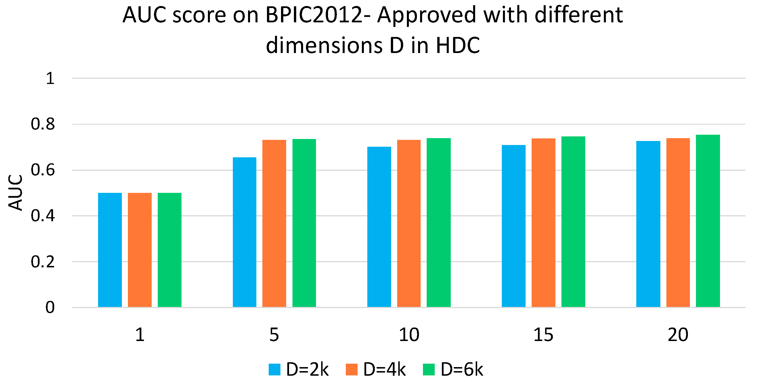
We illustrate our procedure on a real-life example by running it in our framework. We consider trace t 198181 in Table 1 as our ongoing example. This trace consists of four events and terminates in the ‘Clear Invoice’ event. It can be represented as [‘Create Purchase Order Item’, ‘Record Goods Receipt’, ‘Create Purchase Order Item’, ‘Clear Invoice’]. Based on Table 1, each of the events in this dataset has four attributes, namely ‘Event Name’, ‘Timestamp’, ‘Resource and User’, and ‘Cumulative Net Worth’. We first map each of the event names into the hyperspace. This step is performed by randomly mapping each unique event name into a D (here, 4000)-dimensional hyperspace. We experimented with different values of D and did not observe significant difference in the prediction results. Figure 2 in Section 5 illustrates results of deploying the method using different dimensions. We later show in the attribute-binding Section 5 thew difference of taking a similar measure for the ‘Resource and User’ categorical attribute. The encoded event would be H ( e i ) = { 0 , 1 } D wherein D stands for the dimension of the hyperspace. Each of the coordinates of the hypervector is equally likely to be 0 or 1. This randomness ensures that the dissimilarity of different event names is preserved and variant events are mapped into distinguishable representations, as each pair of randomly generated vectors is orthogonal.
Although we might have complete sequences during the training, predictions are aimed to be performed at event k of the query trace x q , i.e., before its termination. Thus, during encoding, prefixes of length k are extracted from historical traces as well. Therefore, for a historical trace t i , the prefix λ i of length k that starts from the first event in the trace is λ i = [ e i , 1 , , e i , k 1 , e i , k ] . Traces within the training and test data can be of any arbitrary and dissimilar lengths to each other. If k is equal to or more than the length of a trace t i of length m, the last m 1 events of the trace are considered the prefix. The reason for choosing m 1 events in such traces is that we want to make sure to perform the prediction before the end of a trace rather than on or after its termination. Similarly, for encoding historical traces, we disregard their last event (process outcome).
As explained in Section 2, HDC can represent a set by simply adding up the hypervectors of the comprising elements of that set. Thus, we can represent event prefix λ i by Equation (1). Such encoding, however, is not able to retain the temporal information of the sequences (order/pattern of events), i.e., H ( [ e A , e B , e C ] ) = H ( [ e C , e A , e B ] ) .
H ( λ i ) = j = 1 k L e i , j
To preserve the patterns of events in a prefix λ i , we split the prefix to sub-sequences of length n, called n-grams. The selection of n is tentative, but for the majority of applications, n { 3 , 4 } yields good accuracy. However, we experimented with different values of n for n-grams, and no significant difference was observed. In Section 5 we show the impact of several values of n on the performance of our proposed HDC method. We set the step of the n-gram encoding to be 1 to preserve all possible patterns of length 3. To encode a tri-gram ω j = [ e j , e j + 1 , e j + 2 ] , we applied a permutation-based (circular shift) encoding on its events. The permutation operation, by rotating the hypervector coordinates and generating dissimilar vectors to the origin by scrambling the original vector, is used for storing a sequence of hypervectors [41]. We denote the left permutation of elements of a sequence S = ( s 1 , , s m ) by P l ( S ) , wherein l means permutation by l indices, i.e., P ( 2 ) ( s ) = ( s 3 , , s n , s 1 , s 2 ) . Accordingly, the encoding of each tri-gram of events is calculated as
H ( ω j ) = l = 0 2 P l H ( e j + l )
That is, the ID hypervector of all three events in the tri-gram is selected and is permuted by 0, 1, and 2 for the first, second, and third event, and added up to form H ( ω j ) . To preserve the sequence of events, we need to perform a left rotation on different indices. Starting from the first event of a prefix, the tri-grams are encoded. Each of the events in a prefix is the starting event of a tri-gram.
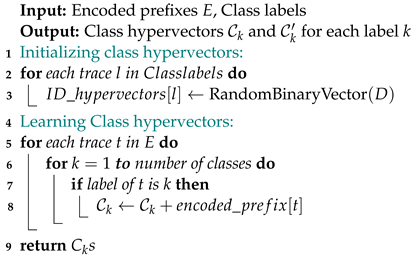
The encoding hypervector of the whole prefix with k events, H ( λ i ) , is produced by adding up all the k 2 encoded tri-grams (e.g., in a trace of length k = 3 , there is only one tri-gram). Algorithm 1 illustrates the pseudo-code for the encoding process.
H ( λ i ) = j = 1 k 2 H ( ω j )
Algorithm 1: HDC Encoding Algorithm
Information 15 00490 i001
Algorithm 2: Function: LeftRotate
   Input: Vector v e c t o r , Number of positions p o s i t i o n s
   Output: Vector rotated left by p o s i t i o n s indices
1  return  v e c t o r  rotated left by p o s i t i o n s indices
Algorithm 3: Function: RandomBinaryVector
   Input: Dimension D
   Output: A D-dimensional vector with random binary (0 or 1) elements
1  return A D-dimensional vector with random binary elements

4.2. Single-Pass Encoding and Inference

The encoding technique outlined above only visits each prediction index (input sample) once for different prefixes. In case a new event k + 1 is added to the prefix, as encoding is all about bundling the tri-grams, we only need to encode the tri-gram of ω k 1 = [ e k 1 , e k , e k + 1 ] and add the result to the existing encoding hypervector.
H ( λ i , k + 1 ) = j = 1 k 1 H ( ω j ) = j = 1 k 2 H ( ω j ) + H ( ω k 1 ) = H ( λ i , k ) + H ( ω k 1 )
Therefore, HDC only needs to store the last two observations along with the encoded hypervector. This impedes encoding and training from scratch for each inference, as opposed to conventional methods where the feature vector and learned model must adjust with each new event and attribute. Therefore, our proposed HDC-based methods result in lower computation and time consumption in continuous prediction across various prefix lengths.

4.3. Training

We built a classifier by running a binary classification algorithm for each label. To this end, we first encoded each and every input sample (prefix) using Equation (3). Then, we added all encoded hypervectors with the same label, e.g., in the BPIC 2019 dataset, the class hypervector of ‘Clear Invoice’ traces is the aggregation of hypervectors of all prefixes terminating in ‘Clear Invoice’ event. The class hypervector is a single hypervector that represents all prefixes with the same label.
C k = i s . t . y i = k H ( λ i ) C k = i s . t . y i k H ( λ i )
Since we formed it as a binary classification task (to concur with the literature), the complement class hypervector C was the aggregation of traces not terminating in the ‘Clear Invoice’ event. Algorithm 4 illustrates the pseudo-code for the the training phase.
Algorithm 4: HDC Training
Information 15 00490 i002

4.4. Inference (Prediction)

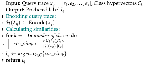
The ultimate goal is to predict the label of an incomplete trace. Assume that the last observed event in an ongoing trace x q is e k . To begin, we need to encode the x q = [ e 1 , e 2 , , e k ] query trace with the same procedure used for encoding the training traces. Then, we compare the resulting hypervector H ( λ q ) to all of the k class hypervectors. For measuring similarity, we use the cosine similarity (normalized dot product) metric, which is commonly used in the HDC field [42]. The cosine of the angle θ between vectors e n c ( x q ) and class C k is defined as follows:
c o s ( H ( λ q ) , C k ) = < H ( λ q ) , C k > | H ( λ q ) | | C k |
The label of the query is determined by the class with the highest similarity to the encoded query hypervector.
l q = a r g m a x k C δ ( H ( λ q ) , C k )
The above equation simply returns the predicted label l q for query trace x q . Here, δ is the cosine distance. The pseudo-code for the inference phase is shown in Algorithm 5.
Algorithm 5: HDC Inference
Information 15 00490 i003

4.5. Retraining

In contrast to deep neural networks that need tens of iterations (epochs) over the train data, the HDC algorithm achieves reasonable accuracy by visiting each input data point only once. However, the HDC accuracy can also be improved using a few retraining epochs at run-time. During the retraining, an inference is conducted between the training data and already-created class hypervectors. In case the class of a training query trace is predicted incorrectly, we add the encoded query process H ( λ q ) to the true class hypervector and subtract it from the incorrectly predicted class. If we denote the true class as C t and the falsely predicted one (complement of C t in binary classification) as C f , the retraining entails that
C t = C t + H ( λ q ) C f = C f H ( λ q )
Intuitively, this equation makes the incorrectly classified trace closer to the correct class and simultaneously increases the dissimilarity between the incorrect class and the query trace based on the set property of hyperspaces discussed earlier.

4.6. Attribute Binding in Att-HD

In an event log, each event contains attributes. These attributes might be categorical or numerical, and the values associated with event attributes in a given trace might affect determining its outcome. Hence, besides the HDC algorithm, we propose Att-HDC, which, in addition to a sequence of events in traces, takes the attributes of the events into account for creating feature vectors. Att-HDC is similar to HDC and only has an additional step compared to the HDC’s encoding phase. Hence, encoded feature vectors in the HDC algorithm can be easily converted to Att-HD. We treat the encoding of categorical attributes like unique event encoding. Let { a t t r 0 , a t t r 1 , , a t t r k } be the set of unique event attributes across all traces in an event log. We assign each unique attribute a random D -dimensional hypervector in the hyperspace. If the attribute is in a given range of numerical values ( v m i n , v m a x ) , we cannot consider i . i . d vectors for each of the given values as we need to preserve the proximity of similar values in the hyperspace. In order to impede creating various vectors for unique values, we need to quantize the attribute value range into Q = 100 bins and create “level hypervectors” for each of these quantized bins and preserve the proximity of close values. We set Q = 100 as our data range was large and our proposed method yields a slightly better AUC and F1-score with Q = 100 . The first quantizer receives L 0 = { ± 1 } D . The second quantizer L 1 is generated by flipping D 2 Q randomly chosen coordinates of L 0 . For example, if D = 10 , 000 and Q = 100 , then L 0 and L 1 will differ in 100 coordinates. Similarly L 2 is generated by randomly flipping D 2 Q coordinates of L 1 . Hence, the expected similarity (dot product) between L 0 and L j decays to zero. This insures that two similar values are mapped to similar hypervectors. These encoded attributes are later bound with the hypervector of the event that contains them. Thereby, if we consider H e i , j as the hypervector associated with event j in trace i, the t hypervectors associated with its attributes are summed up and added to its hypervector as follows:
H e i , j : = H e i , j + s = 1 t L i , j , s
For example, in Table 1, for ‘Cumulative Net Worth’, which contains numerical attributes, L 0 and L Q 1 are hypervectors associated with the values 0 and 1833, respectively, and are orthogonal to each other. After mapping the attributes, we need to bind each event attributes to itself. Then, for the first event in this dataset, we sum the hypervectors corresponding to ‘Create Purchase Order Item’, ‘user-119’, and ‘15.0’ together. We perform the same thing for the subsequent events and finally, by shifting the hypervectors of the events in the sequence, create the hypervector associated with the given trace.
We use timestamp information to maintain the chronological order of events in processes. Moreover, we exclude attributes that are significantly different across different events within processes as they do not help in identifying similar processes, i.e., processes with the same label. In Algorithm 6, we show how events are encoded when attributes are considered in the Att-HDC algorithm. Algorithm 6 uses Algorithms 2 and 3 respectively for generating random binary vectors and left rotation.
Algorithm 6: Att-HDC attribute binding
Information 15 00490 i004

4.7. Proposed HDC-Based Framework

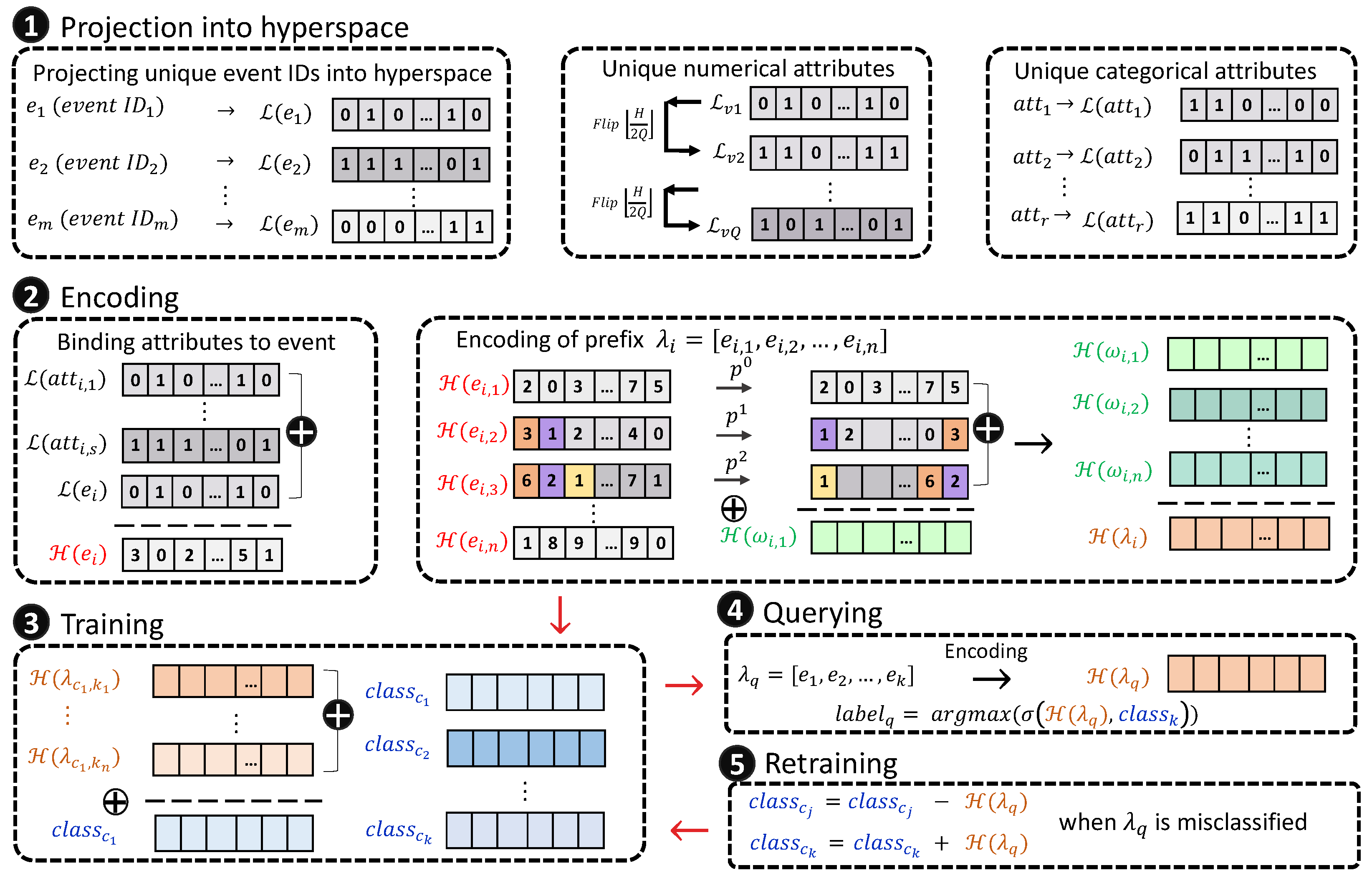
Figure 3 illustrates an overview of the proposed Att-HDC classification method. The first step is encoding, where unique events are mapped into the hyperspace of size D. Categorical event attributes are mapped to the hyperspace in a similar manner. For numerical values, quantization is conducted as discussed in Section 4.6. Then, after binding attributes vectors with event vectors for a given trace t i , sequences of length 3 (tri-grams) are chosen. After applying permutation on the elements of each tri-gram, they are summed up. The last phase in encoding is summing all such tri-grams to represent the trace i in the hyperspace. HDC differs only in that it does not bind attributes hypervectors to the event hypervectors.
In the second phase (training), traces of the same label are aggregated using a simple element-wise summation to create class hypervectors. Eventually, in the query phase for classifying an prefix λ q in an ongoing trace x q , after encoding it to H ( l a m b d a q ) , a similarity metric is calculated between the encoded prefix and the class hypervectors. In the retraining phase, the hypervector of a wrongly classified trace is added to the class hypervector it belongs to and is subtracted from the class hypervector it is mistakenly labeled as, to increase the prediction accuracy in further predictions. The proposed framework is independent of the event logs, meaning that we can implement a similar framework for any other event log with any number of unique events, traces, or classes and attributes upon obtaining the chronological event i d s of its traces. We present the pseudo-code for the proposed HDC and Att-HDC methods in Algorithm 1.

5. Experimental Evaluations

In this section, we discuss the datasets we used and the comprehensive series of tests we devised to evaluate our proposed method’s effectiveness as an accurate yet efficient means for predicting the label of an ongoing process instance using historical data. Our goal was to demonstrate that HDC attains superior performance than other techniques previously proposed in the literature. We measured our proposed method’s performance based on the F1-score, AUC score, and earliness and compare our proposed methods with XGBoost [19], RF [8], SVM [39], LR [19], and Att-bi-LSTM [10].

5.1. Datasets and Labeling Functions

We used four publicly available real-life process datasets from the Business Process Intelligence Challenge (BPIC), widely used in the literature, (1) BPIC 2012 , (2) BPIC 2015 , (3) BPIC 2017 , and (4) BPIC 2019 , to evaluate the performance of our method. For classification purposes, we followed the same procedure taken in previous studies for labeling traces [8,21]. Previous studies treat the outcome classification as a set of separate binary classifications instead of multi-label classification. In these datasets, several labeling functions are required for determining classes of traces. For instance, in BPIC 2012 Approved , the binary classifier determines whether each ongoing trace terminates as Approved or not terminating in any of the other possible outcomes. We defined a total of 12 binary classifications across all of the datasets:
(1)
The BPIC 2012 event log represents the history of loan application processes in a Dutch financial institute. Based on the literature, we define three labels for this dataset: BPIC 2012 Approved , BPIC 2012 Cancelled , and BPIC 2012 Declined , corresponding to cases terminated as approved, cancelled, or declined.
(2)
BPIC 2015 consists of five datasets provided by Dutch municipalities, containing event logs of building permit application processes. For labeling processes, the following Linear-time Temporal Logic (LTL) rule based on the literature is applied in each dataset i, where i { 1 , 2 , , 5 } denotes the number of the municipality: “ BPIC 2015 i :   φ = G (send confirmation receipt) → F(retrieve missing data)”, where φ is the LTL rule, and the label is 0 if φ is violated in the trace, and 1 otherwise. Operator G means that the activity should always hold in the subsequent positions of a path, and F means it should finally hold somewhere in the subsequent positions of a path. GF is the conditional propositions ( p q ). It expresses that if the confirmation receipt is always being sent, the missing data should be eventually retrieved.
(3)
The BPIC 2017 event log is an extended version of BPIC 2012 with richer and cleaner data. Similar to BPIC 2012 , we define three labels referred to as BPIC 2017 Approved , BPIC 2017 Cancelled , and BPIC 2017 Declined for processes terminating in approved, canceled, and declined events, respectively.
(4)
BPIC 2019 is collected from a large multinational company in the Netherlands and contains the handling of a purchase order. We label traces in this event log based on whether they terminate in the “Clear Invoice” event or not.
Table 4 presents the event log statistics such as the frequency of labels (classes), information regarding the length of traces, and the number of unique events and their unique attributes used across each event log. We consider patterns in the sequence of events (the control flow) and event attributes as input data. We discard the attributes that have the same value in all the traces as they do not contribute to better classification. Also, attributes with different values in all or most of the traces are discarded as uninformative.

5.2. Evaluation Metrics

We mainly use the F1-score, AUC (area under the ROC curve), time consumption, and earliness, which are the common metrics used to evaluate the performance of a classifier in predictive process monitoring [1] to evaluate the effectiveness of our classifier. We also report the execution time analysis during the ongoing prediction (aka online phase). We consistently use hypervector lengths of D = 4 k through the experiments as we observed it saturates the accuracy.
F1-score is referred to as the golden standard in the literature, represents the correct labeling of a trace [16]. The prediction outcome for an ongoing trace can be TP (true positive; correctly predicted as positive), TN (true negative; correctly predicted as negative), FN (false negative; falsely predicted as negative), or FP (false positive; falsely predicted as positive). The F1-score is a harmonic mean of recall ( TP TP + FN ) and precision ( TP TP + FP ) [1], simplified as follows:
F 1 - score = TP 2 × TP + FP + FN
Note that positive depends on the labeling function. For instance, in BPIC 2012 Approved , a trace is labeled positive if it terminates in the approved event, and negative otherwise, while in BPIC 2015 i , the labeling function is a given logical rule, wherein the label is positive if a trace follows the rule and negative otherwise.
AUC represents the probability that a binary classifier scores a positive case higher than a negative one [43]. An ROC curve shows FPR = FP F = FP FP + TN versus TPR = TP T = TP TP + FN in the horizontal and vertical axes, respectively [15]. The AUC score varies between 0.5 (for a random guess classifier) and 1.0 (for an optimal classifier). Despite the accuracy and F1-score metrics, the AUC is resilient to the imbalanced distribution of classes and represents a holistic measure for the performance of classification [1,44]. Hence, in predictive process monitoring, the AUC is often preferred to F1-score and accuracy. Our benchmark event logs also comprise an imbalanced distribution of classes, as shown in the last column of Table 4.
Earliness serves as a metric to ascertain how swiftly a predictive model achieves a predefined accuracy threshold. The earlier a prediction happens, the higher the chance of taking preventing and correcting actions for violations actions [14]. Earliness is defined differently in the literature, but in this study, we followed the same explanation presented in [10]. We define earliness as P L , where P denotes the index at which prediction accuracy surpasses a specified threshold ( λ = 0.7 as used in the literature [10]), and L indicates the length of a trace.

5.3. Results

We evaluated our proposed method’s performance for all binary classification tasks in each of the event logs. Since the goal was using historical data and then applying the learned model to the ongoing cases, we split each event log into training and test sets chronologically [45], meaning that we considered the timestamps of traces into account and took the first 80% of traces as training data and the 20% recent ones as test data. We encoded the prefixes of events using the HDC algorithm, then trained a classifier on the training data, and, using the learned classifier, associated the most similar class to the query trace. For each binary classification task, the reported result at each prefix for our proposed algorithm is based on the average of 10 iterations over test prefixes of length 3 to median length within each of the datasets with a step size of 3 as performed in state-of-the-art methods [30,46]. The iterations are on random hypervector initializations for unique events, i.e., ID hypervectors as explained in Section 4.1 since the initialization of ID hypervectors might slightly affect the performance.
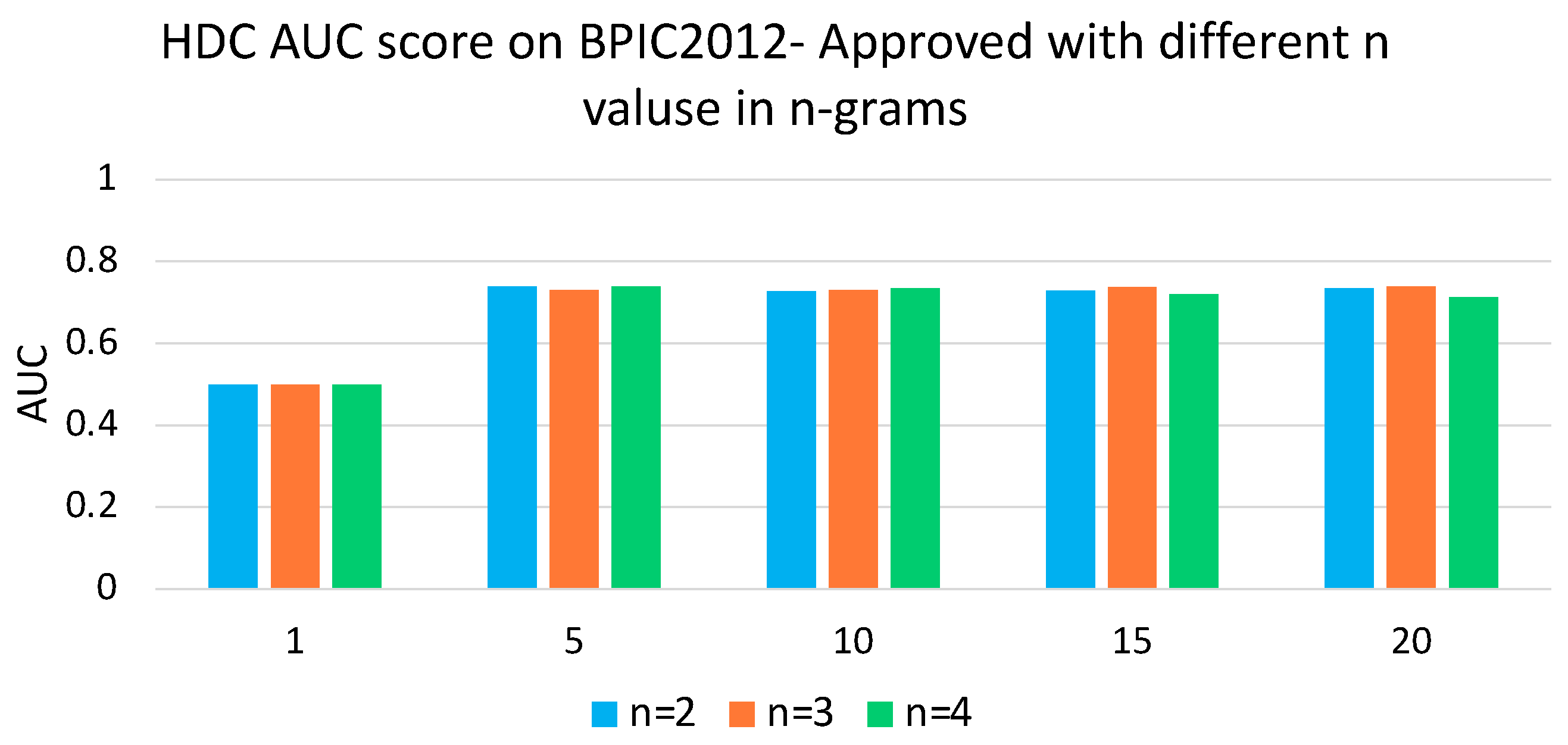
To analyze the impact of D dimensions in the encoding process, we experimented with different D values and did not observe significant changes across different datasets for the above metrics. Figure 2 shows the AUC score on BPIC-2012-Approved dataset for the HDC method. The reported AUC scores at each prefix are the average of 10 iterations. As depicted in Figure 2, there are no notable changes in the AUC scores across D = 4 k and D = 6 k dimensions; hence, we chose D = 4 k for efficiency. Also, to choose that value of n in n-gram encoding, we experimented with different values of n and no significant difference was observed across all datasets. We show the results for one dataset for clarity and brevity. Figure 4 depicts the AUC score of our proposed HDC method across several n values on the BPIC-2012-Approved dataset. We observed a similar pattern across all different datasets and depict the results for one dataset for clarity and brevity. We set n = 3 following common practice in the literature and based on our observations discussed earlier [30,47,48].
For comparison, we used XGBoost [19], RF [8], SVM [39], LR [19], and Att-bi-LSTM [10] for predictive process monitoring tasks, specifically, outcome prediction. We also used a variation of LSTM, i.e., Att-bi-LSTM [10] as it yields better performance for outcome prediction than the LSTM method often discussed in the recent literature [21].
AUC Score: Table 5 compares the AUC values for different algorithms across all 12 binary classification tasks in different datasets. Our proposed Att-HDC yields the highest AUC for 7 out of the 12 binary classification tasks. However, the next best algorithm yields a higher AUC for only two classification tasks while having a high standard deviation of AUC of 18% across different datasets (compared to Att-HDC’s 9%). This variability implies inconsistent performance and sub-optimal results in some datasets. The reported AUC represents the algorithms’ performance in precision and recall and its ability to discriminate between positive and negative instances. Machine learning methods are often not generalizable to all different applications, so the average performance is a good criterion for showing the performance of a model. Notably, our HDC-based method, excluding attributes, outperforms the best state-of-the-art algorithms: it achieves an average AUC that is 5% higher compared to the best baseline, XGBoost [19]. Att-HDC, which considers event attributes, further improves the AUC score, outperforming XGBoost [19], RF [8], SVM [39], LR [19], and Att-bi-LSTM [10] by an average of 6%, 6%, 6%, and 7.4%, respectively.
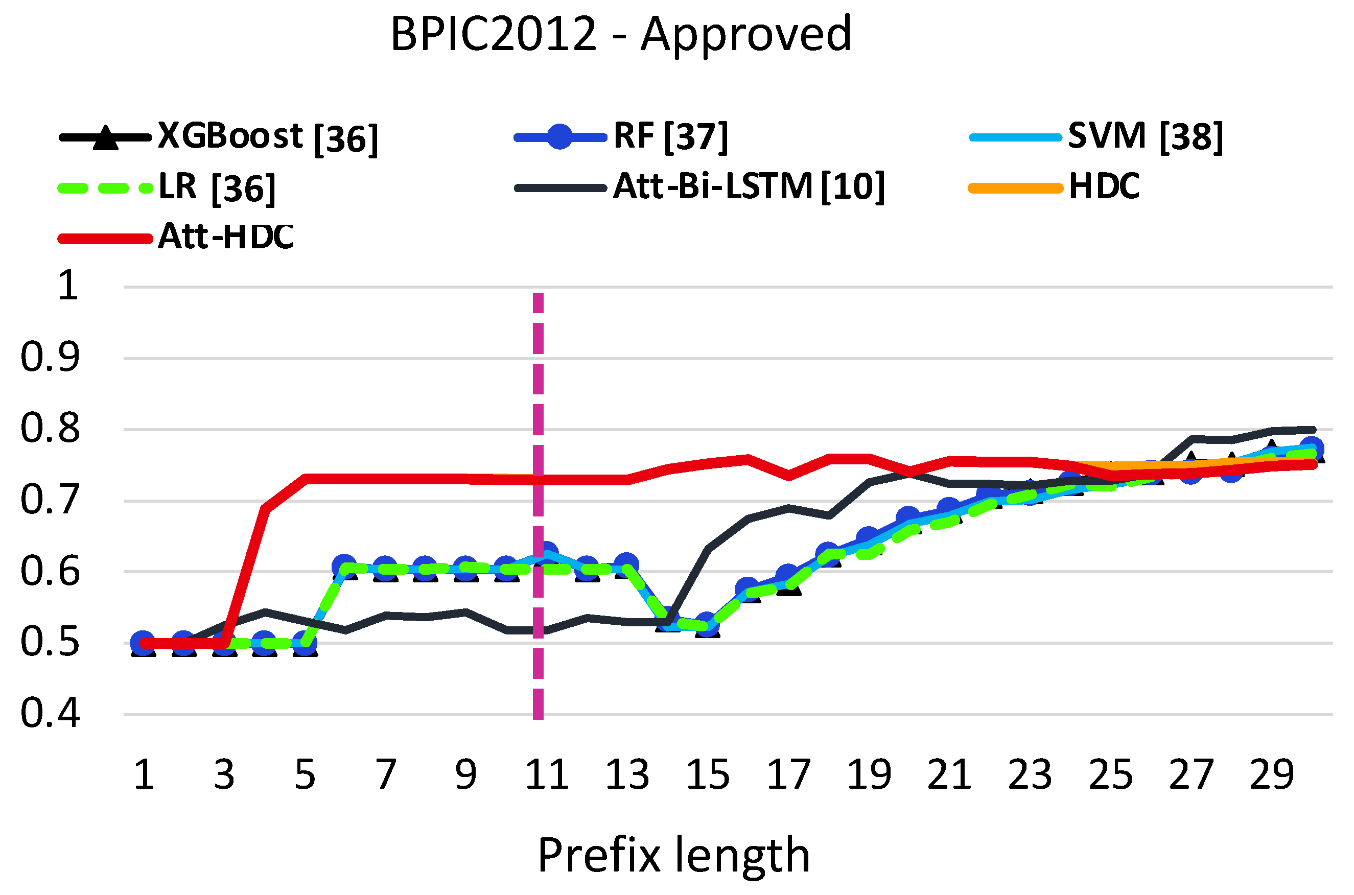
As an example, in Figure 5, we show the AUC scores of all the methods on prefixes of lengths 1 to 30 for the ‘ BPIC 2012 Approved ’ dataset. The vertical line at index 11 indicates the median length of the processes, i.e., half of the processes finish before they reach the 11th event in the process. Evidently, our proposed methods yield higher AUC scores, particularly in the early stages of processes, reaching an AUC score of 0.69 with only observing four events of processes on average. A similar AUC score is observed for both the Att-HDC and HDC methods, implying that adding event attributes in Att-HDC did not contribute to better distinguishing between positive and negative instances as intended using the AUC metric. For the other methods, it takes a longer time (and process length) to reach a comparable AUC score. For example, the best method Att-bi-LSTM [10] yields a similar AUC score to our proposed methods after observing 20 events in the traces. Therefore, Figure 5 implies that a better AUC score is gained in the early stages of an ongoing process, which ultimately leads to preserving memory and computation and enabling earlier corrective measures in business processes.
F1-Score: Table 6 reports the average F1-score values for the various prefix lengths from 3 to the median length of traces within each dataset with a step size of 3. The table contains the average F1-score of all the 12 classification tasks across four event logs. Our proposed methods yield higher F1-scores in 9 out of 12 classification tasks. Also, our proposed Att-HDC method yields an average F1-score of 76%, which is 6% higher in comparison to the best state-of-the-art approaches.
Earliness: Earliness measures how early a classifier predicts the terminating state in terms of event count [10]. We evaluate the earliness of our HDC-based and Att-HDC methods, along with state-of-the-art methods, across all event logs. Table 7 compares the earliness of the methods as a fraction of the whole sequence length, i.e., what fraction of the whole trace was needed to be observed in order to achieve the same results. For instance, for the BPIC2012-Approved dataset, XGBoost [18] requires 82% of the whole process to yield a high accuracy, while this value is less than a percent for our proposed methods. HDC-based and Att-HDC methods achieve substantially better earliness, up to a 20× faster average earliness for a reliable prediction compared to the baseline methods.
Execution Time: We also report the execution time of our algorithm for the run-time (encoding the test query and Inference) in Table 8 for the full prefix length. Based on Table 8, HDC requires a lower run-time in comparison to the best baseline algorithms, namely, XGBoost [19], RF [8], and Att-bi-LSTM [10]. The proposed HDC’s property in eliminating encoding the traces from scratch, which was mentioned as single-pass inference] before, helps in lowering the time consumption. More specifically, our HDC method requires a 10 12 × lower run-time on average in comparison to XGBoost, RF, and Att-bi-LSTM, as well as Att-HDC. Att-HDC slightly consumes more time than HDC for encoding the attributes, but still, it is 4.8 × faster than the best state-of-the-art approach. We conclude that HDC’s and Att-HDC’s inference, including the mapping of the input data, is significantly faster than that of the state-of-the-art methods. This highlights HDC’s superiority for business processes, where the real-time aspect is imperative, e.g., online shopping processes.

5.4. Instance Sampling

Due to extensive training and hyper-parameter tuning, machine learning techniques are computationally expensive, which limits their practical application in dynamic business environments [12]. The instance sampling of training data aims to improve the training speed of processes by reducing training set size while maintaining accuracy. However, these methods often require additional computations for choosing samples within the training that best represent the whole data, which can still hinder their efficiency in real- world applications.
Hyperdimensional Computing has proven to yield high performance when trained on small portions of training data [49]. We use this property to further show the efficiency of our proposed method, which impedes the use of instance selection methods. We show that with small proportions of the training data that are randomly chosen, with hte HDC-based method, we can gain high performance using Hyperdimensional Computing. The F1-score and AUC on the BPIC2012-Approved dataset are shown in in Figure 6 for different ratios of the training data for prefixes of length 11 (median length of traces in this dataset). We depict the results of one dataset for brevity. We consider the samples being chosen independently and randomly without replacement. The depicted results are the average, minimum, and maximum over 10 iterations. We observe a similar average F1-score and AUC score with a sampling ratio of 0.5 for the training data. As can be observed in Figure 6, the error bars are narrow, indicating that the inherent variability in the data has a minimal impact on the model’s performance metrics across different subsampling ratios, and the results are consistent with different iterations over the dataset. Figure 6 also shows that with a 10% of the training data, our proposed method still yields high performance (only 3% and 5.1% drops in average F1-score and AUC score in comparison to training on the whole data).
Our proposed method streamlines predictive training using a single-pass inference approach and leveraging known tri-grams, while other algorithms require repetitive encoding and training for each prefix. Preserving attributes alongside event patterns incurs slight latency for Att-HDC but significantly improves the F1-score by up to 14% and AUC by an average of 6%, and an average 20× faster earliness. The experiments were conducted using Python 3.8 on a computer with a 2.3 GHz quad-core Intel Core i5 and 8 GB of RAM.

6. Discussion of Limitations and Future Work

Process mining data during the execution of business processes can be generated and stored in noisy environments. Noise could come from human error in inputting information, environmental factors such as network interruptions, and other sources. Future research can investigate the reliability and robustness to noise of the predictive process monitoring methods. Also, this study paves the way to several other future work directions. Further analysis can be applied in choosing event attributes as in Section 4.6 rather than merely considering the frequency of the attributes. Also, adding trace attributes might help in distinguishing traces with different outcomes. As the next step, we aim to apply a novel retraining technique for weighted retraining as in Section 4.5. In weighted retraining, a higher value is assigned to infrequent historical traces to decrease the impact of dominant patterns in traces and further improve the prediction results. Also, recently, many studies have tried to use the benefits of both NN-based and HD-based methods, i.e., combining a feature extraction factor in NN-based methods with the energy efficiency and simplicity of Hyperdimensional Computing [49]. In the next step, rather than using the raw sequences, we aim to extract more useful spatiotemporal features from the data using neural network based methods for the better extraction of features and then deploy our method on the extracted features.

7. Conclusions

We proposed a novel approach based on HDC learning for predicting the outcome of ongoing processes. Unlike previous approaches, our technique builds upon preserving the pattern of events and event attributes in fixed-length vectors (disregarding prefix length) rather than using one-hot encoded vectors or frequency-based feature vectors. Also, our proposed method does not need conventional hyper-parameter tuning found in machine learning-based algorithms. Our algorithm stores the subsets (n-grams) of trace prefixes and maps the observed patterns into a high-dimensional space to realize a linearly separable classifier on historical data using basic element-wise operations along the vectors. Our experimental results on four publicly available event logs with a general of 12 classification tasks show the efficiency of the proposed method in improving the F1-score by up to 14% and average AUC scores by 6% in the early prefixes within an ongoing process. The average AUC and F1 scores across all prefix lengths are improved in our algorithm while yielding a comparable F1-score. Also, due to single-pass inference, our algorithm has up to 20× higher earliness in comparison to the best state-of-the art methods, i.e., our proposed methods yield high F1-scores and AUC scores in the initial observed events of the processes. Also, when observing 10% of the input data using our proposed methods only slightly affects the F1-score and AUC, meaning that less computation and memory overhead is needed. Based on our observations, patterns and order of events together with event attributes provide valuable insights about how a particular ongoing trace will end. Our proposed algorithm yields a more accurate prediction in the early steps of an ongoing process instance compared to other algorithms, and the earlier an accurate prediction is conducted, the more useful it will be in practice.

Author Contributions

Conceptualization, F.A. and A.T.; Methodology, F.A.; Software, F.A.; Validation, B.A.; Formal analysis, F.A.; Investigation, A.T., R.H. and Z.Z.; Writing—original draft, F.A.; Writing—review & editing, A.T., R.H., Z.Z., S.R., T.R. and B.A.; Supervision, A.T., S.R., T.R. and B.A.; Project administration, S.R., T.R. and B.A.; Funding acquisition, S.R., T.R. and B.A. All authors have read and agreed to the published version of the manuscript.

Funding

This work was supported in part by Center for Processing with Intelligent Storage and Memory (PRISM) #2023-JU-3135, CoCoSys, centers in JUMP 2.0, an SRC program sponsored by DARPA and, also NSF grants #1952225, #1952247, #2003279, #1826967, #1911095, #2052809, #2112665, and #2112167.

Data Availability Statement

The original data presented in the study are publicly available from the Business Process Intelligence Challenge (BPIC), widely used in the literature, BPIC 2012, BPIC 2015, BPIC 2017 and BPIC 2019.

Conflicts of Interest

The authors declare no conflict of interest.

References

  1. Teinemaa, I.; Dumas, M.; Rosa, M.L.; Maggi, F.M. Outcome-oriented predictive process monitoring: Review and benchmark. ACM Trans. Knowl. Discov. Data (TKDD) 2019, 13, 1–57. [Google Scholar] [CrossRef]
  2. van der Aalst, W.; Reijers, H.; Weijters, A.; van Dongen, B.; Alves de Medeiros, A.; Song, M.; Verbeek, H. Business process mining: An industrial application. Inf. Syst. 2007, 32, 713–732. [Google Scholar] [CrossRef]
  3. Márquez-Chamorro, A.E.; Resinas, M.; Ruiz-Cortés, A. Predictive monitoring of business processes: A survey. IEEE Trans. Serv. Comput. 2017, 11, 962–977. [Google Scholar] [CrossRef]
  4. Di Francescomarino, C.; Dumas, M.; Maggi, F.M.; Teinemaa, I. Clustering-based predictive process monitoring. IEEE Trans. Serv. Comput. 2016, 12, 896–909. [Google Scholar] [CrossRef]
  5. Evermann, J.; Rehse, J.R.; Fettke, P. A deep learning approach for predicting process behaviour at runtime. In Proceedings of the International Conference on Business Process Management, Rio de Janeiro, Brazil, 18–22 September 2016; Springer: Berlin/Heidelberg, Germany, 2016; pp. 327–338. [Google Scholar]
  6. Morariu, C.; Morariu, O.; Răileanu, S.; Borangiu, T. Machine learning for predictive scheduling and resource allocation in large scale manufacturing systems. Comput. Ind. 2020, 120, 103244. [Google Scholar] [CrossRef]
  7. Aalikhani, R.; Fathian, M.; Rasouli, M.R. Comparative Analysis of Classification-Based and Regression-Based Predictive Process Monitoring Models for Accurate and Time-Efficient Remaining Time Prediction. IEEE Access 2024, 12, 67063–67093. [Google Scholar] [CrossRef]
  8. Verenich, I.; Dumas, M.; Rosa, M.L.; Maggi, F.M.; Teinemaa, I. Survey and Cross-Benchmark Comparison of Remaining Time Prediction Methods in Business Process Monitoring. ACM Trans. Intell. Syst. Technol. 2019, 10, 1–34. [Google Scholar] [CrossRef]
  9. Maggi, F.M.; Di Francescomarino, C.; Dumas, M.; Ghidini, C. Predictive monitoring of business processes. In Proceedings of the International Conference on Advanced Information Systems Engineering, Thessaloniki, Greece, 16–20 June 2014; Springer: Berlin/Heidelberg, Germany, 2014; pp. 457–472. [Google Scholar]
  10. Wang, J.; Yu, D.; Liu, C.; Sun, X. Outcome-oriented predictive process monitoring with attention-based bidirectional LSTM neural networks. In Proceedings of the 2019 IEEE International Conference on Web Services (ICWS), Milan, Italy, 8–13 July 2019; IEEE: Piscataway, NJ, USA, 2019; pp. 360–367. [Google Scholar]
  11. Xing, Z.; Pei, J.; Keogh, E. A brief survey on sequence classification. ACM Sigkdd Explor. Newsl. 2010, 12, 40–48. [Google Scholar] [CrossRef]
  12. Fani Sani, M.; Vazifehdoostirani, M.; Park, G.; Pegoraro, M.; van Zelst, S.J.; van der Aalst, W.M. Performance-preserving event log sampling for predictive monitoring. J. Intell. Inf. Syst. 2023, 61, 53–82. [Google Scholar] [CrossRef]
  13. Weytjens, H.; De Weerdt, J. Learning uncertainty with artificial neural networks for predictive process monitoring. Appl. Soft Comput. 2022, 125, 109134. [Google Scholar] [CrossRef]
  14. Park, G.; Song, M. Optimizing Resource Allocation Based on Predictive Process Monitoring. IEEE Access 2023, 11, 38309–38323. [Google Scholar] [CrossRef]
  15. Leontjeva, A.; Conforti, R.; Di Francescomarino, C.; Dumas, M.; Maggi, F.M. Complex symbolic sequence encodings for predictive monitoring of business processes. In Proceedings of the Business Process Management: 13th International Conference, BPM 2015, Innsbruck, Austria, 31 August–3 September 2015; Proceedings 13. Springer: Berlin/Heidelberg, Germany, 2015; pp. 297–313. [Google Scholar]
  16. Ramirez-Alcocer, U.M.; Tello-Leal, E.; Romero, G.; Macías-Hernández, B.A. A Deep Learning Approach for Predictive Healthcare Process Monitoring. Information 2023, 14, 508. [Google Scholar] [CrossRef]
  17. De Leoni, M.; Van der Aalst, W.M.; Dees, M. A general framework for correlating business process characteristics. In Proceedings of the International Conference on Business Process Management, Haifa, Israel, 7–11 September 2014; Springer: Berlin/Heidelberg, Germany, 2014; pp. 250–266. [Google Scholar]
  18. Vazifehdoostirani, M.; Abbaspour Onari, M.; Grau, I.; Genga, L.; Dijkman, R. Uncovering the Hidden Significance of Activities Location in Predictive Process Monitoring. In Proceedings of the International Conference on Process Mining, Rome, Italy, 23–27 October 2023; Springer: Berlin/Heidelberg, Germany, 2023; pp. 191–203. [Google Scholar]
  19. El-Khawaga, G.; Abu-Elkheir, M.; Reichert, M. Xai in the context of predictive process monitoring: An empirical analysis framework. Algorithms 2022, 15, 199. [Google Scholar] [CrossRef]
  20. Camargo, M.; Dumas, M.; González-Rojas, O. Learning accurate LSTM models of business processes. In Proceedings of the International Conference on Business Process Management, Vienna, Austria, 1–6 September 2019; Springer: Berlin/Heidelberg, Germany, 2019; pp. 286–302. [Google Scholar]
  21. De Smedt, J.; De Weerdt, J. Predictive process model monitoring using long short-term memory networks. Eng. Appl. Artif. Intell. 2024, 133, 108295. [Google Scholar] [CrossRef]
  22. Kim, S.; Comuzzi, M.; Di Francescomarino, C. Understanding the Impact of Design Choices on the Performance of Predictive Process Monitoring. In Proceedings of the International Conference on Process Mining, Rome, Italy, 23–27 October 2023; Springer: Berlin/Heidelberg, Germany, 2023; pp. 153–164. [Google Scholar]
  23. Kanerva, P. Hyperdimensional computing: An introduction to computing in distributed representation with high-dimensional random vectors. Cogn. Comput. 2009, 1, 139–159. [Google Scholar] [CrossRef]
  24. Thomas, A.; Dasgupta, S.; Rosing, T. Theoretical Foundations of Hyperdimensional Computing. J. Artif. Intell. Res. 2021, 72, 215–249. [Google Scholar] [CrossRef]
  25. Van Der Aalst, W. Process mining. Commun. ACM 2012, 55, 76–83. [Google Scholar] [CrossRef]
  26. Vidgof, M.; Wurm, B.; Mendling, J. The Impact of Process Complexity on Process Performance: A Study using Event Log Data. In Proceedings of the International Conference on Business Process Management, Utrecht, The Netherlands, 11–15 September 2023; Springer: Berlin/Heidelberg, Germany, 2023; pp. 413–429. [Google Scholar]
  27. Thapa, R.; Lamichhane, B.; Ma, D.; Jiao, X. Spamhd: Memory-efficient text spam detection using brain-inspired hyperdimensional computing. In Proceedings of the 2021 IEEE Computer Society Annual Symposium on VLSI (ISVLSI), Tampa, FL, USA, 7–9 July 2021; IEEE: Piscataway, NJ, USA, 2021; pp. 84–89. [Google Scholar]
  28. Imani, M.; Nassar, T.; Rahimi, A.; Rosing, T. Hdna: Energy-efficient dna sequencing using hyperdimensional computing. In Proceedings of the 2018 IEEE EMBS International Conference on Biomedical & Health Informatics (BHI), Las Vegas, NV, USA, 4–7 March 2018; IEEE: Piscataway, NJ, USA, 2018; pp. 271–274. [Google Scholar]
  29. Watkinson, N.; Givargis, T.; Joe, V.; Nicolau, A.; Veidenbaum, A. Class-modeling of septic shock with hyperdimensional computing. In Proceedings of the 2021 43rd Annual International Conference of the IEEE Engineering in Medicine & Biology Society (EMBC), Virtual, 1–5 November 2021; IEEE: Piscataway, NJ, USA, 2021; pp. 1653–1659. [Google Scholar]
  30. Ge, L.; Parhi, K.K. Classification using hyperdimensional computing: A review. IEEE Circuits Syst. Mag. 2020, 20, 30–47. [Google Scholar] [CrossRef]
  31. Rahimi, A.; Benatti, S.; Kanerva, P.; Benini, L.; Rabaey, J.M. Hyperdimensional biosignal processing: A case study for EMG-based hand gesture recognition. In Proceedings of the 2016 IEEE International Conference on Rebooting Computing (ICRC), San Diego, CA, USA, 17–19 October 2016; IEEE: Piscataway, NJ, USA, 2016; pp. 1–8. [Google Scholar]
  32. Khaleghi, B.; Xu, H.; Morris, J.; Rosing, T.Š. tiny-hd: Ultra-efficient hyperdimensional computing engine for iot applications. In Proceedings of the 2021 Design, Automation & Test in Europe Conference & Exhibition (DATE), Grenoble, France, 1–5 February 2021; IEEE: Piscataway, NJ, USA, 2021; pp. 408–413. [Google Scholar]
  33. Akiba, T.; Sano, S.; Yanase, T.; Ohta, T.; Koyama, M. Optuna: A next-generation hyperparameter optimization framework. In Proceedings of the 25th ACM SIGKDD International Conference on Knowledge Discovery & Data Mining, Anchorage, AK, USA, 4–8 August 2019; pp. 2623–2631. [Google Scholar]
  34. Asgarinejad, F.; Morris, J.; Rosing, T.; Aksanli, B. PIONEER: Highly Efficient and Accurate Hyperdimensional Computing using Learned Projection. In Proceedings of the 2024 29th Asia and South Pacific Design Automation Conference (ASP-DAC), Incheon, Republic of Korea, 22–25 January 2024; IEEE: Piscataway, NJ, USA, 2024; pp. 896–901. [Google Scholar]
  35. Pale, U.; Teijeiro, T.; Rheims, S.; Ryvlin, P.; Atienza, D. Combining general and personal models for epilepsy detection with hyperdimensional computing. Artif. Intell. Med. 2024, 148, 102754. [Google Scholar] [CrossRef]
  36. Nunes, I.; Heddes, M.; Givargis, T.; Nicolau, A.; Veidenbaum, A. GraphHD: Efficient graph classification using hyperdimensional computing. In Proceedings of the 2022 Design, Automation & Test in Europe Conference & Exhibition (DATE), Antwerp, Belgium, 14–23 March 2022; IEEE: Piscataway, NJ, USA, 2022; pp. 1485–1490. [Google Scholar]
  37. Hernández-Cano, A.; Zhuo, C.; Yin, X.; Imani, M. Reghd: Robust and efficient regression in hyper-dimensional learning system. In Proceedings of the 2021 58th ACM/IEEE Design Automation Conference (DAC), San Francisco, CA, USA, 5–9 December 2021; IEEE: Piscataway, NJ, USA, 2021; pp. 7–12. [Google Scholar]
  38. Ge, L.; Parhi, K.K. Robust clustering using hyperdimensional computing. IEEE Open J. Circuits Syst. 2024, 5, 102–116. [Google Scholar] [CrossRef]
  39. Kratsch, W.; Manderscheid, J.; Röglinger, M.; Seyfried, J. Machine learning in business process monitoring: A comparison of deep learning and classical approaches used for outcome prediction. Bus. Inf. Syst. Eng. 2021, 63, 261–276. [Google Scholar] [CrossRef]
  40. Di Francescomarino, C.; Ghidini, C.; Maggi, F.M.; Milani, F. Predictive process monitoring methods: Which one suits me best? In Proceedings of the International Conference on Business Process Management, Sydney, Australia, 9–14 September 2018; Springer: Berlin/Heidelberg, Germany, 2018; pp. 462–479. [Google Scholar]
  41. Rahimi, A.; Kanerva, P.; Rabaey, J.M. A robust and energy-efficient classifier using brain-inspired hyperdimensional computing. In Proceedings of the 2016 International Symposium on Low Power Electronics and Design, San Francisco, CA, USA, 8–10 August 2016; pp. 64–69. [Google Scholar]
  42. Ma, D.; Hao, C.; Jiao, X. Hyperdimensional computing vs. neural networks: Comparing architecture and learning process. In Proceedings of the 2024 25th International Symposium on Quality Electronic Design (ISQED), San Francisco, CA, USA, 3–5 April 2024; IEEE: Piscataway, NJ, USA, 2024; pp. 1–5. [Google Scholar]
  43. Kononenko, I.; Kukar, M. Machine Learning and Data Mining; Horwood Publishing: Chichester, UK, 2007. [Google Scholar]
  44. Bradley, A.P. The use of the area under the ROC curve in the evaluation of machine learning algorithms. Pattern Recognit. 1997, 30, 1145–1159. [Google Scholar] [CrossRef]
  45. Drodt, C.; Weinzierl, S.; Matzner, M.; Delfmann, P. Predictive Recommining: Learning Relations between Event Log Characteristics and Machine Learning Approaches for Supporting Predictive Process Monitoring. In Proceedings of the International Conference on Advanced Information Systems Engineering, Zaragoza, Spain, 12–16 June 2023; Springer: Berlin/Heidelberg, Germany, 2023; pp. 69–76. [Google Scholar]
  46. Alonso, P.; Shridhar, K.; Kleyko, D.; Osipov, E.; Liwicki, M. HyperEmbed: Tradeoffs between resources and performance in NLP tasks with hyperdimensional computing enabled embedding of n-gram statistics. In Proceedings of the 2021 International Joint Conference on Neural Networks (IJCNN), Shenzhen, China, 18–22 July 2021; IEEE: Piscataway, NJ, USA, 2021; pp. 1–9. [Google Scholar]
  47. Kanerva, P. Hyperdimensional computing: An algebra for computing with vectors. Advances in Semiconductor Technologies: Selected Topics Beyond Conventional CMOS; John Wiley & Sons: Hoboken, NJ, USA, 2022; pp. 25–42. [Google Scholar]
  48. Najafabadi, F.R.; Rahimi, A.; Kanerva, P.; Rabaey, J.M. Hyperdimensional computing for text classification. In Proceedings of the Design, Automation Test in Europe Conference Exhibition (DATE), Dresden, Germany, 14–18 March 2016; p. 1. [Google Scholar]
  49. Rosato, A.; Panella, M.; Kleyko, D. Hyperdimensional computing for efficient distributed classification with randomized neural networks. In Proceedings of the 2021 International Joint Conference on Neural Networks (IJCNN), Shenzhen, China, 18–22 July 2021; IEEE: Piscataway, NJ, USA, 2021; pp. 1–10. [Google Scholar]
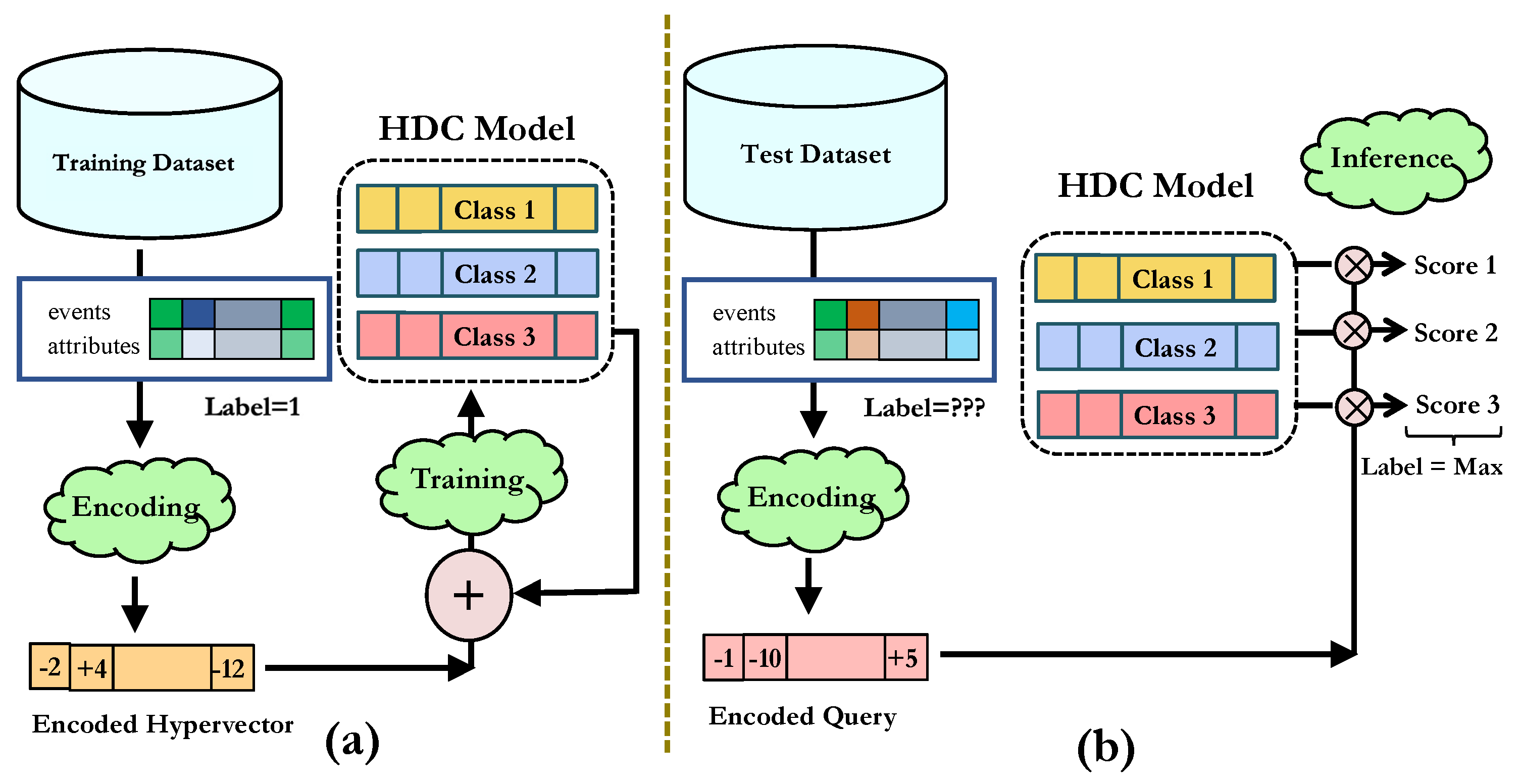
Figure 1. (a) HDC encoding and training. Each training data point (business process sequence) is encoded to a hypervector, and then in the training phase, it is added up to the proper class hypervector based on its label. This operation is a simple element-wise addition. In (b), HDC Inference, a business process query sequence is similarly encoded and compared with all the class hypervectors. The index of the class with the highest similarity is returned as a prediction result.
Information 15 00490 g001
Figure 2. AUC score over different prefixes (process lengths) for BPIC2012—Approved dataset with different D values.
Information 15 00490 g002
Figure 3. Proposed HDC framework steps: encoding, which includes (1) projecting unique event IDs and unique attributes into hypervectors and (2) binding attributes’ hypervectors to the events, encoding tri-grams, and superimposing for generating the hypervector corresponding to each input trace; training (3), wherein class hypervectors are generated with the element-wise summation of elements belonging to the class; querying (4), where the label of a query data is predicted using a similarity metric; and (5) retraining, which includes updating class vectors based on the correct/incorrect label prediction of the query data.
Information 15 00490 g003
Figure 4. AUC score over different prefixes (process lengths) for BPIC2012—Approved dataset with different n values in n—gram encoding.
Information 15 00490 g004
Figure 5. AUC score over different prefixes (process lengths) for BPIC2012—Approved dataset for different methods. Red and orange curves, respectively, depict Att-HDC and HDC, which yield higher AUCs in early prefixes of traces.
Information 15 00490 g005
Figure 6. AUC and F1-score for various training data ratios on the BPIC2012-Approved dataset.
Information 15 00490 g006
Table 1. BPIC—2019 event log traces.
Trace IDEvent NameTimestampResource and UserCumulative Net Worth (EUR)
trace 338Create Purchase Order Item2018-01-02T03:20:00.000Zbatch-041833.0
Record Goods Receipt2018-01-22T16:33:00.000Zuser-0311833.0
Vendor creates invoice2018-01-25T22:59:00.000ZNONE1833.0
Record Invoice Receipt2018-02-02T12:28:00.000Zuser-0071833.0
Clear Invoice2018-02-22T15:17:00.000Zuser-0021833.0
trace 529Create Purchase Order Item2018-01-02T08:51:00.000Zuser-0520.0
Record Goods Receipt2018-01-18T10:02:00.000Zuser-0530.0
trace 198181Create Purchase Order Item2018-10-15T05:34:00.000Zuser-11915.0
Record Goods Receipt2018-10-18T11:43:00.000Zuser-08015.0
Create Purchase Order Item2018-10-24T21:59:00.000ZNONE15.0
Clear Invoice2018-11-15T14:35:00.000Zuser-00215.0
Table 2. HDC application and performance in different domains.
Application DomainTask & ReferenceDataset Type/NamePerformance
Image ClassificationClassification [34]Images (CIFAR10, MNIST, etc.)Increased accuracy/energy efficiency vs. SOTA
GenomicsClassification [28]DNA sequencesIncreased accuracy/lower time and energy vs. SOTA
Graph AnalyticsClassification [36]GraphsFaster inference vs. SOTA
Economics and EnergyRegression [37]Boston housing, CCPP, etc.Faster and energy efficient vs. SOTA
BioinformaticsClustering [38]IRIS, ISOLET, RNA-seq, etc.Higher clustering accuracy/less execution time vs. SOTA
Table 3. Table of notations.
SymbolDefinitionSymbolDefinition
D dimension of encoded data H hypervector of encoded data
L level hypervector { ± 1 } D P n permutation by n indexes
eeventCclass hypervector
ttrace ω tri-gram of events
λ trace prefix a t t r event attribute
mtrace lengthQ# of quantized levels
e k prediction eventlquantizer’s level hypervector { ± 1 } D
Table 4. Statistics of benchmark event logs.
DatasetTracesMin LenMedian LenMax LenUnique EventsEvent Attr.Pos. Class Ratio
BPIC 12 Approved 13,0873111752430.19
BPIC 12 Cancelled 13,0873111752430.22
BPIC 12 Declined 13,0873111752430.58
BPIC 15 1 119924410128900.24
BPIC 15 2 83215413230400.19
BPIC 15 3 140934212427700.20
BPIC 15 4 105314411627200.16
BPIC 15 5 115655015428500.31
BPIC 17 Approved 31,41310351802640.41
BPIC 17 Cancelled 31,41310351802640.12
BPIC 17 Declined 31,41310351802640.47
BPIC 19 251,734159904230.72
Table 5. Comparison of average and std of AUC in early prefixes (before median length).
Baseline MethodsProposed MethodsBest HDC-Based vs.
Best Baseline (%)
DatasetXGBoost [19]RF [1]SVM [39]LR [1]Att-bi-LSTM [10]HDCAtt-HDC
BPIC 2012 Approved 0.56 ± 0.060.56 ± 0.060.56 ± 0.060.56 ± 0.050.52 ± 0.020.66 ± 0.010.66 ± 0.01+10%
BPIC 2012 Cancelled 0.57 ± 0.080.57 ± 0.080.57 ± 0.080.57 ± 0.080.58 ± 0.090.66 ± 0.010.66 ± 0.01+8%
BPIC 2012 Declined 0.81 ± 0.150.81 ± 0.150.81 ± 0.160.81 ± 0.150.74 ± 0.170.73 ± 0.140.70 ± 0.13−8%
BPIC 2015 1 0.80 ± 0.170.82 ± 0.160.81 ± 0.160.82 ± 0.160.77 ± 0.140.85 ± 0.140.85 ± 0.14+3%
BPIC 2015 2 0.81 ± 0.170.81 ± 0.160.81 ± 0.110.82 ± 0.140.73 ± 0.200.82 ± 0.110.82 ± 0.110%
BPIC 2015 3 0.80 ± 0.170.81 ± 0.160.81 ± 0.120.83 ± 0.150.71 ± 0.180.86 ± 0.140.86 ± 0.14+3%
BPIC 2015 4 0.60 ± 0.380.57 ± 0.410.44 ± 0.380.46 ± 0.370.59 ± 0.340.85 ± 0.230.85 ± 0.23+23%
BPIC 2015 5 0.83 ± 0.140.81 ± 0.160.86 ± 0.110.83 ± 0.140.78 ± 0.150.82 ± 0.150.82 ± 0.15−1%
BPIC 2017 Approved 0.65 ± 0.120.52 ± 0.050.66 ± 0.130.65 ± 0.120.84 ± 0.150.59 ± 0.080.60 ± 0.11−24%
BPIC 2017 Cancelled 0.68 ± 0.150.69 ± 0.150.68 ± 0.150.66 ± 0.140.69 ± 0.150.67 ± 0.130.71 ± 0.14+2%
BPIC 2017 Declined 0.70 ± 0.150.70 ± 0.140.69 ± 0.150.68 ± 0.150.67 ± 0.140.74 ± 0.110.75 ± 0.13+ 5%
Average 0.70 ± 0.180.70 ± 0.090.70 ± 0.140.70 ± 0.240.69 ± 0.150.75 ± 0.090.76 ± 0.09 + 6 %
Table 6. Comparison of average and std of F1-score in early prefixes (before median length).
Baseline MethodsProposed MethodsBest HDC-Based vs.
Best Baseline (%)
DatasetXGBoost [19]RF [1]SVM [39]LR [1]Att-bi-LSTM [10]HDCAtt-HDC
BPIC 2012 Approved 0.53 ± 0.100.55 ± 0.090.53 ± 0.100.53 ± 0.140.53 ± 0.090.55 ± 0.190.60 ± 0.12+7%
BPIC 2012 Cancelled 0.54 ± 0.120.54 ± 0.120.54 ± 0.110.55 ± 0.120.53 ± 0.120.59 ± 0.110.59 ± 0.11+4%
BPIC 2012 Declined 0.82 ± 0.150.78 ± 0.210.78 ± 0.210.78 ± 0.200.77 ± 0.190.67 ± 0.230.69 ± 0.23−14%
BPIC 2015 1 0.73 ± 0.230.74 ± 0.230.68 ± 0.220.70 ± 0.270.66 ± 0.130.76 ± 0.170.76 ± 0.17+2%
BPIC 2015 2 0.74 ± 0.210.76 ± 0.230.73 ± 0.180.77 ± 0.220.69 ± 0.110.73 ± 0.160.73 ± 0.16−3%
BPIC 2015 3 0.76 ± 0.220.76 ± 0.220.73 ± 0.180.77 ± 0.220.69 ± 0.160.79 ± 0.150.79 ± 0.15+2%
BPIC 2015 4 0.75 ± 0.220.76 ± 0.220.72 ± 0.170.76 ± 0.210.71 ± 0.180.73 ± 0.190.73 ± 0.19−3%
BPIC 2015 5 0.64 ± 0.070.65 ± 0.060.65 ± 0.060.72 ± 0.260.63 ± 0.080.73 ± 0.050.73 ± 0.05+7%
BPIC 2017 Approved 0.63 ± 0.130.50 ± 0.070.63 ± 0.130.63 ± 0.140.73 ± 0.160.63 ± 0.090.67 ± 0.11+4%
BPIC 2017 Cancelled 0.67 ± 0.160.67 ± 0.160.66 ± 0.160.67 ± 0.160.67 ± 0.160.63 ± 0.130.67 ± 0.140%
BPIC 2017 Declined 0.52 ± 0.090.53 ± 0.100.52 ± 0.100.52 ± 0.090.52 ± 0.090.56 ± 0.060.58 ± 0.06+3%
Average 0.52 ± 0.090.53 ± 0.100.52 ± 0.100.52 ± 0.090.52 ± 0.090.56 ± 0.060.58 ± 0.06 + 6 %
Table 7. Comparison of average earliness (as a fraction of the whole trace) in different processes within an event log.
Baseline MethodsProposed Methods
DatasetXGBoost [19]RF [8]SVM [39]LR [19]Att-bi-LSTM [10]HDC-BasedAtt-HDC
BPIC 2012 Approved 0.820.820.820.820.820.0490.049
BPIC 2012 Cancelled 1.001.001.001.001.000.0510.051
BPIC 2012 Declined 0.790.790.790.790.790.0270.027
BPIC 2015 1 0.800.820.780.820.820.0210.021
BPIC 2015 2 0.800.820.780.820.820.0210.021
BPIC 2015 3 0.800.820.780.820.820.0210.021
BPIC 2015 4 0.800.820.780.820.820.0210.021
BPIC 2015 5 0.800.820.780.820.820.0210.021
BPIC 2017 Approved 0.790.790.790.790.790.0270.027
BPIC 2017 Cancelled 0.780.780.780.780.780.0280.028
BPIC 2017 Declined 0.790.791.00.790.790.0200.020
Table 8. Algorithms’ overall average run-times (s) in event logs (over all prefixes).
DatasetRFXGBoostAtt-bi-LSTMHDCAtt-HDC
BPIC2012—Approved107147110.6113
BPIC2012—Cancelled12912370.4716
BPIC2012—Declined2369880.4817
BPIC2015—1211011080.160.16
BPIC2015—236422170.110.11
BPIC2015—329331340.50.5
BPIC2015—43028980.360.36
BPIC2015—533171240.628
BPIC2017—Approved1431122171436
BPIC2017—Cancelled204183187529
BPIC2017—Declined1811542191135
BPIC2019153249104104139
Average107.08114.08128.5810.3826.35
Disclaimer/Publisher’s Note: The statements, opinions and data contained in all publications are solely those of the individual author(s) and contributor(s) and not of MDPI and/or the editor(s). MDPI and/or the editor(s) disclaim responsibility for any injury to people or property resulting from any ideas, methods, instructions or products referred to in the content.