1. Introduction
The explosion of big data has enabled solutions for many complex problems. Different approaches using mathematical simulation and relevant ideas, such as artificial intelligence [
1], the enhancement of computer capacity, and the use of super calculators, have made handling big data an easier task [
2]. The enhancement of these technologies is necessary due to the continuous amount of data generated by humans every second. Traditional programming is not efficient for fixing data mining problems [
3]. So, the idea of making computers function like the human brain, which learns from its tasks and makes complex decisions, has impacted our approach to the most challenging problems.
Likewise, these technologies have impacted global business [
4]. Different financial institutions and banks have endeavored to improve the services they provide to their customers by developing more sophisticated payment systems and ensuring the secure transfer of large amounts of money [
5]. Blockchain, artificial intelligence, big data, and other technologies have been successfully implemented into production in these network systems [
6]. However, fraudulent payments involving credit cards have evolved to a more advanced level [
7].
The COVID-19 pandemic is one of the most challenging problems for humanity. Countries have made significant progress in combating this disease. During this time, companies have successfully digitalized their businesses and streamlined their systems for users [
8]. Credit cards have become the first method of payment on e-commerce websites [
9]. In contrast, criminals try to breach these payment systems to make illegal transactions; thus, security is essential in these systems. Many solutions for addressing this problem have been proposed, several of which use the abilities of machine learning algorithms for classifying fraudulent transactions based on historical datasets [
10].
Every payment system for credit card transactions comprises four components: the merchant, cardholder, acquiring bank, and issuing bank. These four components communicate with each other using HTTP requests to make the transaction possible [
11]. The transaction is handled and checked differently by the issuing bank. Their main objective is to confirm that the transaction is legitimate. This system can be described as follows. First, the cardholder presents their credit card to the merchant for the purchase of goods or services. Then, the card is swiped and entered into the point-of-sale software, and the processor sends out a request for authorization through the payment processing networks [
12]. The issuing bank authorizes or rejects the transaction based on the funds available. After that, if the transaction is authorized, it is passed through the electronic networks to the processor, and the approval code is delivered to the point-of-sale device at the merchant’s location [
13]. The issuing bank then sends the money to the processing company to reimburse them for the purchase that was made. This whole process is completed in a matter of seconds.
Figure 1 illustrates these steps in detail.
This paper introduces an innovative adaptive credit card fraud detection system, leveraging three robust deep learning architectures alongside the Bayesian optimization algorithm. Its goal is to allow the selection of the most effective architecture for fraudulent transaction classification. A key contribution of this work lies in adapting the Bayesian optimization approach to efficiently navigate the complex landscape of deep learning model architectures. Unlike traditional methods such as grid search or random search, Bayesian optimization addresses the computational challenges and exponential complexity inherent in deep learning models, offering a more effective search mechanism. The system’s performance is evaluated using three distinct scenarios, where the Bayesian algorithm is fine-tuned across 50, 70, and 100 iterations, respectively, and the European credit card dataset is utilized for benchmarking. Furthermore, a comprehensive set of evaluation metrics is proposed to assess the performance of deep learning architectures with hyperparameter optimization using the Bayesian technique. This work significantly advances credit card fraud detection by presenting a holistic approach that integrates advanced techniques to achieve superior accuracy and efficiency in identifying fraudulent transactions.
This work makes the following contributions:
A hyperparameter tuning technique based on Bayesian optimization is proposed for selecting the best-performing deep learning architecture.
Bayesian optimization is implemented for designing the best-performing deep learning architectures, including RNN, LSTM, and ANN.
Several experiments based on the European credit card dataset are performed, and the obtained results show that the RNN is the most efficient with Bayesian hyperparameter optimization compared to the LSTM and ANN techniques.
The rest of this paper is organized as follows.
Section 2 provides a review of the literature.
Section 3 describes the methods used in this study.
Section 4 presents the proposed methodology and materials. The results and discussion are presented in
Section 5. Finally, in
Section 6 we present our conclusions and a brief description of our future work.
2. Related Works
The detection of illegal transactions has received much attention in the past decade. This has resulted from the number of transactions made by cardholders and the advanced approaches used by criminals to hack credit card information using techniques such as site duplication. In this section, we review some important works on the detection of fraudulent transactions using various techniques, such as machine learning and deep learning, as well as different approaches for enhancing these models, such as feature engineering, hyperparameter optimization, feature selection, and so on.
In [
14], the authors implemented a new solution for fraud transaction detection that was deployed in Apache Spark for real-time fraud identification. This solution used the following technologies: Kafka for programming tasks, Cassandra for dataset management, and Spark for real-time preprocessing and training. This solution was subjected to many experiments, to show its scalability and efficiency. Therefore, the paper introduces a novel fraud detection solution leveraging Apache Spark, Kafka, and Cassandra for real-time processing, demonstrating scalability and efficiency. Nonetheless, integrating multiple technologies may introduce complexity, while the system’s adaptability to evolving fraud tactics requires further examination. Another solution, presented in [
15], exploits several data mining techniques. Its main idea is to use a contrast vector for each transaction based on its cardholder’s historical behavior sequence. Then they profile the distinguishing ratio between the current transaction and the cardholder’s preferred behavior. After that, they used ContrastMiner, an algorithm implemented for discovering hidden patterns and differentiating fraudulent from non-fraudulent behavior. This was followed by combining predictions from different models and selecting the most effective pattern. Experiments conducted on real online banking data demonstrate that this solution yields significantly higher accuracy and lower alert volumes compared to the latest benchmark fraud detection system. The latter incorporates domain knowledge and traditional fraud detection methods. However, the utilization of ContrastMiner can be regarded as a potent approach for mitigating interpretability issues. Numerous experiments with extensive real online banking data have demonstrated its superiority in accuracy and reduction in alert volumes compared to conventional fraud detection methods, suggesting promising advancements in fraud detection efficiency.
Likewise, various deep learning architectures are successfully implemented for fraud transaction detection. They show efficient results in handling fraud transactions in many credit card datasets used for computation. For example, ref. [
16] invented a new approach for identifying fraudulent transactions. For this solution to detect fraud, hierarchical cluster-based deep neural networks (HC-DNNs) utilize anomaly characteristics pre-trained through an autoencoder as initial weights for deep neural networks. Through cross-validation, this method detected fraud more efficiently than conventional methods. In addition, the suggested solution can help discover the relationship between fraud types. Otherwise, mobile transactions are becoming more popular due to the increase in the number of smartphones that are attacked by fraudsters. Thus, securing those systems for payment is crucial. That is why our research introduces a novel approach for fraud detection using hierarchical cluster-based deep neural networks (HC-DNNs), leveraging anomaly characteristics pre-trained via autoencoder as initial weights. Despite its superior performance demonstrated through cross-validation, limitations arise with the growing prevalence of mobile transactions prone to fraud attacks, necessitating enhanced security measures to safeguard payment systems. The supervised machine learning algorithm XGBboost classifier [
17] is used to propose a solution [
18]. The obtained results demonstrate the strength of this solution.
Similarly, another solution occurs in [
19]. It detects credit card fraud transactions via employing 13 machine learning classifiers and a real credit card dataset. Their idea was to generate aggregated features using the genetic algorithm technique. Those generated features were compared with the original feature, as the best representative feature for identifying fraudulent transactions. As a result, based on many experiments, the aggregated features are more representative and efficient in identifying fraudulent transactions. The approach in this article presents a promising solution by combining multiple models. It generates aggregated features using the genetic algorithm technique. Despite yielding promising outcomes in various experiments, potential limitations may arise from dataset quality and scalability concerns, necessitating further investigation to assess real-world applicability accurately. In [
20], the authors proposed an efficient credit card fraud transaction solution based on representational learning. This solution implemented an innovative network architecture via an efficient inductive pooling operator and a careful downstream classifier. Several experiments conducted on a real credit card dataset demonstrated the outperformance of the proposed solution against the state-of-the-art methods. Generally, this introduces a credit card fraud detection solution using representational learning, showcasing superior performance via innovative network architecture. While promising, scalability challenges and the solution’s adaptability to evolving fraud tactics require further scrutiny for real-world efficacy.
In [
21], the authors implemented an intelligent credit card fraud transaction detection system. They implemented an aggregation strategy to classify fraudulent transactions. Its mechanism was to aggregate transactions to capture the cardholder’s period behavior and use them for model estimation. This solution is benchmarked on a real credit card dataset, and it shows higher performance in stopping abnormal transactions. Furthermore, the authors proposed a credit card fraud transaction detection method based on hyperparameter optimization [
22]. They used a differential evolution algorithm for selecting the performing hyperparameters of the XGboost algorithm. They benchmarked their solution with state-of-the-art classifiers. As a result, the proposed solution is efficient in distinguishing between fraud and non-fraud transactions. However, the solution’s scalability and adaptability to emerging fraud tactics necessitate further examination for practical deployment.
Unlike the cited solutions, our research introduces an adaptive system capable of effectively combating fraudulent transactions. By leveraging optimization techniques and exploiting the power of various deep learning architectures such as RNN, ANN, and LSTM, our approach aims to uncover hidden patterns within the dataset, facilitating the classification of fraudulent from non-fraudulent transactions. Notably, we employ Bayesian optimization as our main method for selecting the best architecture, addressing the complexity of deep learning models and resource-intensive computations. This method stands out for its effectiveness in adjusting hyperparameters and effectively exploring the search space.
6. Results and Discussion
The imbalanced European credit card dataset was transformed into a balanced dataset. This happened after removing several normal transactions from the majority class to test the three deep learning architectures with hyperparameter optimization using the Bayesian optimization approach. The random undersampling method with a sampling strategy is equal to 0.5. Moreover, the Bayesian optimization technique was used to design deep learning classifiers to improve the detection of fraudulent transactions. Several experiments were conducted with different numbers of iterations: 50, 70, and 100.
Table 3,
Table 4 and
Table 5 present the performance metrics and execution times of three deep learning models ANN, LSTM, and RNN. For 50 iterations, the ANN model achieved an accuracy (ACC) of 0.8939, with perfect precision (PER) and a geometric mean (GM) of 0.8024. However, its sensitivity (SEN) was relatively low at 0.6439 compared to LSTM and RNN. The RNN model demonstrated the highest ACC and AUC (0.9593 and 0.9767, respectively) among all models. As the number of iterations increased to 70 and 100, all models showed improvements in ACC, PER, GM, and AUC. Particularly, the LSTM model consistently exhibited high performance across all metrics, with ACC exceeding 0.95 in both 70 and 100 iterations. In terms of execution time, the LSTM model consistently took longest, followed by RNN and ANN. However, the execution time increased with the number of iterations for all models, indicating a trade-off between computational resources and model performance. Overall, the results suggest that LSTM outperformed ANN and RNN in terms of both performance metrics and computational efficiency for credit card fraud detection. However, further analysis considering other factors such as interpretability and scalability is necessary to determine the most suitable model for real-world deployment in fraud detection systems.
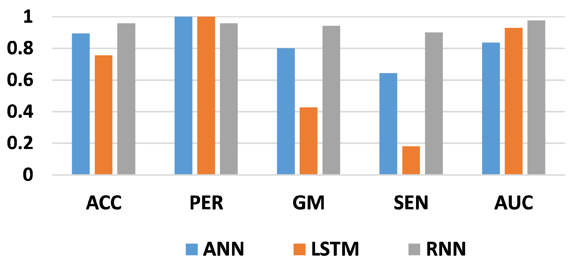
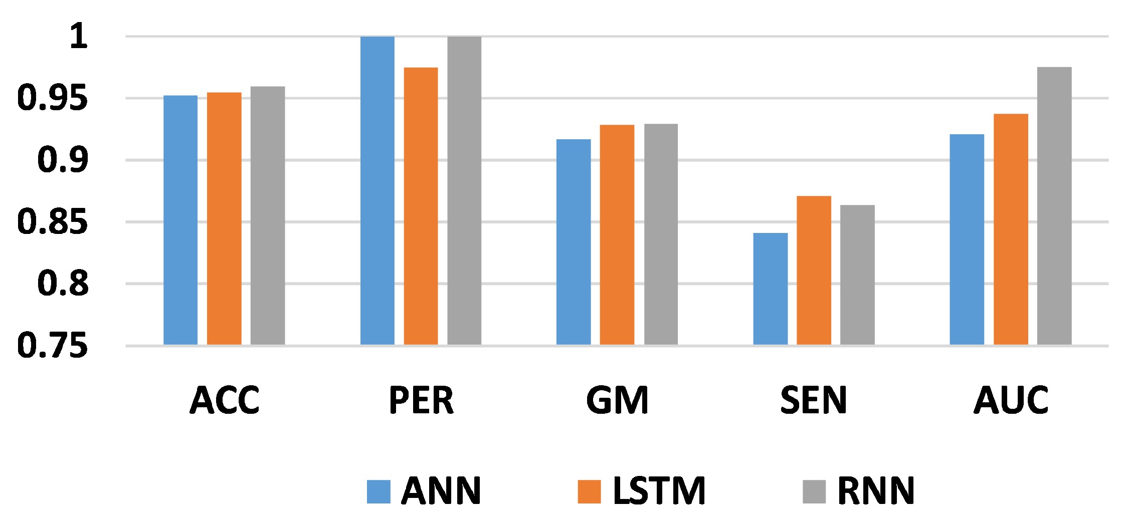
Table 3 shows the obtained results for the three classifiers using the Bayesian algorithm for hyperparameter optimization. The number of iterations is 50. From these results, the best accuracy score, 95.93%, is achieved by the RNN architecture, while the second-best score, 89.93%, is obtained by the ANN model. Moreover, the lowest score, 75.62%, is obtained using the LSTM model. Therefore, the RNN architecture outperforms the other deep learning models in classifying fraud from non-fraud transactions in the credit card dataset. Similarly, the best precision score is obtained with ANN and LSTM, at 1. As a consequence, the two models classify all fraudulent transactions correctly. In contrast, the RNN achieved a score of 95.96% for correctly classified fraud transactions. Taking the G-mean score into account, crucial when two classes have similar importance, this measure demonstrates the model’s ability to distinguish between fraudulent and non-fraudulent transactions. The best G-mean score, 94.18%, is obtained with the RNN model, while the lowest score, 42.64%, is obtained with the LSTM model. In terms of sensitivity score, with the RNN, we obtained 90.15%, while (18.18%) was reached with the LSTM model as the lowest score. Finally, 97.67% is the best AUC score obtained from the RNN architecture. As a result, RNN can be good at detecting fraud transactions based on Bayesian optimization for 50 iterations.
The result of 70 iterations is shown in
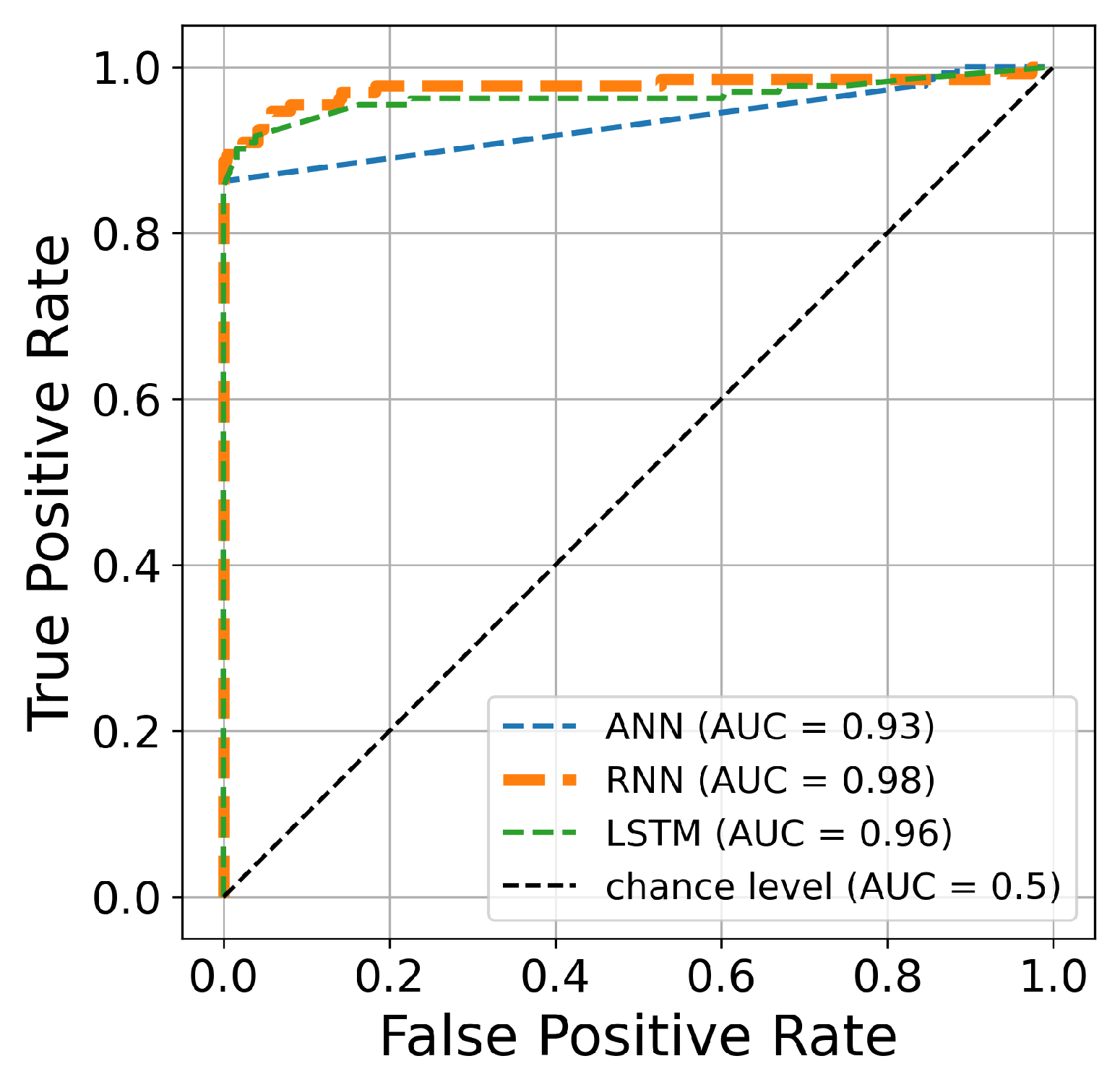
Table 4. It represents the resulting outcome of Bayesian optimization for hyperparameter tuning. These results describe the scores produced by ANN, LSTM, and RNN architectures. The accuracy score for the three classifiers is 95%, indicating that 95% of the transactions are correctly classified. Similarly, we obtained a score of 1 for the precision of LSTM and ANN. The lowest score is achieved by RNN, which correctly classifies 97% of fraud transactions. Furthermore, 92% as the best G-Mean score is achieved by LSTM and RNN. Similarly, we obtained the best sensitivity (87.12%) using the LSTM model and the best AUC using the RNN architecture (97.52%).
Table 5 presents the results obtained for the three models with hyperparameter optimization based on Bayesian optimization for 100 iterations. From these results, we obtained the same accuracy score for the three classifiers, in which 95% of transactions are correctly identified. Furthermore, the best precision score is achieved for both the LSTM and ANN classifiers. On the contrary, ANN obtained the lowest score, at 98% of fraud transactions correctly classified. In terms of G-Mean, we obtained the same score for the three classifiers (92%). Likewise, the same sensitivity is achieved by the three classifiers (86%). Furthermore, the best AUC score was from RNN (97%).
Table 6 shows the computational time for the hyperparameter process. From this table, we notice that the best computational time is that of the ANN architecture, followed by the RNN architecture as the second-best time for hyperparameter searching. So, ANN is faster than RNN, which is faster than LSTM. However, the findings presented in the results table shed light on the impact of hyperparameter optimization iterations on the performance of the three distinct models, ANN, LSTM, and RNN, within the context of our research. Notably, the results showcase varying patterns of performance improvement across different models and iteration counts. For instance, the ANN model demonstrates steady performance gains with each increase in the number of iterations, suggesting a positive correlation between iteration count and model performance. Conversely, the LSTM model exhibits substantial performance improvements as the number of iterations increases, albeit with a slight decline in performance observed at 100 iterations. This possibly indicates the onset of diminishing returns or overfitting. Meanwhile, the RNN model displays notable performance enhancements up to 70 iterations, beyond which further iterations do not yield significant gains, suggesting a potential saturation point in performance improvement. These nuanced insights underscore the importance of carefully optimizing hyperparameters to maximize model performance, while also highlighting the need for monitoring performance trends to avoid potential pitfalls such as overfitting. Overall, these results contribute valuable insights to the field of machine learning and underscore the importance of iterative optimization processes in model development and deployment.
Figure 8,
Figure 9 and
Figure 10 support the results discussed in
Table 3,
Table 4 and
Table 5. The hyperparameter process using RNN is the best choice for detecting fraud in transactions. This approach is more efficient than LSTM and ANN.
As
Figure 11 shows, the hyperparameter optimization process of our system configuration requires a substantial amount of time due to the iterative nature of the loop. Typically, the time required for hyperparameter optimization can vary depending on factors such as the complexity of the dataset and the number of hyperparameters being tuned. In our experiments, this optimization process may take several hours to complete, as it involves iteratively evaluating the performance of different hyperparameter configurations. As for the frequency of optimization, it is crucial to note that this process is not a one-time task. Instead, it may need to be executed whenever there is a significant change in the input dataset or when the performance metrics, such as accuracy, begin to degrade. By periodically re-optimizing the hyperparameters, we ensure that our model remains well-tuned and adaptive to changes in the data distribution or underlying patterns.
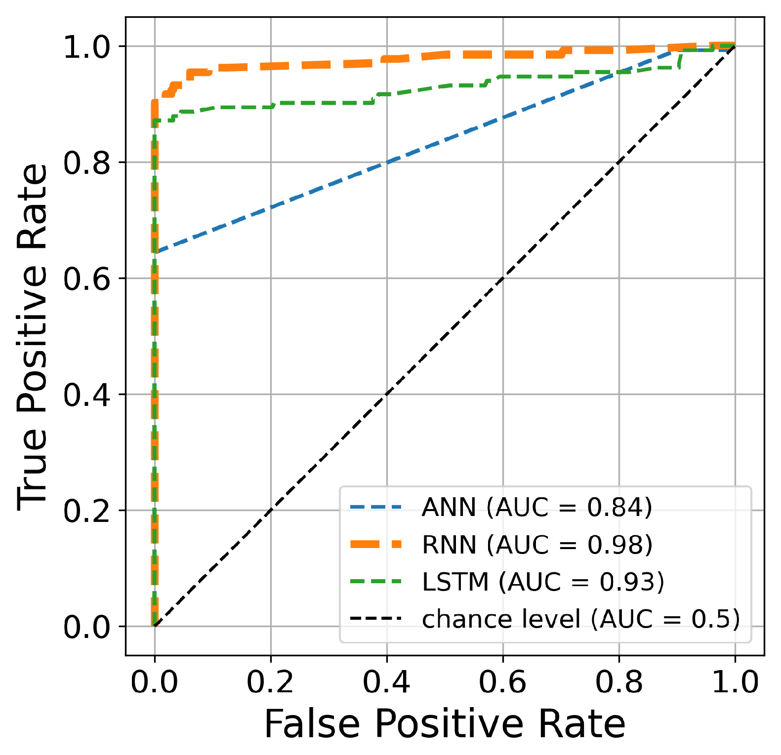
The AUC curve is an efficient and significant estimation of overall performance. It is a general measure of the accuracy of fraudulent transactions. Moreover, a higher AUC curve indicates better prediction performance.
Figure 12,
Figure 13 and
Figure 14 present the AUC curves of the Bayesian algorithm based on hyperparameter optimization for 50, 70, and 100 iterations, respectively, and the three deep learning architectures. The figures confirm the results presented in
Table 3,
Table 4 and
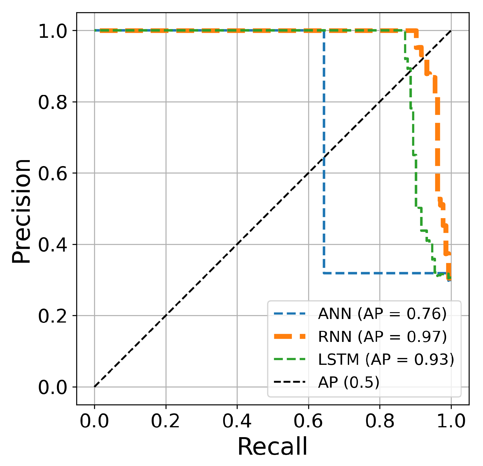
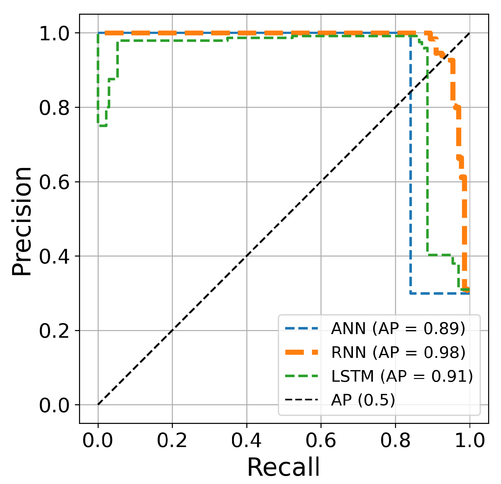
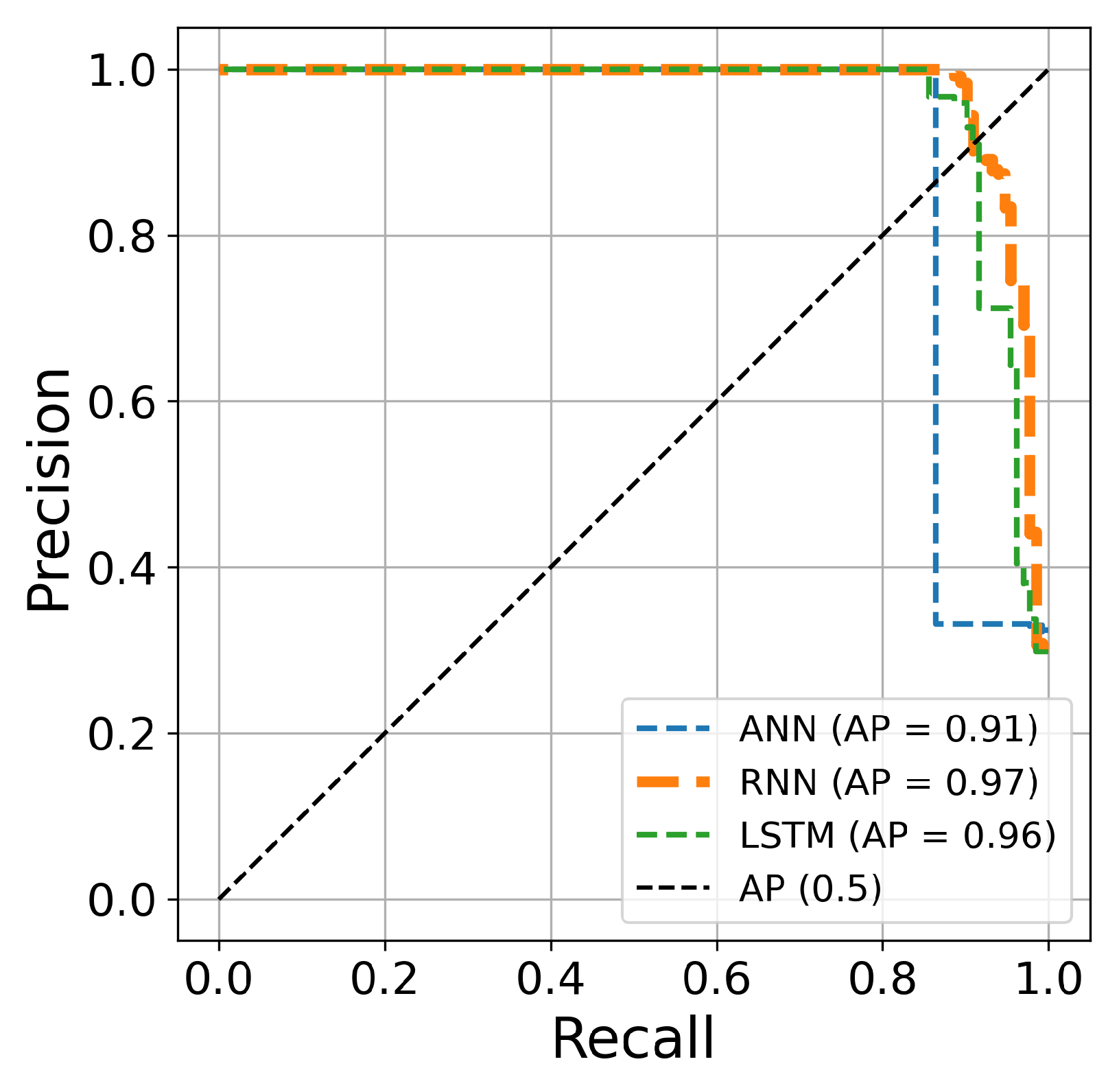
Table 5. The AUC curve of the RNN architecture (orange line) is located closest to the figure’s top-left corner, suggesting that this architecture’s hyperparameter optimization is superior to ANN and LSTM techniques for credit card fraud identification. Another comparison is conducted based on the precision and recall curves. This graph plots the recall score on the x-axis and the precision on the y-axis. The precision–recall curve provides a full picture of the classification performance and is stable even in imbalanced datasets.
Figure 15,
Figure 16 and
Figure 17 clearly show visualizations of the precision–recall plot of the three deep learning architectures based on Bayesian optimization for 50, 70, and 100 iterations, respectively. The precision–recall curve of the RNN approach (orange line) is located closest to the upper right corners of the figures, proving that the RNN architectures for credit card fraud detection achieved better performance for this dataset.
Author Contributions
Conceptualization, S.E.K.; Methodology, S.E.K. and M.T.; Software, M.T.; Validation, S.E.K.; Formal analysis, S.E.K., M.T. and H.S.; Investigation, S.E.K. and H.S.; Resources, M.T.; Data curation, M.T.; Writing—original draft, M.T.; Writing—review and editing, S.E.K., M.T. and H.S.; Visualization, M.T.; Supervision, S.E.K.; Project administration, S.E.K.; Funding acquisition, M.T. All authors have read and agreed to the pubhlished version of the manuscript.
Funding
This research received no external funding.
Institutional Review Board Statement
Not applicable.
Informed Consent Statement
Not applicable.
Data Availability Statement
Acknowledgments
The authors thank the anonymous reviewers for their valuable comments, which have helped us to considerably improve the content, quality, and presentation of this article. The researchers would also like to thank Abderrahim Chalfaouat for reviewing the article’s language.
Conflicts of Interest
The authors declare that they have no known competing financial interests or personal relationships that could have appeared to influence the work reported in this paper.
References
- Abakarim, Y.; Lahby, M.; Attioui, A. An efficient real time model for credit card fraud detection based on deep learning. In Proceedings of the 12th International Conference on Intelligent Systems: Theories and Applications, Rabat, Morocco, 24–25 October 2018; pp. 1–7. [Google Scholar]
- Arora, V.; Leekha, R.S.; Lee, K.; Kataria, A. Facilitating user authorization from imbalanced data logs of credit cards using artificial intelligence. Mob. Inf. Syst. 2020, 2020, 8885269. [Google Scholar] [CrossRef]
- Błaszczyński, J.; de Almeida Filho, A.T.; Matuszyk, A.; Szeląg, M.; Słowiński, R. Auto loan fraud detection using dominance-based rough set approach versus machine learning methods. Expert Syst. Appl. 2021, 163, 113740. [Google Scholar] [CrossRef]
- Branco, B.; Abreu, P.; Gomes, A.S.; Almeida, M.S.; Ascensão, J.T.; Bizarro, P. Interleaved sequence RNNs for fraud detection. In Proceedings of the 26th ACM SIGKDD International Conference on Knowledge Discovery & Data Mining, Virtual, 6–10 July 2020; pp. 3101–3109. [Google Scholar]
- Ahmed, W.; Rasool, A.; Javed, A.R.; Kumar, N.; Gadekallu, T.R.; Jalil, Z.; Kryvinska, N. Security in next generation mobile payment systems: A comprehensive survey. IEEE Access 2021, 9, 115932–115950. [Google Scholar] [CrossRef]
- Dornadula, V.N.; Geetha, S. Credit card fraud detection using machine learning algorithms. Procedia Comput. Sci. 2019, 165, 631–641. [Google Scholar] [CrossRef]
- Tayebi, M.; El Kafhali, S. A weighted average ensemble learning based on the cuckoo search algorithm for fraud transactions detection. In Proceedings of the 2023 14th International Conference on Intelligent Systems: Theories and Applications (SITA), Casablanca, Morocco, 22–23 November 2023; pp. 1–6. [Google Scholar]
- Fang, Y.; Zhang, Y.; Huang, C. Credit Card Fraud Detection Based on Machine Learning. Comput. Mater. Contin. 2019, 61, 185–195. [Google Scholar] [CrossRef]
- Forough, J.; Momtazi, S. Ensemble of deep sequential models for credit card fraud detection. Appl. Soft Comput. 2021, 99, 106883. [Google Scholar] [CrossRef]
- Hu, X.; Chen, H.; Zhang, R. Short paper: Credit card fraud detection using LightGBM with asymmetric error control. In Proceedings of the 2019 Second International Conference on Artificial Intelligence for Industries (AI4I), Laguna Hills, CA, USA, 25–27 September 2019; pp. 91–94. [Google Scholar]
- Kousika, N.; Vishali, G.; Sunandhana, S.; Vijay, M.A. Machine learning based fraud analysis and detection system. J. Phys. Conf. Ser.. 2021, 1916, 012115. [Google Scholar] [CrossRef]
- Tan, G.W.H.; Ooi, K.B.; Chong, S.C.; Hew, T.S. NFC mobile credit card: The next frontier of mobile payment? Telemat. Inform. 2014, 31, 292–307. [Google Scholar] [CrossRef]
- Alarfaj, F.K.; Malik, I.; Khan, H.U.; Almusallam, N.; Ramzan, M.; Ahmed, M. Credit Card Fraud Detection Using State-of-the-Art Machine Learning and Deep Learning Algorithms. IEEE Access 2022, 10, 39700–39715. [Google Scholar] [CrossRef]
- Carcillo, F.; Dal Pozzolo, A.; Le Borgne, Y.A.; Caelen, O.; Mazzer, Y.; Bontempi, G. Scarff: A scalable framework for streaming credit card fraud detection with spark. Inf. Fusion 2018, 41, 182–194. [Google Scholar] [CrossRef]
- Wei, W.; Li, J.; Cao, L.; Ou, Y.; Chen, J. Effective detection of sophisticated online banking fraud on extremely imbalanced data. World Wide Web 2013, 16, 449–475. [Google Scholar] [CrossRef]
- Kim, J.; Kim, H.J.; Kim, H. Fraud detection for job placement using hierarchical clusters-based deep neural networks. Appl. Intell. 2019, 49, 2842–2861. [Google Scholar] [CrossRef]
- El Kafhali, S.; Tayebi, M. XGBoost based solutions for detecting fraudulent credit card transactions. In Proceedings of the 2022 International Conference on Advanced Creative Networks and Intelligent Systems (ICACNIS), Bandung, Indonesia, 23 November 2022; pp. 1–6. [Google Scholar]
- Hajek, P.; Abedin, M.Z.; Sivarajah, U. Fraud detection in mobile payment systems using an XGBoost-based framework. Inf. Syst. Front. 2023, 25, 1985–2003. [Google Scholar] [CrossRef] [PubMed]
- Seera, M.; Lim, C.P.; Kumar, A.; Dhamotharan, L.; Tan, K.H. An intelligent payment card fraud detection system. Ann. Oper. Res. 2024, 334, 445–467. [Google Scholar] [CrossRef]
- Van Belle, R.; Baesens, B.; De Weerdt, J. CATCHM: A novel network-based credit card fraud detection method using node representation learning. Decis. Support Syst. 2023, 164, 113866. [Google Scholar] [CrossRef]
- Jha, S.; Guillen, M.; Westland, J.C. Employing transaction aggregation strategy to detect credit card fraud. Expert Syst. Appl. 2012, 39, 12650–12657. [Google Scholar] [CrossRef]
- Tayebi, M.; El Kafhali, S. Credit Card Fraud Detection Based on Hyperparameters Optimization Using the Differential Evolution. Int. J. Inf. Secur. Priv. (IJISP) 2022, 16, 1–21. [Google Scholar] [CrossRef]
- Mathew, A.; Amudha, P.; Sivakumari, S. Deep learning techniques: An overview. In Proceedings of the International Conference on Advanced Machine Learning Technologies and Applications, Jaipur, India, 13–15 February 2020; Springer: Singapore, 2021; pp. 599–608. [Google Scholar]
- Salloum, S.A.; Alshurideh, M.; Elnagar, A.; Shaalan, K. Machine learning and deep learning techniques for cybersecurity: A review. In Proceedings of the International Conference on Artificial Intelligence and Computer Vision, Cairo, Egypt, 8–9 April 2020; Springer: Cham, Switzerland, 2020; pp. 50–57. [Google Scholar]
- LeCun, Y.; Bengio, Y.; Hinton, G. Deep learning. Nature 2015, 521, 436–444. [Google Scholar] [CrossRef] [PubMed]
- Li, Z.; Pan, Z.; Li, Y.; Yang, X.; Geng, C.; Li, X. Advanced root mean square propagation with the warm-up algorithm for fiber coupling. Opt. Express 2023, 31, 23974–23989. [Google Scholar] [CrossRef]
- Sherstinsky, A. Fundamentals of recurrent neural network (RNN) and long short-term memory (LSTM) network. Phys. D Nonlinear Phenom. 2020, 404, 132306. [Google Scholar] [CrossRef]
- Wang, C.; Niepert, M. State-regularized recurrent neural networks. In Proceedings of the International Conference on Machine Learning. PMLR, Long Beach, CA, USA, 9–15 June 2019; pp. 6596–6606. [Google Scholar]
- Yu, Y.; Si, X.; Hu, C.; Zhang, J. A review of recurrent neural networks: LSTM cells and network architectures. Neural Comput. 2019, 31, 1235–1270. [Google Scholar] [CrossRef] [PubMed]
- Smagulova, K.; James, A.P. A survey on LSTM memristive neural network architectures and applications. Eur. Phys. J. Spec. Top. 2019, 228, 2313–2324. [Google Scholar] [CrossRef]
- Garnett, R. Bayesian Optimization; Cambridge University Press: Cambridge, UK, 2023. [Google Scholar]
- Swinburne, R. Bayes’ Theorem. Rev. Philos. Fr. L’etranger 2004, 194, 250–251. [Google Scholar]
- Dunlop, M.M.; Girolami, M.A.; Stuart, A.M.; Teckentrup, A.L. How deep are deep Gaussian processes? J. Mach. Learn. Res. 2018, 19, 1–46. [Google Scholar]
- Wu, J.; Chen, X.Y.; Zhang, H.; Xiong, L.D.; Lei, H.; Deng, S.H. Hyperparameter optimization for machine learning models based on Bayesian optimization. J. Electron. Sci. Technol. 2019, 17, 26–40. [Google Scholar]
- Credit Card Fraud Dataset. 2023. Available online: https://www.kaggle.com/mlg-ulb/creditcardfraud/data (accessed on 26 December 2023).
- Abdi, H.; Williams, L.J. Principal component analysis. Wiley Interdiscip. Rev. Comput. Stat. 2010, 2, 433–459. [Google Scholar] [CrossRef]
- El Kafhali, S.; Tayebi, M. Generative adversarial neural networks based oversampling technique for imbalanced credit card dataset. In Proceedings of the 2022 6th SLAAI International Conference on Artificial Intelligence (SLAAI-ICAI), Colombo, Sri Lanka, 1–2 December 2022; pp. 1–5. [Google Scholar]
- Hordri, N.F.; Yuhaniz, S.S.; Azmi, N.F.M.; Shamsuddin, S.M. Handling class imbalance in credit card fraud using resampling methods. Int. J. Adv. Comput. Sci. Appl. 2018, 9, 390–396. [Google Scholar] [CrossRef]
- Feurer, M.; Hutter, F. Hyperparameter optimization. In Automated Machine Learning: Methods, Systems, Challenges; Springer: Cham, Switzerland, 2019; pp. 3–33. [Google Scholar]
- Tayebi, M.; El Kafhali, S. Hyperparameter optimization using genetic algorithms to detect frauds transactions. In Proceedings of the International Conference on Artificial Intelligence and Computer Vision, Settat, Morocco, 28–30 June 2021; Springer: Cham, Switzerland, 2021; pp. 288–297. [Google Scholar]
- Tayebi, M.; El Kafhali, S. Performance analysis of metaheuristics based hyperparameters optimization for fraud transactions detection. Evol. Intell. 2024, 17, 921–939. [Google Scholar] [CrossRef]
Figure 1.
Card payment authorization process.
Figure 2.
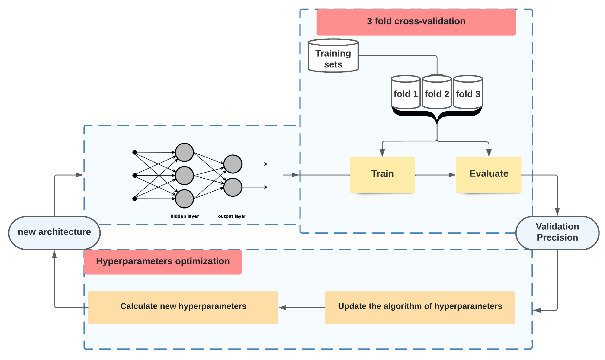
Workflow of deep learning architectures.
Figure 3.
Recurrent neural network architectures.
Figure 4.
Long short-term memory architecture.
Figure 5.
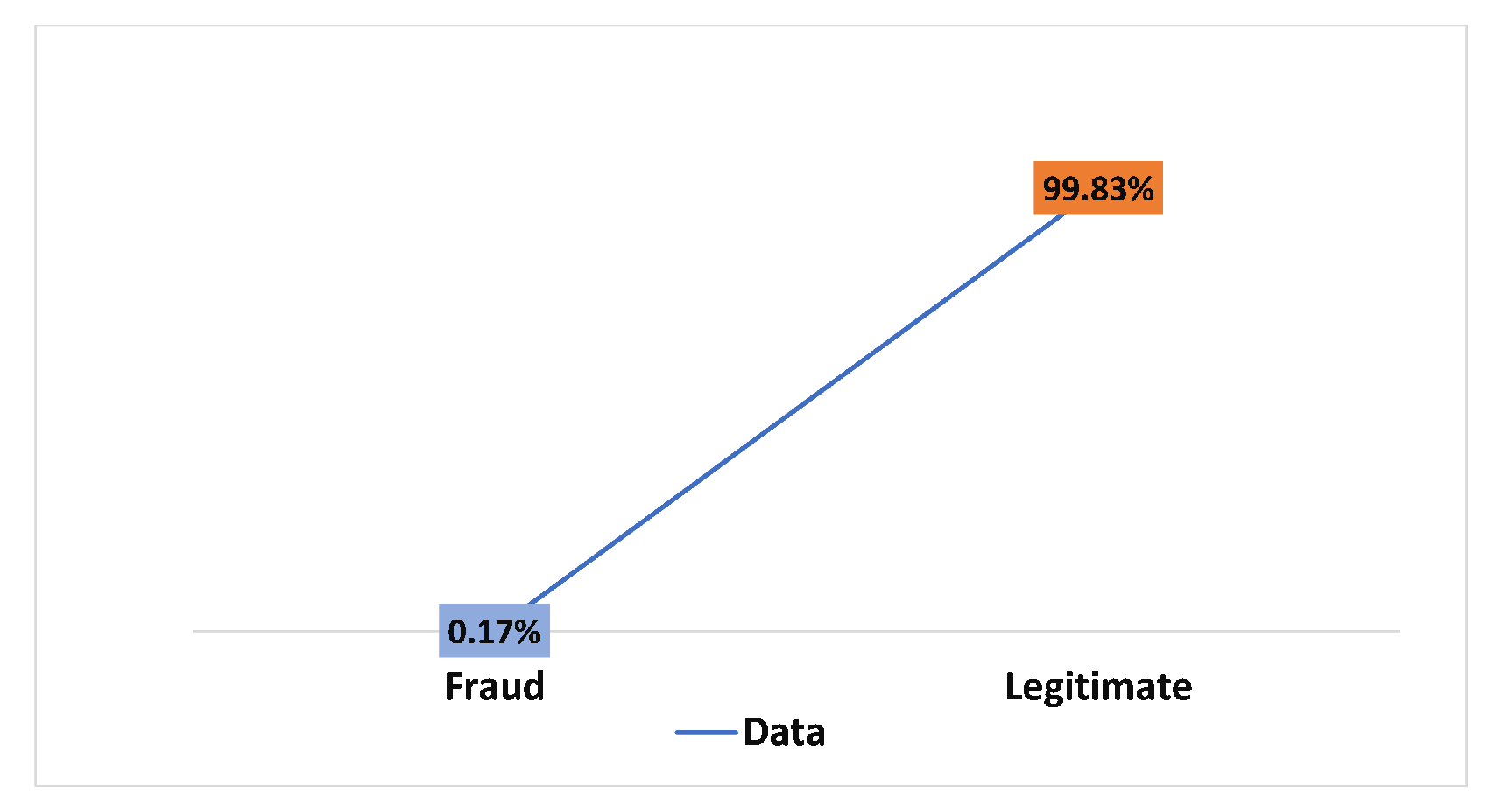
Target variable distribution per fraud and non-fraud transactions.
Figure 6.
Hyperparameter optimization process workflow.
Figure 7.
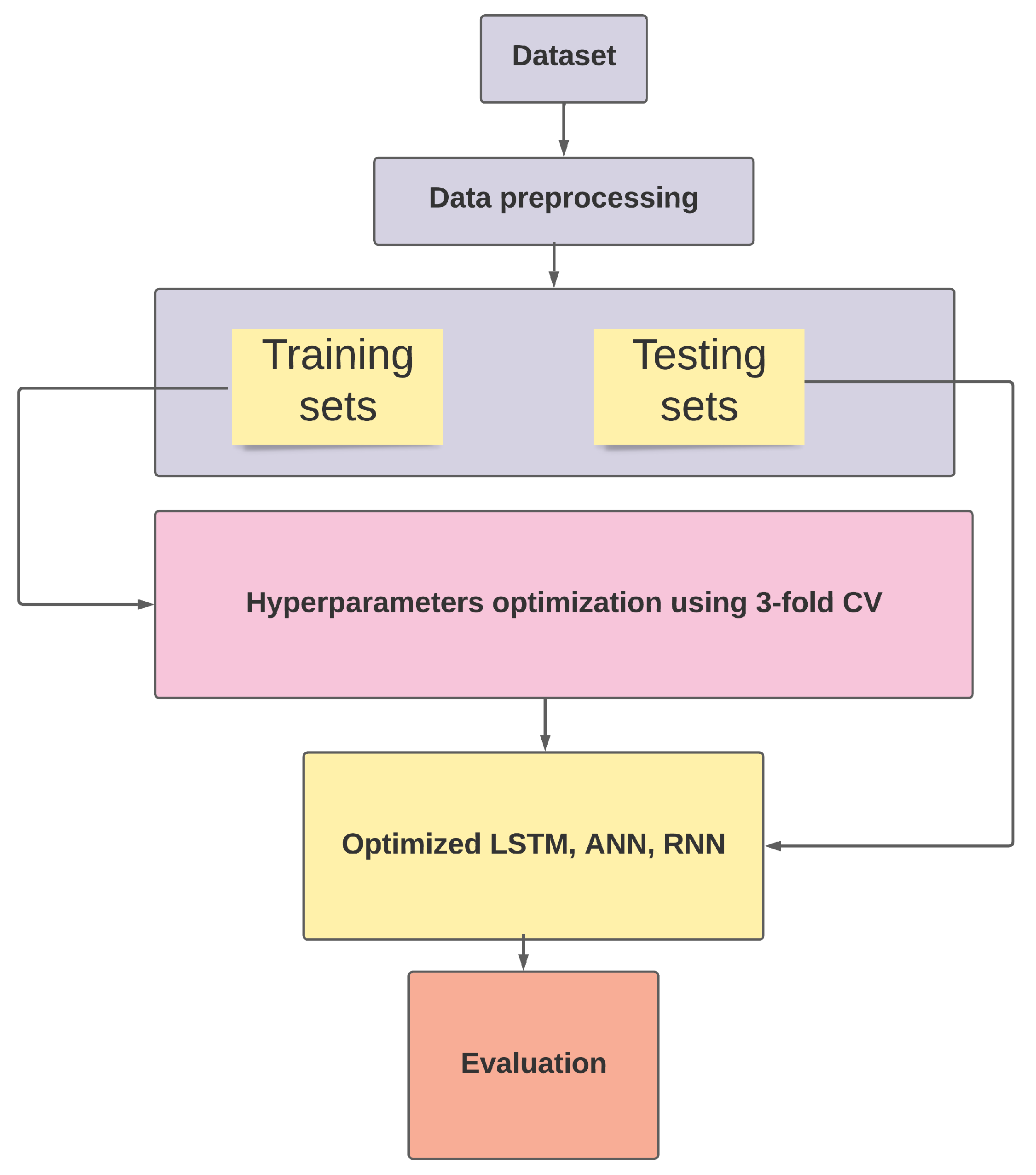
Proposed solution.
Figure 8.
Results of 50 iterations of optimizing the hyperparameters for three deep learning architectures.
Figure 9.
Results of 70 iterations of optimizing the hyperparameters for three deep learning architectures.
Figure 10.
Results of 100 iterations of optimizing the hyperparameters for three deep learning architectures.
Figure 11.
Results of the comparison of hyperparameter optimization execution times.
Figure 12.
The ROC curve constructed after 50 iterations of optimizing hyperparameters using Bayesian algorithm.
Figure 13.
The ROC curve constructed after 70 iterations of optimizing hyperparameters using Bayesian algorithm.
Figure 14.
The ROC curve constructed after 100 iterations of optimizing hyperparameters using Bayesian algorithm.
Figure 15.
The precision–recall curve constructed after 50 iterations of optimizing hyperparameters using Bayesian algorithm.
Figure 16.
The precision–recall curve constructed after 70 iterations of optimizing hyperparameters using Bayesian algorithm.
Figure 17.
The precision–recall curve constructed after 100 iterations of optimizing hyperparameters using Bayesian algorithm.
Table 1.
Features description.
| Variable | Definition | Type |
|---|
| Class | Target feature in this dataset. Takes two values: 0: Legitimate; 1: Fraud | Categorical |
| Amount | The amount of the transaction sample | Numeric |
| Time | The difference in time between the first and the current transactions, in seconds | Numeric |
| V1 to V28 | Features transformed using PCA technique to protect cardholders’ privacy and confidentiality | Numeric |
Table 2.
Search space for hyperparameter optimization.
| Hyperparameter | Optimization Rate | Type |
|---|
| Activation function | | Categorical |
| Learning rate | | Continue |
| Dropout rate of layer 1 | | Continue |
| Dropout rate of layer 2 | | Continue |
| Batch size | | discrete |
| Epochs | | discrete |
| Number of neurons in layer 1 | | discrete |
| Number of neurons in layer 2 | | discrete |
| Number of LSTM Units in layer 1 | | discrete |
| Number of LSTM Units in layer 2 | | discrete |
| Number of RNN Units in layer 1 | | discrete |
| Number of RNN Units in layer 2 | | discrete |
Table 3.
Results obtained using the Bayesian algorithm for 50 iterations.
| Model | ACC | PER | GM | SEN | AUC |
|---|
| ANN | 0.8939 | 1 | 0.8024 | 0.6439 | 0.8356 |
| LSTM | 0.7562 | 1 | 0.4264 | 0.1818 | 0.9291 |
| RNN | 0.9593 | 0.9596 | 0.9418 | 0.9015 | 0.9767 |
Table 4.
Results obtained using the Bayesian algorithm for 70 iterations.
| Model | ACC | PER | GM | SEN | AUC |
|---|
| ANN | 0.9525 | 1 | 0.9170 | 0.8409 | 0.9207 |
| LSTM | 0.9548 | 0.9745 | 0.9288 | 0.8712 | 0.9372 |
| RNN | 0.9593 | 1 | 0.9293 | 0.8636 | 0.9752 |
Table 5.
Results obtained using the Bayesian algorithm for 100 iterations.
| Model | ACC | PER | GM | SEN | AUC |
|---|
| ANN | 0.9548 | 0.9827 | 0.9263 | 0.8636 | 0.9323 |
| LSTM | 0.9571 | 1 | 0.9252 | 0.8560 | 0.9641 |
| RNN | 0.9593 | 1 | 0.9293 | 0.8636 | 0.9752 |
Table 6.
Execution time results for hyperparameter optimization for different iterations.
| Model | 50 Iterations | 70 Iterations | 100 Iterations |
|---|
| ANN | 604.66 | 737.03 | 1045.28 |
| LSTM | 1395.57 | 2761.79 | 2603.52 |
| RNN | 1039.28 | 1934.66 | 1934.66 |
| Disclaimer/Publisher’s Note: The statements, opinions and data contained in all publications are solely those of the individual author(s) and contributor(s) and not of MDPI and/or the editor(s). MDPI and/or the editor(s) disclaim responsibility for any injury to people or property resulting from any ideas, methods, instructions or products referred to in the content. |
© 2024 by the authors. Licensee MDPI, Basel, Switzerland. This article is an open access article distributed under the terms and conditions of the Creative Commons Attribution (CC BY) license (https://creativecommons.org/licenses/by/4.0/).


