1. Introduction
We developed a generally applicable Q-compression method for solving specific mixed-integer graph optimization problems. Our approach is based on a dynamic discrete representation of the mixed-integer state space and provides a human-interpretable solution to the curse of dimensionality issue. The efficiency of our method is demonstrated on selected use cases that belong to a common problem class of constrained stochastic graph traversal problems.
We identified a diverse set of problems that belong to the class of constrained graph traversal problems. Although the shortest pathfinding problem is a well-known combinatorial optimization problem, its parameters are difficult to define exactly [
1]. It is easy to see that the optimal route problem of a truck is practically a constrained shortest pathfinding problem [
2], where the constraints describe the working hours limits of the driver and the availability of parking or the fuel capacity limits [
3]. Daily planning of the route of an electric delivery van is a constrained Hamiltonian pathfinding problem, where the constraints are based on the limits of battery capacity [
4] and charging options [
5] or battery exchange opportunities [
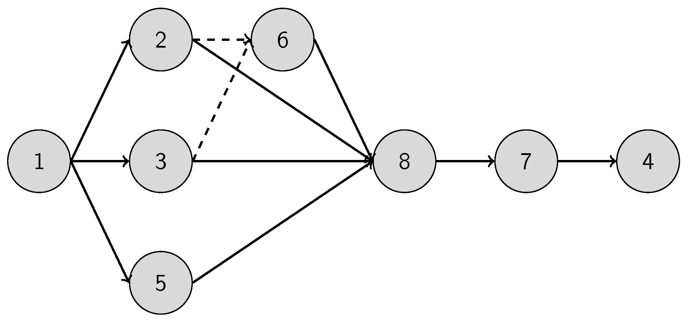
6]. Furthermore, disassembling all components of a product after its life cycle is also a constrained graph traversal problem, where a precedence graph describes component removal dependencies, and the constraints limit the use of parallel workstations [
7]. Finally, we would like to highlight that in real-life problems, these kinds of problems are rather stochastic optimization tasks than discrete [
8,
9].
The constrained shortest pathfinding problem (CSPP) is shown to be NP-complete, and furthermore, the Hamiltonian pathfinding problem can be transformed into an SPP in polynomial time [
10]. It is also presented that disassembly optimization problems can be solved by formulating as an SPP [
11]. It is easy to see that these problems originate from one common root, which is based on CSPP. Therefore, a solution for other types of problems within the problem class can be derived from a CSPP solution.
Traditional methods for the shortest pathfinding problem, such as Dijkstra’s [
12], Floyd-Warshall [
13], and Bellman-Ford algorithms, deliver the optimal solution in a reasonable time but are not able to handle stochastic distance distributions and complex constraints. The exact mixed-integer linear or quadratic programming technique [
14] can be an option in multiple cases because it supports the integration of constraints, but is sensitive to stochastic parameters and the size of the problem [
15]. There are successful results in applying machine learning (ML) tools to improve the performance of branch & bound method by optimizing the plane cuts. However, the optimal strategy depends significantly on the nature of the problem, and hence, it is hard to generalize the method [
16]. The genetic algorithm demonstrated its power in stochastic search problems and converges to the Pareto-optimal solution. It provides not only the best solution, but also alternatives, but requires built-in heuristics to retain cycles in the path, and its performance strongly depends on the right parameterization setup [
17]. In summary, there are no general methods to solve constrained stochastic graph traversal problems, so we propose to use the reinforcement learning approach, which can handle both stochastic challenges and constraints well [
18].
Reinforcement learning (RL) can be an obvious solution for sequential decision-making processes such as step-by-step pathfinding [
19]. The objective function should be implemented in the reward function, as well as in violation of constraints [
20]. However, by considering some stochastic effect or measurement uncertainty, additional difficulties arise: some continuous components need to be integrated into the state space, which becomes mixed discrete-continuous.
Mixed-integer programming covers a general framework for a wide range of optimization problems, such as scheduling, routing, production planning, and other graph optimization tasks [
21]. As mixed-integer programs (MIPs) are hard to solve problems, their effective solvers rely on heuristics. Heuristics have variable performance in different types of problems, leading to a heavily human-supervised solution design. As the number of optimization tasks increases exponentially, there is a need for a higher level of autonomous processes for optimal decisions. Reinforcement learning (RL) can serve as a valuable tool in the development of self-optimizing solutions.
There are already several directions for applying RL techniques to solve MIPs. Deep reinforcement learning (DRL) can be used to find a feasible solution to MIPs applying the Smart Feasibility Pump method [
22]. RL can be applied to determine the optimal cutting plane as a subroutine of a modern IP solver [
23]. Gradient-based RL methods can be extended to use mixed-integer model predictive control (MPC) for an optimal policy approximation [
24]. A general integer programming (IP) solver technique was developed to learn the large neighborhood search (LNS) policy for IP [
25], but the method does not handle the stochastic constraints yet. Constrained combinatorial optimization problems can also be solved by RL techniques [
26]. Moreover, stochastic shortest-path problems also have RL solutions [
27]. In contrast with these solutions of mixed-integer optimization problems, we developed a new discretization approach for reducing the state-space into a purely discrete space representation by performing the DBSCAN clustering method and applied an iterative policy optimization method to that.
Our contributions are as follows.
We define the class of constrained stochastic graph traversal problems by identifying several real-life problems that belong to that. Although the pairwise relationships of individual problems were already known, we recognized that their joint investigation is recommended.
We present a general end-to-end process for collecting observations, creating and fine-tuning the discretization function based on DBSCAN clustering results, building a Q-table, and using it for optimal decisions. We call our framework the Q-table compression method.
Our solution delivers a human-interpretable model without a complex pre-study of the correlation of distances or further hidden dependencies.
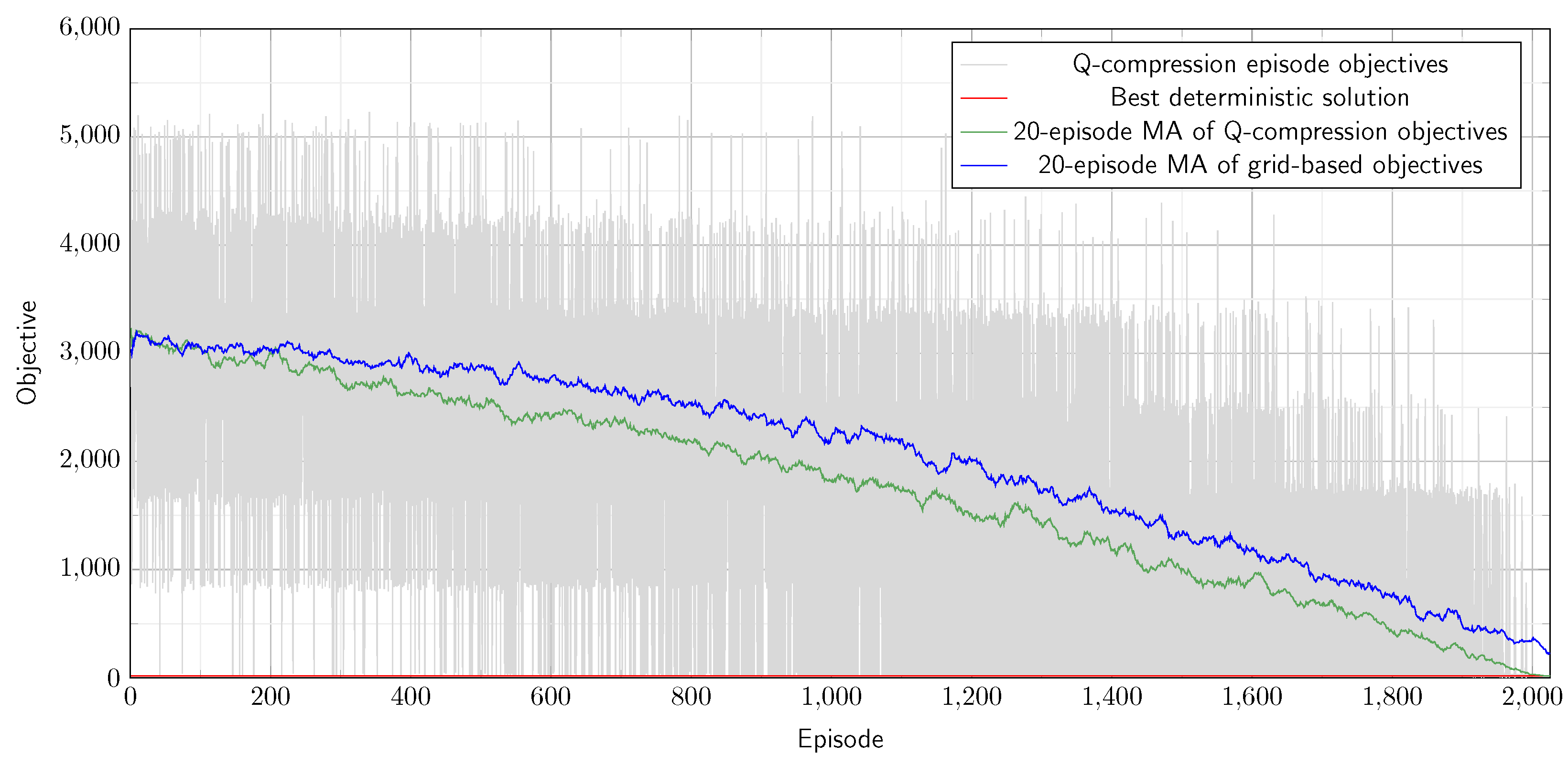
We demonstrate the usability of our method in three selected use cases belonging to the problem class of constrained stochastic graph traversal problem: in a constrained stochastic shortest pathfinding problem, in a constrained stochastic Hamiltonian pathfinding problem, and in a stochastic disassembly line balancing problem. We also verify the performance of the Q compression method compared to a simple grid-based discretization method.
In
Section 2, we define the class of constrained stochastic graph traversal problems and formulate the constrained shortest pathfinding problem (CSPP), the constrained Hamiltonian pathfinding problem (CHPP), and the disassembly line balancing problem (DLBP). We also show that a solution for CSPP can be used directly for CHPP and DLBP as well. In
Section 3, we will present a new multistep method, called the Q-table compression method, which integrates different state-space reduction steps with a dynamic training sampling technique to deliver an adaptive policy iteration algorithm. In
Section 4, we demonstrate the applicability of our algorithm to three selected use cases: a CSPP, a CHPP, and a DLBP example. In
Section 5, we give a summary and conclusions, and we will describe some further research directions and open research questions.
2. Constrained Graph Traversal Problem Formulation
Due to the rapid development of technology and economics, optimization problems are increasingly being focussed on to further increase efficiency. There are numerous proven methods for finding optimal solutions for certain tasks, but there are cases where the classical methods cannot be applied directly or do not perform well. We present a special optimization problem class for which no general solution is known. We will formulate the problem and show that multiple real-world problems belong to the class.
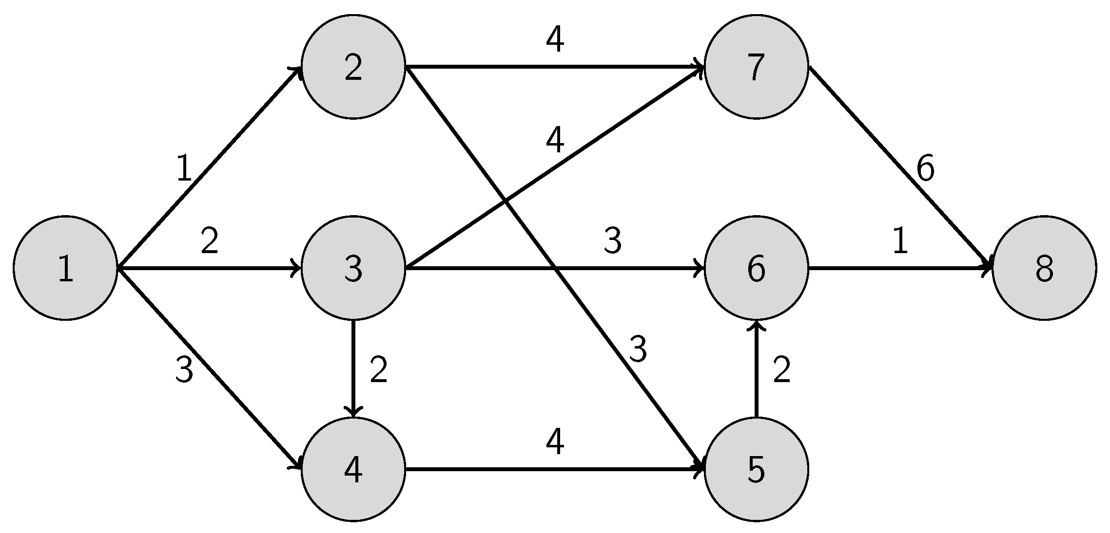
Consider a weighted directed graph . The vertex set is denoted by , while the edge set is described by and finally the corresponding positive distances are in . We can use the function as an assignment to identify the corresponding distance of an edge: for all . The graph is assumed to be connected and simple in the context that there are no self-loops or multi-edges in it. The edge that connects the vertex i and the vertex j can be referred to as .
Suppose that the graph has two privileged vertices: s and t are the starting vertex and the target vertex. A path is defined as a series of edges: . The shortest pathfinding problem (SPP) is to find a path from s to t with the shortest total distance: , where , and is the distance value of the edge .
We can add further limitations on the shortest pathfinding problem: assume that the traveler can cover only a limited distance in one go, hence the shortest path should be split into subroutes or ranges that do not exceed their distance limit L: , where for all . It is easy to see that .
An important relevance of a constrained shortest path problem in practice is the truck routing problem: in this case, the traveler should split his route into feasible ranges due to the driver’s working hours limits and parking availability or fuel capacity limits. A secondary goal is to minimize the number of ranges in the whole path. To reach this, it is mandatory to extend the objective of the classical shortest pathfinding problem, and declare the common scale for it, which can be the cost:
where
represents the distance proportional cost of the completed path and
covers the range cost (e.g., battery recharge cost). We refer to this problem type as the constrained shortest pathfinding problem (CSPP).
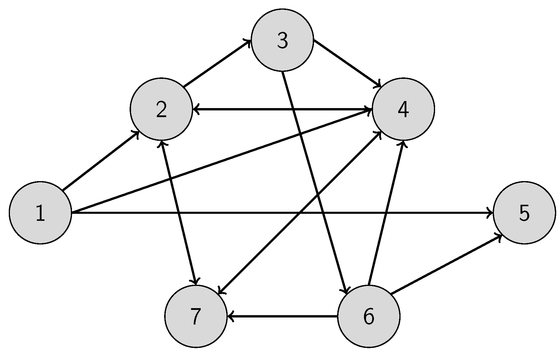
There are other problems that can be transformed into a CSPP. Consider a directed connected graph . The Hamiltonian pathfinding problem is to find a continuous path in the graph that visits all the vertices exactly once. The problem can be reduced to a shortest pathfinding problem. We can perform a reversible transformation on graph to prepare graph as follows:
Every possible loop-free route declares a vertex in the transformed graph, including which represents the empty subset.
is an edge in the transformed graph if and only if:
- -
The path in
represented by
is a sub-path of the one represented by
:
- -
The path of
is longer exactly by one edge than the path of
:
- -
By marking with
the last element of
, the additional edge of path
is at its end compared to the path of
:
- -
The initial vertex can be freely chosen from all vertex
As in the classical Hamiltonian pathfinding problem in our formulation, there were no distances in the original graph , but the SPP formulation requires distances to the edges, so we can assign a constant value 1 to all existing edges of the transformed graph . However, in real-world problems, there are given distances: and we are interested in solving the shortest Hamiltonian pathfinding problem (SHPP).
Finally, an optimal solution to the shortest path finding problem of will provide the shortest Hamiltonian path with an objective function of .
We can simplify the graph by merging vertex pairs and into a single transformed vertex if both contain the same original vertices and their last elements are identical. (For example, can be merged into , but cannot be merged into ). The merging concept comes from the observation that it does not matter in a route what the vertex visiting order was, only the fact whether a vertex was visited or not and the last visited vertex, which determines where the traveler can move on. Denote by those transformed vertices that contain all . Then it can be shown that finding a Hamiltonian route in graph indicates a path from to in , and vice versa.
Similarly to CSPP, a further constraint can be introduced to limit the distance that the traveler can cover in one go. Formally, the Hamiltonian path should be split into subroutes or ranges that do not exceed their distance limit L: , where for all . It is easy to see that .
The objective of the constrained shortest Hamiltonian pathfinding problem (CSHPP) will contain a second term to minimize the number of required ranges:
where
represents the proportional cost of the distance of the completed path and
covers the range cost.
A relevant practical problem type is the daily route planning of an electric delivery van where all the target addresses should be visited by taking into account the limits of the battery capacity and the charging options or the battery exchange opportunities.
Another type of problem that can be transformed into a CSPP is the disassembly line balancing problem. In its simplest form, we consider a disassembly line for a single product with a finite supply. Each product has
n elementary components to remove, represented by a vertex set
. The task of eliminating the component
is specified by its processing time
, while a boolean flag of
indicates its hazardousness, and finally
declares the demand value of it. The general problem is to determine the disassembly order of the components and assign every task to the workstations of the disassembly line to optimize the objective function. The pre-defined cycle time is denoted by
, and each workstation should complete its assigned removal tasks within the cycle time. A directed precedence graph
describes the logical dependencies of component removal tasks. As we mentioned above, the vertices represent the components to be removed. The removal process of a component
can be started only if all components from which a directed edge goes to the vertex
are already removed. Typically, the precedence graph is used in its transitive reduced form. Consider a feasible solution that declares the order of component removals: the component represented by the vertex
should be removed as the
th element, and
determines which component should be removed on the workstation
i as the
jth task. Then the objective function can be formulated as follows:
The first term determines the quadratic idle times of the used workstations, which supports not only minimizing idle times but also decreasing imbalance. The second and third terms depend on the component property and disassembly sequence and aim to remove the hazardous components and the components with higher values earlier. The three terms are weighted by
,
, and
, which have multiple goals behind them: compensating for the scaling discrepancies of the objectives and determining the relative importance of the objective components based on external preferences.
It is easy to see that the disassembly line balancing problem is a special modified case of a constrained Hamiltonian pathfinding problem since all the components should be removed. However, on the one hand, the disassembly of the components depends not only on the last removed components but also on the previously removed components, and on the other hand, the objective function is more complex, with a quadratic term in it. Similarly to the Hamiltonian pathfinding problem, we can construct a reversible transformation
to formulate a problem as a CSPP to produce graph
, for which the objective function becomes to the following form:
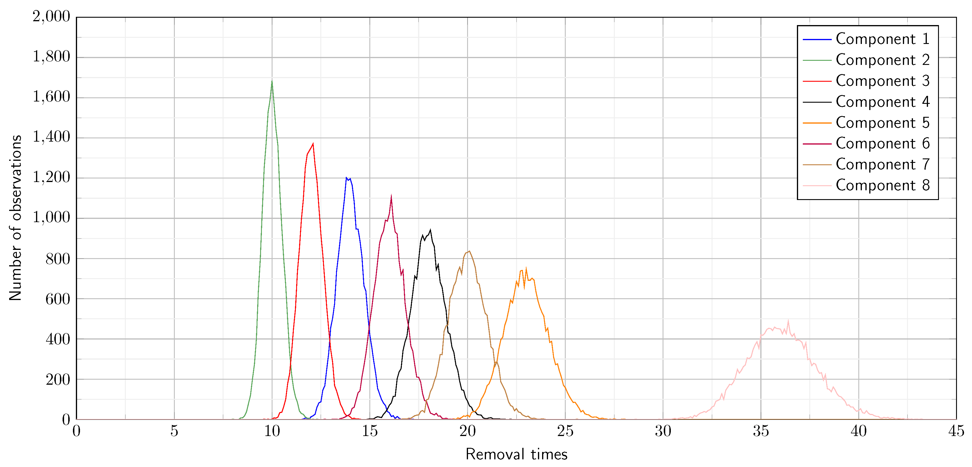
In the real world, the previously described problems are rather stochastic than deterministic: in the routing problems, the distances are measured on a time scale that depends on the traffic, the weather, and further external conditions, while in the disassembly problems, the component removal times depend on the product conditions.
In the formulation of stochastic shortest pathfinding problems, the directed graph has the same structure as in the deterministic case, so the vertex set and the edge set are identical, but the related distances are probability variables: .
Classical solution methods are not directly applicable to the types of problems formulated above, or their resource requirements increase radically for larger problems. This led us to turn to the reinforcement learning method which demonstrated its ability to approach the optimal solution efficiently.
3. Q-Table Compression Method
In this section, we present a discretization method integrated into the Q-table-based policy iteration algorithm to solve mixed continuous-discrete problems with a reinforcement learning approach. First, we summarize the key properties of reinforcement learning by highlighting the action-value-based policy iteration methods, especially the every-visit Monte Carlo method and the Q-learning concept. Then we declare the basic requirements for a state compression solution. Finally, we describe the Q-table compression process in detail by providing the pseudo-algorithm to support its implementation.
3.1. Reinforcement Learning (RL)
Reinforcement learning (RL) solves problems due to sequential learning. An agent takes observations () of the environment and, based on that, executes an action (). As a result of the action in the environment, the agent will receive a reward (), and it can take a new observation () from the environment, and the cycle is repeated. The problem is to let the agent learn to maximize the total expected reward.
Preliminary, we should highlight that graph traversal problems can be approached as a sequential decision problem: the agent observes the traveled path, which is a sequence of the visited vertices, and needs to decide on the next action that should define the next vertex to visit. Therefore, RL techniques can provide an obvious solution for graph traversal problems by determining a sequence of vertices to find an optimal (shortest) path.
Reinforcement learning is based on the reward hypothesis, which states that maximization of expected cumulative rewards can describe all goals. Formally, the history is the sequence of observations, actions, and rewards: . The state is the information used to determine what happens next. Formally, the state is a function of the history: . A state is Markov if and only if . Markov property is fundamental to the theoretical basis of RL methods. denotes the total discounted reward of the time step t: . According to these, for a graph traversal problem, the action space is practically the vertex set: , the observation space is the subroute performed: , while the reward is the increment of the partial objectives:
The state value function gives the expected total discounted return if starting from state s: . The Bellman equation practically states that the state value function can be decomposed into two parts: immediate reward () and the discounted value of successor states .
The policy covers the agent’s behavior in all possible cases, so it is essentially a map from states to actions. There are two main categories in it: deterministic policy () and stochastic policy ().
We will focus on using an action-value function to determine the current optimal action. However, it can be a very slow process for large state- and/or action spaces to keep the value function updated (and hence optimal). Denote by the counter of visiting the state s with an action selection of a. Then consider the function , which accumulates the expected total discounted reward starting from state s and choosing action a. According to the every-visit Monte Carlo policy evaluation process, if the agent performs a new episode and receives rewards accordingly, then the counter must be incremented: , and the Q-value function must be updated for all visited pairs: . It is proven that if the agent follows the update of the Q value function combined with a simple -Greedy action selection method, then the Q-value function approaches the optimal policy as the number of observations tends to infinity.
There are several situations where the learning process is not based only on the agent’s own experience. Formally, this means that action-value function is determined by observing the results of an external behavior policy .
A possible way to handle the difference between the target and behavior policies is to modify the update logic of the value function as Q-learning does (Section 6.5 in [
28]). Assume that in state
the very next action is derived by using the behavior policy:
. By taking action
immediate reward
and the next state
will be determined. But for the update of the value-function, let us consider an alternative successor action based on target policy:
. Then the Q-learning value-function update will look like:
.
In a special case, if the target policy is chosen as a pure greedy policy and the behavior policy follows -greedy policy, then the so-called SARSAMAX update can be defined as follows: . Last, but not least, it was proven that Q-learning control converges to the optimal action-value function: .
In our solution, we used the every-visit Monte Carlo method to determine the optimal policy. However, this can be easily replaced by Q compression, but in that case, it is necessary to choose a suitable -strategy.
3.2. Q-Table Compression Process
In this section, we collect the basic requirements of a discretization function, then present the Q-table compression process in detail, and highlight some hints and guidelines for implementation.
In general, Q-table methods are used for discrete problems. However, there are cases where the discrete problems partially become continuous by considering some stochastic effect or measurement uncertainty. One option to decrease the complexity of such a problem is to divide it into sub-problems. It can be done by introducing sub-goals and solving these problems separately [
29]. Another option is to merge those observed states into a common one that differs from each other only insignificantly. This can be done by introducing a grid representation over the continuous observation space [
30]. In this section, we will present an integrated method to dynamically redefine the state space and transform the Q-table to align it to the changes. We assume a stochastic Markov Decision Process with a mixed-integer state space and discrete action space.
denotes the jth observation in episode i, and it is an element of the observation space O. Our goal is to define a discrete representation S that will be used as a state space in the reinforcement learning process. Formally, we are looking for an iteratively refined mapping function .
We can declare the following requirements for the functions .
Let’s assume that the optimal action is determined for each and every and it is denoted by . If then . This practically means that the mapping function merges observation states only if their optimal actions do not differ.
The mapping function should be consistent in that sense that if action moves the agent from the observation state to then action should move the agent from to .
, or in other words: the size of the state representation S should be significantly smaller than the size of observation space O. The smaller S is the better representation.
The first requirement prevents merging states that have different optimal actions. The second defines the transitivity of the mapping function. The last requirement states that the potential of using the described representation function depends on the efficiency of dimension reduction: if no significant reduction can be reached, then the method cannot raise the efficiency of the learning process.
According to the above requirements, we design a modified Q-table-based policy iteration method by integrating a discretization step into it. In the simplest RL framework, the agent observes its states directly and takes its actions accordingly. In our approach, the agent takes observations, determines the simplified state, and takes actions based on it. So observations determine the state, but observation space differs from state space: the first one is a mixed-integer space, while the last one is purely discrete. The key component in the process is the state space definition and its projection.
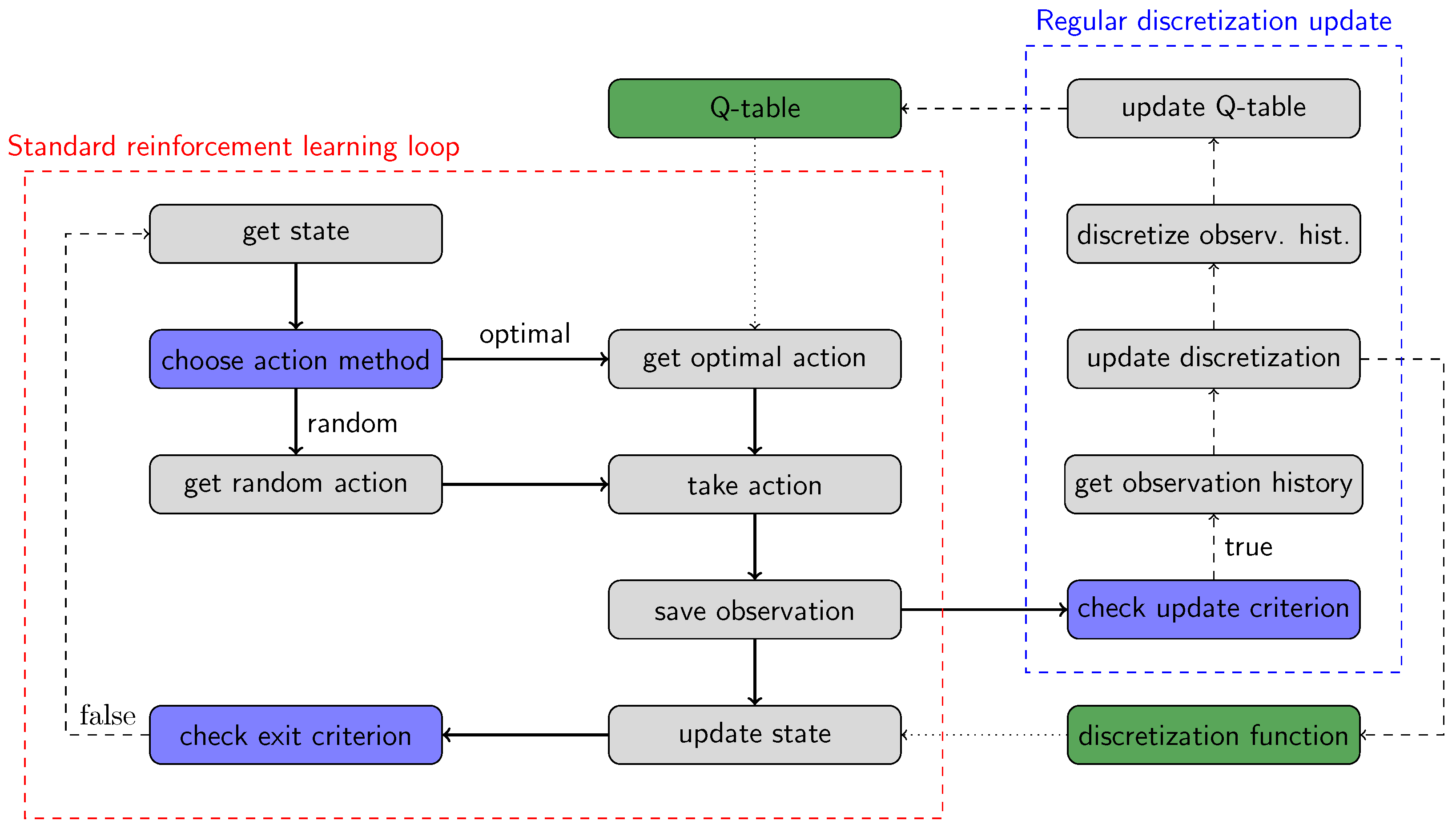
We suggest maintaining a compression-based Q-table learning process due to the following steps, which are summarized in
Figure 1.
There is a standard reinforcement learning loop in the process. The agent queries its current discretized state (get state). The learning process is based on the -Greedy algorithm: the agent decides whether to take a random action or take the best-known action (choose action method). The agent randomly chooses an action with probability of the feasible actions (get random action), or chooses the optimal action from the feasible actions with probability (get optimal action). In this case, the agent determines the expected cumulative rewards to reach the target state for all feasible actions first and then chooses the action with the best total expected reward (or if there are multiple actions with the same total expected reward, then randomly choose one out of them). If the Q-table does not contain a relevant entry for the current state because the trajectory is undiscovered, then the action selection falls back to the random method. The value of the parameter decreases from 1 to 0 linearly as the number of episodes goes to its predefined limit. We would like to highlight that the restriction on potential actions improves the efficiency of the learning process compared to enabling any action and producing a bad reward for unfeasible actions.
Once the action is chosen, the agent performs the selected action, determines the new observation state, and registers the reward (take action). After that, the agent saves the quadlet (old state, action, new state, reward) into the observation history (save observation), and determines the new discretized state by applying the discretization function for the observation (update state). Finally, the agent checks whether the target state has been reached (check exit criterion). If not, then the cycle repeats.
Next to the standard reinforcement learning loop, the agent needs to update the discretization regularly, and on top of that, compress the state space size. The discretization update process is quite resource-intensive. Therefore, we suggest performing it after a batch of episodes. Once, when the update criterion is satisfied (
check update criterion) the agent queries the observation history (
get observation history). To let the agent act adaptively, the history can be accessible due to a moving observation window to get the most relevant part of the history and not process the old, invalid records from there. The major goal at this stage is to create a new/updated discretization ruleset that fits the requirements as described above in this subsection and projects the mixed discrete-continuous observation space to a discrete state space (
update discretization). Denote by
an observation, where
shows the currently visited vertex of the graph, and
describes the current range utilization. The agent takes the observations in a loop: It fixes the discrete part of the observation space (practically a vertex) and queries all matching records:
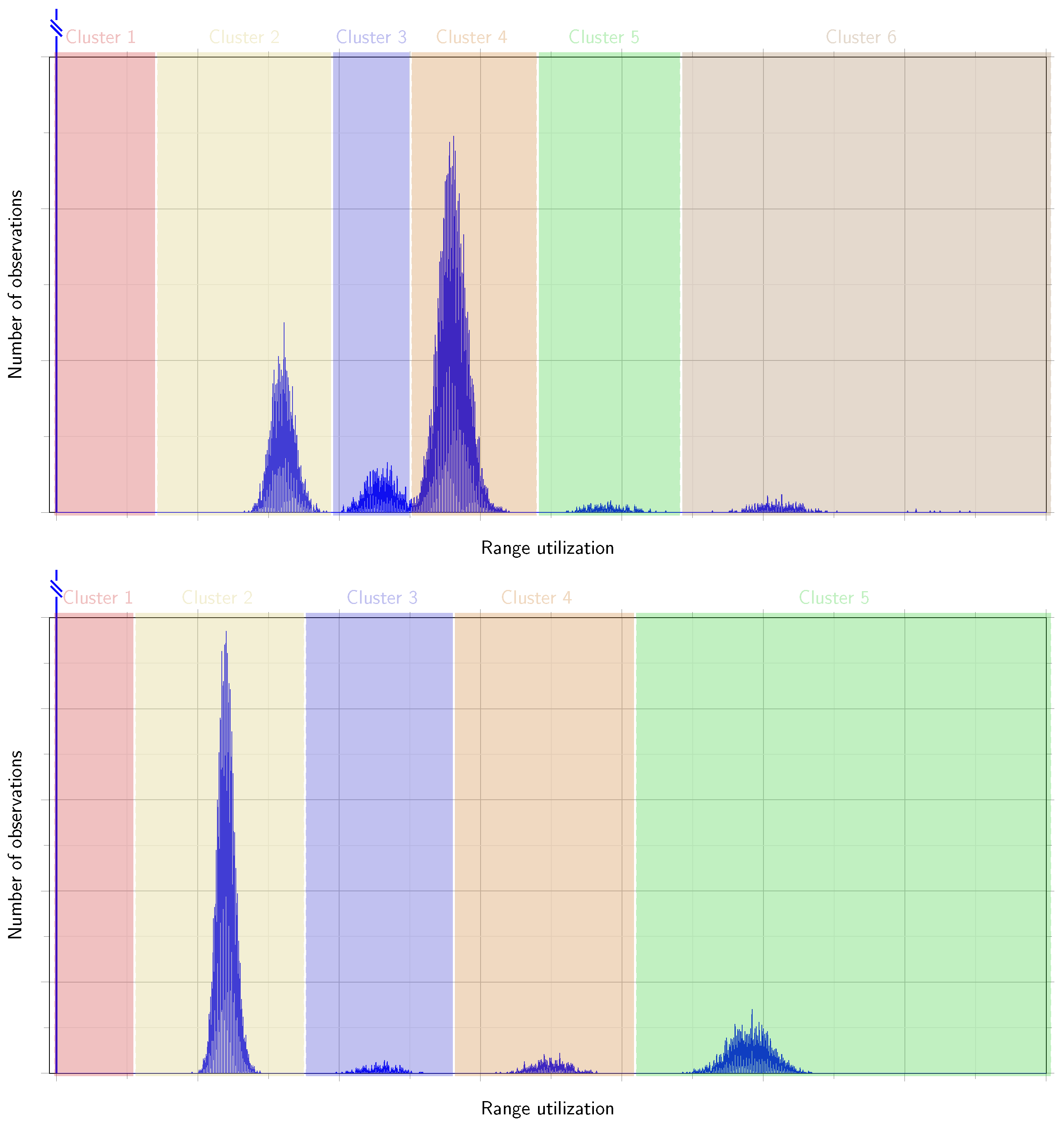
. Then it uses the DBSCAN algorithm to assign the continuous range utilization values of the observations into clusters. Denote
the
ith range of the corresponding cluster and
the number of identified clusters of the vertex
v. The ranges should be nonoverlapping:
for all
, and they need to be widened to completely cover the potential value range:
.
Figure 2 demonstrate the result of applying DBSCAN algorithm to determine the clusters for two different verices.
The agent repeats the process for all elements in the loop. After updating the discretization function for the
ith time by assigning the centroid value to each elements of the widened ranges, the agent applies it to the observation history to produce a discretized version of it:
(
discretize observation history). Finally, the agent truncates the Q-table and rebuilds it from the discretized observation history using the discretized states (
update Q-table). The Algorithm 1 presents the Q-compression method in pseudo-code format.
| Algorithm 1 Q-table compression reinforcement learning method |
| 1: | function Q-COMPRESSION(D, , ) | |
| 2: | inputs: | |
| 3: |
D: matrix | ▹ represents the graph distances |
| 4: |
: constant parameter | ▹ define simulation length |
| 5: |
: constant parameter | ▹ define single range limit |
| 6: | | ▹ initialize learning parameters |
| 7: |
| ▹ initialize Q-table |
| 8: |
| ▹ initialize observation history |
| 9: |
for do | ▹ loop for iterating episodes |
| 10: |
| ▹ reset state (current vertex, range util.) |
| 11: | while do | ▹ check episode exit criterion |
| 12: |
| ▹ generate standard uniform random number |
| 13: | | ▹ get feasible action options list |
| 14: | if then | ▹ optimal action selection criterion |
| 15: | | ▹ get maximal expected cumulative reward from Q-table |
| 16: | | ▹ get all maximal-reward actions from Q-table |
| 17: | if then | ▹ If no applicable action found then fallback to random action |
| 18: | | ▹ restrict optimal action list to optimals |
| 19: |
end if | |
| 20: |
end if | |
| 21: |
| ▹ choose next action from options |
| 22: | | ▹ determine next obs. |
| 23: | | ▹ get reward |
| 24: |
| ▹ save observation into history |
| 25: | | ▹ update state |
| 26: | end while | |
| 27: |
if then | ▹ Q-table update due criterion |
| 28: | | ▹ call discret. and Q-table update sub-process |
| 29: | end if | |
| 30: |
end for | |
| 31: | end function | |
| 32: | function REWARD(, a, d, ) | |
| 33: | inputs: | |
| 34: |
: pair of current vertex and range utilization | |
| 35: |
a: single vertex |
▹ action a determines the next vertex to visit |
| 36: |
d: dynamic value |
▹ measures distance realized on performed action a |
| 37: |
: constant parameter |
▹ define utilization limit |
| 38: |
|
▹ get reward term of distance proportional cost |
| 39: |
| ▹ get reward term of range proportional cost |
| 40: |
| ▹ get reward term of range overutilization cost |
| 41: |
return | |
| 42: | end function | |
| 43: | function UPDATE-Q(O) | |
| 44: | inputs: | |
| 45: |
O: list of quad-tuples |
▹ stores the observation history up to episode i |
| 46: |
for do |
▹ loop for iterating vertices |
| 47: |
| ▹ filter for relevant obs. | |
| 48: |
| ▹ determine clusters by DBSCAN | |
| 49: | | ▹ widen the clusters to get complete disjoint covering ranges | |
| 50: |
for do |
▹ loop on identified clusters of vertex v |
| 51: |
| ▹ update discretization function by assigning cluster’s centroid value |
| 52: |
end for | |
| 53: |
end for | |
| 54: |
| ▹ reset Q-table |
| 55: |
for do |
▹ loop for iterating obs. history |
| 56: |
| ▹ read jth obs. |
| 57: |
|
▹ determine discretized current state |
| 58: |
|
▹ determine discretized next state |
| 59: |
| ▹ calculate expected reward for the intervals discretized by DBSCAN |
| 60: |
end for | |
| 61: | end function | |


