Article

Machine Learning Ensemble Methodologies for the Prediction of the Failure Mode of Reinforced Concrete Beam–Column Joints

by
Martha Karabini
1,
Ioannis Karampinis
2,
Theodoros Rousakis
1,
Lazaros Iliadis
2 and
Athanasios Karabinis
1,*
1
Lab of Reinforced Concrete and Seismic Design, Department of Civil Engineering, Democritus University of Thrace, 67100 Xanthi, Greece
2
Lab of Mathematics and Informatics (ISCE), Department of Civil Engineering, Democritus University of Thrace, 67100 Xanthi, Greece
*
Author to whom correspondence should be addressed.
Information 2024, 15(10), 647; https://doi.org/10.3390/info15100647
Submission received: 12 September 2024 / Revised: 14 October 2024 / Accepted: 15 October 2024 / Published: 16 October 2024
(This article belongs to the Special Issue Real-World Applications of Machine Learning Techniques)

Abstract

:
One of the most critical aspects in the seismic behavior or reinforced concrete (RC) structures pertains to beam–column joints. Modern seismic design codes dictate that, if failure is to occur, then this should be the ductile yielding of the beam and not brittle shear failure of the joint, which can lead to sudden collapse and loss of human lives. To this end, it is imperative to be able to predict the failure mode of RC joints for a large number of structures in a building stock. In this research effort, various ensemble machine learning algorithms were employed to develop novel, robust classification models. A dataset comprising 486 measurements from real experiments was utilized. The performance of the employed classifiers was assessed using Precision, Recall, F1-Score, and overall Accuracy indices. N-fold cross-validation was employed to enhance generalization. Moreover, the obtained models were compared to the available engineering ones currently adopted by many international organizations and researchers. The novel ensemble models introduced in this research were proven to perform much better by improving the obtained accuracy by 12–18%. The obtained metrics also presented small variability among the examined failure modes, indicating unbiased models. Overall, the results indicate that the proposed methodologies can be confidently employed for the prediction of the failure mode of RC joints.

1. Introduction

It is well known that a large portion of the existing reinforced concrete structures’ building stock has a lower-level seismic capacity, compared to the standards imposed by modern design codes [1]. While this phenomenon is global, it is particularly impactful in countries that experience frequent and intense seismic phenomena, as many examples of major earthquakes in the past decades have demonstrated (USA, New Zealand, India, Italy, Turkey, Greece).
This diminished seismic capacity is highly prevalent in older buildings that adhere to the standards of the previous generation of seismic design codes [2]. For example, these codes could have employed a lower design acceleration for the expected seismic excitation. They also pertain to different design technologies, different construction materials, and overall different design fundamentals, with respect to the overall plasticity/ductility behavior of the structures.
Specifically, one of the most critical aspects of the seismic behavior of a reinforced concrete structure pertains to the connections between its beams and columns, i.e., the joints [3]. This is because the failure of the joints during a major seismic event leads to loss of overall structural stability, partial or total collapse of the structure, and ultimately, loss of human lives. Quantitatively, the load bearing capacity of the joints affects the overall strength of the structure. Their qualitative behavior, however, is often the most crucial factor.
Indeed, when considering the beam–column joint subsystem, two main failure modes can occur [4]. Firstly, a so-called plastic hinge can manifest in the beam. This corresponds to a flexural, ductile failure mode, wherein the longitudinal reinforcement of the beam reaches its yield capacity. However, it should be noted that even after yielding occurs, the beam is able to continue absorbing seismic energy for the duration of the earthquake until steel or concrete failure. In addition, the stability of the subsystem is not lost. On the contrary, if the joint is the first to fail, this occurs in a brittle fashion. The subsystem loses stability, which results in a sudden collapse and no further amount of seismic energy can be absorbed. Thus, given a large building stock of existing structures, it is imperative to be able to estimate the failure mode of their joints. In cases that do not adhere to the modern safety and ductility standards, rehabilitation and/or strengthening steps might be undertaken [5,6,7].
Due to the above, a substantial amount of theoretical and experimental research has been directed towards studying the behavior of reinforced concrete beam–column joints and predicting their strength and corresponding failure mode. From an experimental perspective, Park and Paulay [8] proposed an analytical model based on experimental data to estimate the load-bearing capacity of joints. Tsonos [9] conducted a study on beam–column joints under cyclic loading without external reinforcements. Antonopoulos and Triantafillou [10] applied external reinforcement in the form of Fiber Reinforced Polymers (FRPs) on their specimens. Similarly, Karayiannis et al. [11] and Karabini et al. [12] utilized carbon fiber-reinforced ropes as externally applied reinforcement. From an analytical/computational perspective, Nikolić et al. [13] employed a finite element approach that accounted for a cyclic crack opening–closing mechanism, the interaction between the concrete and reinforcement via a steel strain–slip relation, as well as the effect of neighboring cracks on the slip of reinforcing bars. Similarly, Ghobarah and Biddah [14] introduced a joint element for their nonlinear dynamic analyses. The proposed element incorporated inelastic shear deformation and a bar bond slip [14].
More recently, emerging machine learning (ML) methodologies have been employed to tackle a variety of complex and impactful engineering challenges [15,16,17] offering state-of-the-art results. These algorithms have also been successfully implemented for the problem of estimating the strength and failure mode of reinforced concrete beam–column joints.
Specifically, Kotsovou et al. [18] employed an Artificial Neural Network (ANN) to predict the load-carrying capacity and failure mode of joints. They worked on a dataset consisting of 153 specimens, which pertained to exterior joints only. Suwal and Guner [19] also employed an ANN algorithm to estimate the shear strength of beam–column joints. Their models were developed on an extended dataset comprising 555 specimens, which pertained to both interior and exterior joints. Marie et al. [20] utilized a dataset consisting of 98 specimens, with both interior and exterior joints. They employed a variety of models, including Ordinary Least Squares (OLS), Support Vector Machines (SVMs), and Multivariate Adaptive Regression Splines (MARS), to estimate the joint shear strength. Mangathalu and Jeon [21] employed a variety of ML models, including LASSO Logistic Regression, Discriminant Analysis, and Extreme Learning Machines (ELMs) to estimate the strength of the joints and predict the corresponding failure mode. However, for the classification task, i.e., predicting the joint failure mode, the trained models exhibited unbalanced behaviors. Indeed, the obtained classification metrics for the ductile failure mode were significantly lower than the corresponding metrics for the brittle, shear failure mode, indicating a bias in the trained classifiers. This is due to the consideration of unbalanced datasets. Finally, Gao and Lin [22] employed a variety of ML models, including Decision Trees (DTs), eXreme Gradient Boosting (XGBoost), and ANNs, to predict the failure mode of beam–column joints. They worked on a dataset consisting of 580 specimens, which pertained to interior joints only. Their models also exhibited discrepancies in the classification metrics of the various failure modes, ranging from 5–10% differences in the respective metrics. Similar to Mangathalu and Jeon [21], this indicates models that are slightly biased towards one of the classes, although the effect is not as pronounced as in [21].
Various machine learning ensemble models (voting, stacking, bagging, and boosting ensembles) [23] were used for the prediction of the failure mode of reinforced concrete joints, and state-of-the-art results were obtained. It is well known that ensemble algorithms combine individual ML models called “base learners” (such as Decision Trees or ANNs) and aggregate their predictions. Logistic Regression, Decision Trees, ANNs, and k-Nearest Neighbors were the base learners. Unlike the studies presented in [18,22], the dataset employed herein, which consists of 486 specimens, pertains to both interior and exterior joints. In addition, the best performing models exhibited small deviations in the classification metrics across the examined failure modes, indicating unbiased models that did not “favor” a specific failure mode. Finally, to obtain the classification metrics, a so-called nested cross-validation scheme [24] was employed in order to reduce the variance of the obtained performance metrics. In turn, this increases the confidence that these models will obtain a similar performance on a different dataset of completely “unseen” specimens.

2. Dataset

2.1. Exploratory Data Analysis (EDA)

The dataset that was employed in the present study consists of 486 experimental measurements on reinforced concrete beam–column joints. These were drawn from a large selection of 153 previously published studies, originally compiled in [19]. In all experiments, the specimens underwent cyclic loading until failure to simulate their behavior and collapse during a major earthquake. The failure mode of each specimen was recorded, as well as the measured stress at which failure occurred.
Each joint specimen corresponds to an input vector, which comprised 13 independent variables (features) and 1 target variable. The target variable describes the failure mode of the beam–column joint. In this case, this takes only two distinct values, namely “Joint Shear” (“JS”) and “Beam Yield-Joint Shear” (“BY-JS”). The former corresponds to cases wherein the joint exhibited shear failure without the beam reaching its yield capacity [4]. On the contrary, the latter corresponds to the comparatively desirable scenario wherein the joint failed after the yielding of the beam occurred [4]. No specimens in which joint failure was avoided after the yielding of the flexural reinforcement of the beam are included in this dataset (that is, no joint damage up to the beam’s steel rebar, full hardening stress development under cyclic loading).
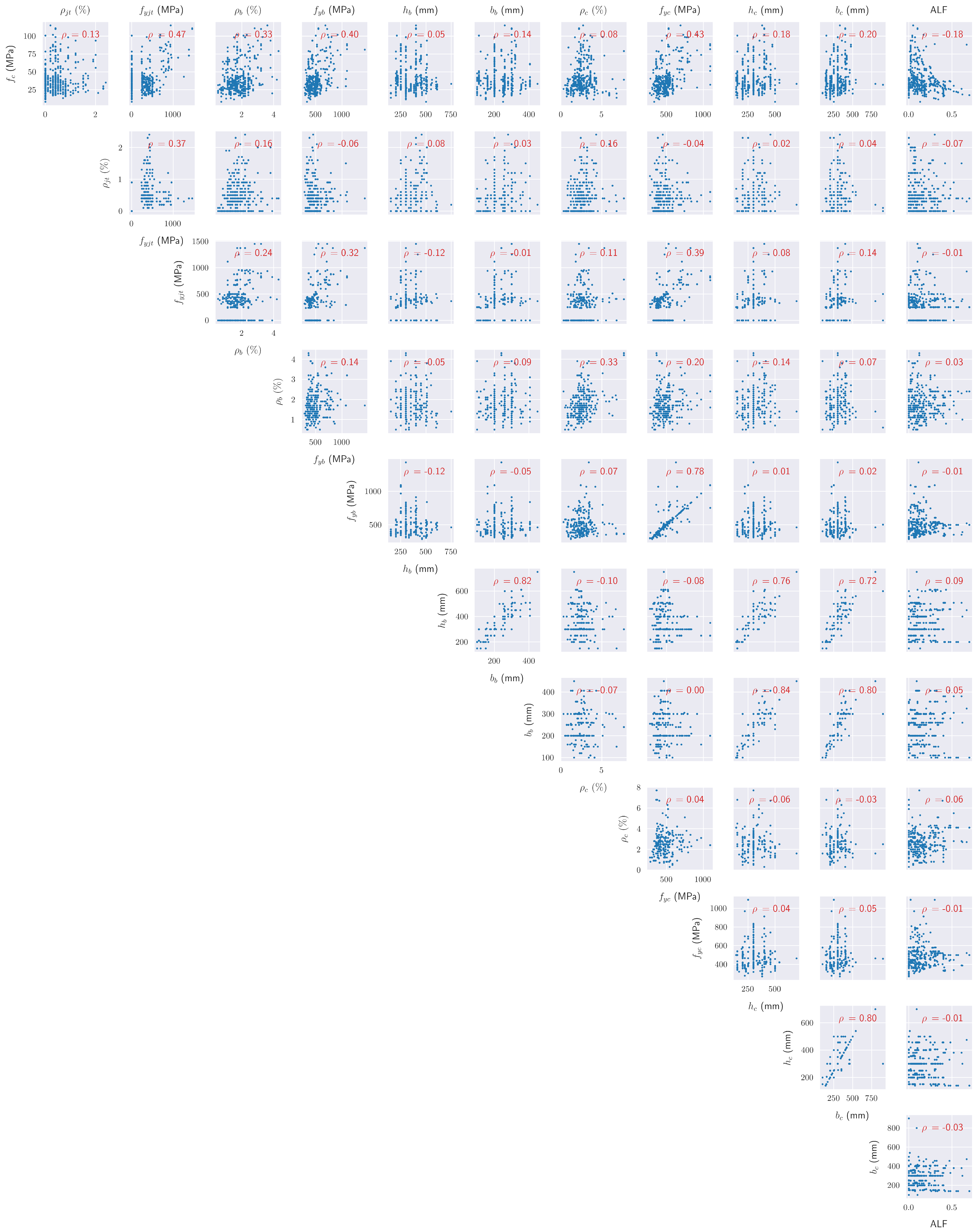
Among the above independent variables, 12 are numeric and describe several geometric and mechanical aspects of the structural elements (joint, beams, and columns), such as their dimensions or their percentage of reinforcement. The last independent variable is categorical and describes the type of the joint, i.e., whether it is interior or exterior. Figure 1 shows the distributions of the target variable and features of the dataset, and Table 1 presents a short description of each one [19]. In addition, Figure 2 provides a pairplot of the independent variables in the dataset. For each pair of variables, each subplot of Figure 2 includes the well-known Pearson’s correlation coefficient ρ . For a pair of variables x , y , this is defined as [25]
ρ x y = i = 1 N ( x i μ x ) ( y i μ y ) σ x σ y ,
where N is the number of points in the dataset, μ x and μ y denote the mean of x and y , while σ x , σ y denote the respective standard deviations.

2.2. Dataset Preprocessing

Dataset preprocessing can involve a variety of different steps that aim to transform the dataset in a form that can be subsequently passed to the machine learning models and improve their performance. In the present study, two such steps were necessitated, as can be observed from Figure 1.
Firstly, it can be observed that two of the variables, namely the joint type and the failure mode, were categorical. In order to transform them into a numerical form suitable for calculations, the one-hot encoding methodology was adopted [26]. Thus, the variable “Joint Type” was assigned a value of 1 if the joint was interior and 0 if the node was exterior. Similarly, the failure mode “JS” was assigned a value of 1 and “BY-JS” was assigned a value of 0.
Secondly, it can be observed that the input features have different orders of magnitude. While this does not affect tree-based ML algorithms, the performance of other models, including Artificial Neural Networks, can be impaired. To this end, several scaling methodologies exist in the literature [27]. In the present study, the so-called StandardScaler was employed, which scales each feature according to the formula
x scaled = x μ σ ,
where x is the value of the feature for a specific input data point, while μ and σ are the feature’s average value and standard deviation, respectively. Thus, this scaling technique centers each feature to have 0 mean and a standard deviation equal to 1.
It should also be noted that the distribution of classes in the target variable, i.e., the failure mode, is balanced. Indeed, approximately 53.7 % of the data points belong to the class “JS” while the remaining 46.7 % belong to the class “BY-JS”, and it can be observed that there is no significant discrepancy between the two. Thus, our dataset does not suffer from the so-called class imbalance problem [28,29], which can adversely affect the performance of any ML model.

3. Machine Learning Algorithms

In this section, we present the theoretical bases of the machine learning algorithms that were employed, before presenting the main findings and results of the present study in the next section.
In this regard, as is mentioned in the Introduction, the focus of the present study is on the so-called ensemble machine learning methodologies. The fundamental principle of ensembling lies in combining the individual strengths of other ML models, called base or individual learners [23], to produce a model with improved performance compared to its constituents. To this end, there exists a variety of well-established classifiers in the ML literature [30]. In the section following, we examine the algorithms that offered the highest accuracy and robustness amongst those considered in our numerical experiments. We first examine the ML models that were employed as base learners, namely Logistic Regression, k-Nearest Neighbors, Decision Tree, and Artificial Neural Networks, which have been successfully implemented individually in engineering applications [17,21,22,31]. Subsequently, we examine how these algorithms were combined using dedicated ensembling methodologies, which is the aim of the present study.

3.1. Individual Learners

As already mentioned, the individual learners that were employed in the present study were Logistic Regression, k-Nearest Neighbors, Decision Tree, and Artificial Neural Networks. In order to harness the benefits of ensembling, these individual learners should be diverse and produce uncorrelated predictions [32,33]. The classifiers selected in the present study work by employing fundamentally different methodologies, thus rendering them suitable candidates for ensembling. To see this, we briefly examine each classifier separately.
  • Logistic Regression (LR): In a binary classification setting, as is the case in the present paper, LR works by solving a linear regression problem on the so-called logit or log-odds [34]. Thus, logistic regression is a linear classifier, as the classification surface it learns corresponds to a hyperplane.
  • k-Nearest Neighbors (k-NN): The fundamental idea behind the k-NN classifier is to assign each input data point x to the majority class of the k “closest” vectors in the training set [35]. These “nearest neighbors” are selected based on a user-defined metric function. The majority can be obtained by simple voting or by weighting the contribution from each individual neighbor.
  • Decision Tree (DT): A Decision Tree generally comprises three parts [36]. The top part is known as the root and corresponds to the initial training dataset. The bottom part comprises the leaves. Between the root and the leaves, the DT contains the branches and the branching nodes. Each node is associated with a single feature/attribute and learns a binary decision rule based on this feature. It is important to note that there is a single path from the root to each leaf [17]. Thus, to classify each data point x , the decision path is followed and x is assigned to the (weighted) majority class of the samples in the corresponding leaf.
  • Artificial Neural Network (ANN): An Artificial Neural Network also generally comprises 3 parts. Each part consists of one or more layers of processing nodes called neurons. The first layer is called the input layer, where the input data points are inserted into the network. The last layer is called the output layer, which produces the final results of the network. In a binary classification setting, this layer consists of a single node, which outputs the probability that the given input vector belongs to the positive class. Between the input and output layers are the so-called hidden layers. Each node in the hidden layers receives as input the output of the nodes in the previous layer and combines them in a weighted sum. Subsequently, this is passed through a so-called activation function, which introduces non-linearities that allow for the model to learn complex patterns in the data.

3.2. Ensemble Methodologies

As previously mentioned, the focus of the present study is on ensemble machine learning methodologies. These combine individual/base models, such as the ones presented in the previous section, to produce a model with increased predictive power. To this end, there are four distinct approaches in the literature, namely (1) bagging, (2) boosting, (3) stacking, and (4) voting [32,33]. We briefly examine each of these methodologies separately.
1.
Bagging: Bagging, which stands for “bootstrap aggregating”, is an ensemble methodology initially introduced by Breiman in 1996 [37]. The fundamental idea behind this algorithm is to use the original training dataset, X train , to produce k new sets, X i = 1 , 2 , . . . , k , by sampling with replacement from X train . These “bootstrapped” datasets are then used to train k corresponding individual learners. Due to the fact that these base models are trained on different datasets, they tend to produce different errors. By aggregating their predictions, these errors tend to cancel each other out, thus improving the overall performance of the ensemble model [37]. Any ML model can be employed as a base model. In fact, in the present study, all the individual learners presented in the previous section were employed as base learners for our bagging ensembles.
2.
Boosting: The individual learners in a boosting ensemble are trained iteratively and sequentially. Each iteration t = 1 , 2 , . . . , T employs a transformed dataset X t * to train the corresponding base learner. The transformed dataset’s target variables are based on the errors of the model up to that iteration. Thus, each successive model iteratively “boosts” the performance of the ensemble [38]. Some widely established boosting algorithms, which were also employed in the present study, include AdaBoost (Adaptive Boosting) [39], Gradient Boosting [38], and XGBoost (eXtreme Gradient Boosting) [40].
3.
Stacking: This ensemble methodology is also known as meta-learning because the predictions of the base models are used to generate the so-called meta-features on which the final ensemble is trained. Optionally, the original features can also be passed as inputs to the ensemble, or they can be combined to create additional meta-features. In order to avoid overfitting, a procedure known as k-fold cross-validation is employed [32,41]. Thus, the training dataset is split into k parts. Iteratively, the algorithm uses k 1 parts to train the base models and the last part is used to generate the predictions, i.e., the meta-features.
4.
Voting: This is arguably the simplest methodology of ensembling. It consists of training a group of models and averaging the predictions. The models are trained independently on the original training dataset X train and not one of its variations, as in the previously examined methodologies. However, this can still offer the advantages of ensembling, as it can provide models that perform better than the individual components [42].
Figure 3 [43] presents some of the above ensemble methodologies for illustration. In the above methodologies, and in fact in all ML models, there are several parameters that are predefined by the user and are not updated during training. These are called the hyperparameters and can include, among others, the maximum allowed depth of each tree, the number of neighbors in k-NN, or the number of maximum iterations in a boosting ensemble. Their selection can affect the model performance and generalization ability. Thus, dedicated methodologies have been proposed to identify the optimal hyperparameter configuration [44]. In the present study, Bayesian Optimization was selected for this task, as it searches the hyperparameter space in an informed manner and, thus, it can converge faster than an exhaustive grid search.
Furthermore, in order to reduce the variance of the obtained classification metrics and, thus, increase their reliability, a so-called nested cross validation scheme was employed [24]. To this end, the dataset is initially split into N parts (in our case, N = 3 ). In an outer loop, each part is iteratively used as a test set to measure the performance of the model on “unseen” data, while the remaining N 1 parts are used as a training set. In an inner loop, these N 1 parts are split into M parts (in our case, M = 2 ) and, similarly, cross validation is performed in order to tune the model hyperparameters. The final performance metrics are the averages from the outer cross validation loop. The ML architectures employed in the study are shown in Table 2.

4. Results

In this Section, we present the main results and findings from the artificial intelligence elaborations conducted in this study to predict the mode of failure of the joints as recorded during the experiments. The performance of the machine learning ensemble methodologies is initially examined. Subsequently, the performance of these models is compared with the predictions obtained by employing the provisions of some of the most widely established seismic design codes.
In order to quantify the performance of the various binary classifiers, Precision, Recall, F1-Score, and Accuracy classification performance metrics were estimated and considered. In binary classification, they are defined as follows [45]:
Precision = TP TP + FP
Recall = TP TP + FN
F 1 - Score = 2 Precision · Recall Precision + Precision
Accuracy = TP + TN TP + TN + FP + FN
In the above equations, TP, FP, FN, and TN denote the number of true positive, false positive, false negative, and true negative input vectors, respectively. It should be clarified that the first three of these metrics are defined for each of the classes separately.
In Figure 4, the comparative results for all these models are presented. As was mentioned in Section 3.2, a nested cross-validation scheme was employed using 3 folds in the outer loop. Thus, all the performance metrics correspond to the aggregated values across the 3 folds, computed on the respective testing set.
From Figure 4, it can be readily observed that all the employed models presented a very good performance on the testing set, with an accuracy of approximately 80% in identifying the joint failure mode. XGBoost obtained the highest overall accuracy of approximately 85%. Gradient Boosting and a bagging ensemble of ANNs also performed very well, with an overall 82.5% success rate in identifying the joint failure mode. However, despite the fact that all the models obtained a high accuracy, there are significant qualitative differences in their behavior, with respect to the other classification metrics. Indeed, for XGBoost, Gradient Boosting, and the bagging ensembles of ANNs, Decision Trees, and Logistic Regression models, the other classification metrics, namely, Precision, Recall, and F1-Score, are all balanced with each other and across the two examined failure modes. This is a desired property because it indicates that the models learned to distinguish the failure modes without developing a bias towards one of them.
On the contrary, AdaBoost, stacking, voting, and the bagging ensemble of k-NNs exhibited a higher variability in their respective performance metrics. On the one hand, AdaBoost obtained a very high Recall for the class “Joint Shear” (“JS”) with a corresponding high Precision for “Beam Yield-Joint Shear” (“BY-JS”). Conversely, its Precision on “JS” and Recall on “BY-JS” were lower. This indicates that this ensemble classifier favored “JS”, as it tried to identify all the correct instances of this class, even at the expense of “BY-JS”. On the other hand, stacking, voting, and the bagging ensemble of k-NNs were more biased towards “BY-JS”. They obtained a high Recall for this class and a corresponding high Precision for “JS”.
In addition, Table 3 presents the corresponding metric values of the best-performing one, XGBoost. These were computed on both the training and testing set, for comparison. It can be readily observed that all the performance metrics are similar to each other and across the two classes. As already mentioned, this indicates that the model is not biased towards one of the two. Similarly, it can be observed that the respective metrics on the training and testing sets are comparable, indicating that the model did not suffer from a severe overfitting effect. The above observations suggest that the model can be confidently employed in practice.
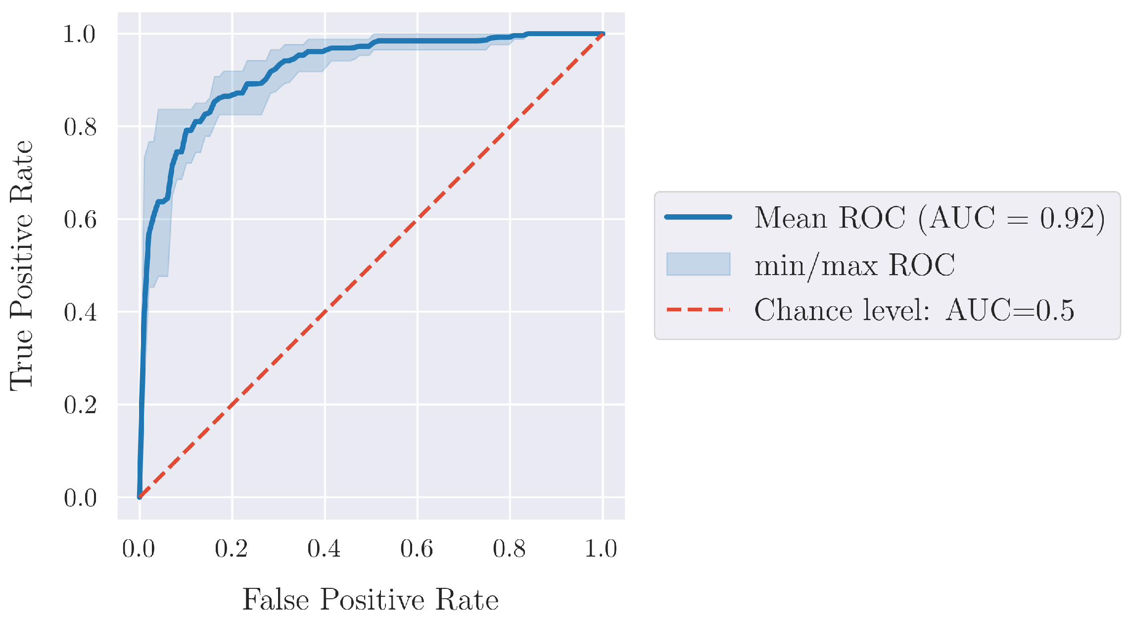
Finally, Figure 5 presents the so-called Receiver Operating Characteristic (ROC) [46] curve for the best-performing classifier, XGBoost. The corresponding Area Under the Curve (AUC) is a measure of the overall performance of the model. It can be readily observed that the model can achieve very high True Positive Rates, i.e., correct predictions, without producing a correspondingly high False Positive Rate. Furthermore, the ROC curves do not exhibit a large variability throughout the cross-validation process.
Subsequently, the performance of the ML models was compared with the predictions of the most widely employed analytical model for the RC joint failure (Park and Paulay [8]), which has been widely adopted by many design codes (ACI [47], New Zealand [48], FIB [49]) and researchers. To obtain the model predictions for the failure mode, the respective load capacities of the beam and the joint were computed. If the capacity of the beam was lower, this indicated that the desirable ductile yielding of the beam occurred prior to joint failure. Thus, in this case, the prediction was set to “BY-JS”. Otherwise, the predicted failure mode was “JS”, since in this case, brittle joint failure due to shear occurs first. The classification metrics based on this model are shown in Table 4, where we also add the classification metrics of XGBoost, for comparison. It can be readily observed that the classification metrics are unbalanced between the two classes. The Recall and F1-Score metrics for the “JS” class are higher than the corresponding metrics for “BY-JS”, indicating that the model has been calibrated towards identifying the brittle, shear failure mode of the RC joint.
As is stated in the Introduction, this failure mode is the most dangerous one due to the qualitative differences in the overall behavior of the system between the two examined failure modes. Specifically, in the “BY-JS” failure mode, a plastic hinge forms in the beam, leading to a flexural, ductile failure mode. However, the beam is still able to absorb seismic energy after this occurs, and the overall stability of the system is not lost. On the other hand, in the case of a “JS” failure mode, the joint fails in a shear, brittle manner. This leads to a sudden loss of stability in the system, after which no further energy can be absorbed, and the system collapses. Local joint collapse may trigger partial or total collapse of the whole structure jeopardizing the protection of the lives of users.
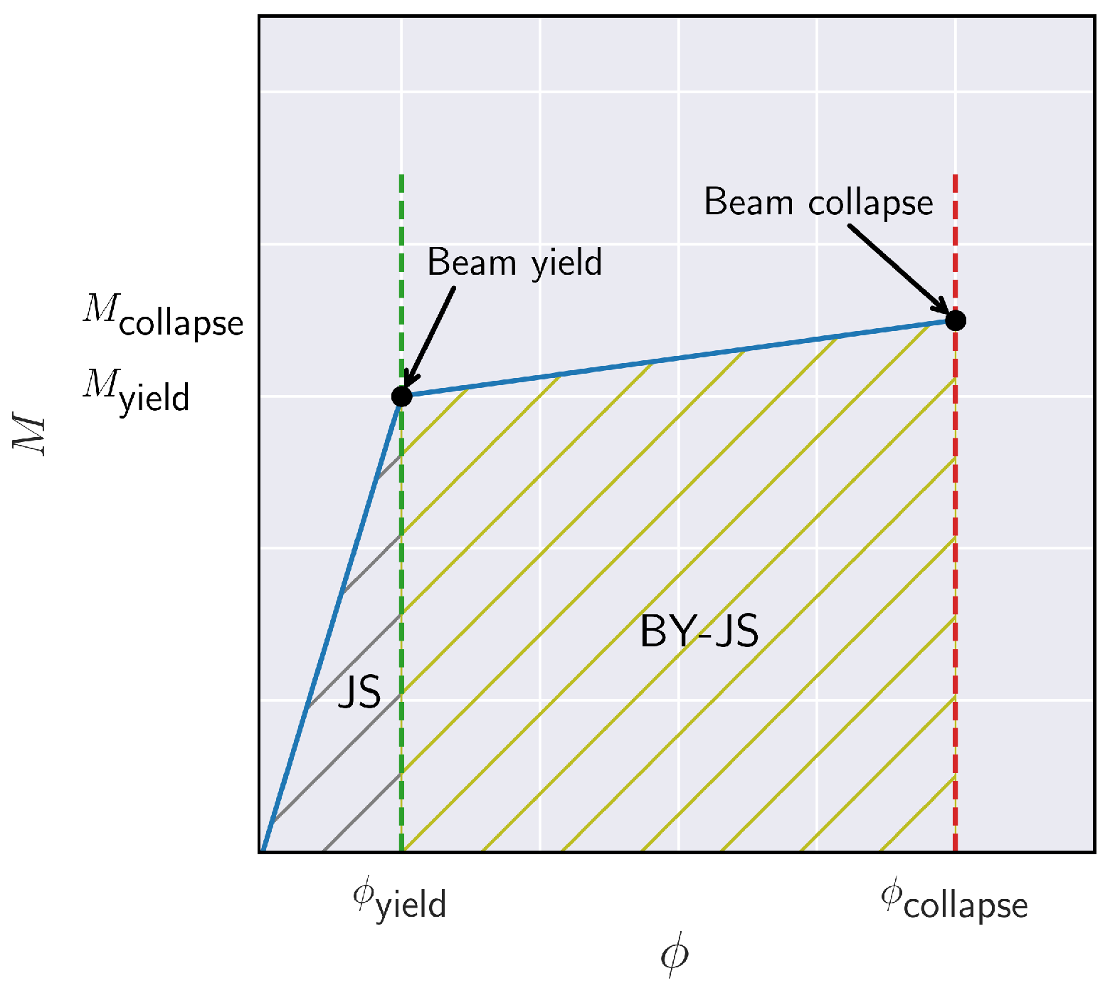
To illustrate the above, we present in Figure 6 an indicative moment–rotation ( M ϕ ) curve for an idealized elastic–plastic beam with hardening. The area under the curve corresponds to the amount of seismic energy that the structural system absorbs. If the joint fails prior to the yielding of the beam, this corresponds to the JS failure mode. Accordingly, if the beam yields prior to the failure of the joint, this corresponds to the BY-JS failure mode. Thus, it can be seen that in the latter case (BY-JS failure mode), the structural system is capable of absorbing larger amounts of seismic energy, which leads to improved performance. On the other hand, if the joint is the first to fail, no further amounts of energy can be absorbed, and the structural system suffers a sudden loss of stability due to brittle shear fracture, contrary to hardening, which does not occur instantaneously.
From Table 4 in conjunction with Figure 4, the benefit of the proposed formulation becomes apparent. Firstly, all the employed ensemble methodologies outperformed the currently established engineering practices. In fact, the accuracy obtained by the most widely employed formula for RC joint failure (Park and Paulay model) was approximately 67%, while all the ensemble methodologies obtained an accuracy approximately 12–18% higher. Furthermore, the best-performing classifier, XGBoost, obtained a significantly more balanced performance between the two classes. Indeed, as was mentioned, the Park and Paulay model exhibited higher performance metrics for the “JS” class. This indicates that the model is calibrated to favor the identification of the brittle “JS” failure mode. On the other hand, the corresponding difference in the metrics of XGBoost ranged between 1 and 3%. Thus, the performance of the model was more balanced between the two classes and exhibited less bias.
This is an improvement over similar studies in the literature. For example, the authors in [21] obtained an overall accuracy of approximately 81.8 % with the best examined classifier examined therein, i.e., LASSO Logistic Regression. The reported Recall index for the BY-JS failure mode ranged from approximately 64.4 % (Random Forest) to 76.3 % (k-Nearest Neighbors). Similarly, for the JS failure mode, the respective metric ranged from approximately 88.1 % (Discriminant Analysis and Support Vector Machine) to 94.1 % (LASSO Logistic Regression and Random Forest). The respective differences between the metrics of the two failure modes ranged from approximately 12.8 % (k-Nearest Neighbors) to 29.6 % (Random Forest). Thus, the models proposed in the present study obtained a higher overall accuracy and much smaller deviations between the respective metrics of the two failure modes, indicating a more balanced performance that is not biased towards one of the two modes.

5. Summary and Conclusions

One of the most critical aspects of the seismic behavior of a reinforced concrete structure pertains to the joints between beams and their adjacent columns. Joint failure, especially in structures adhering to older design codes, is often due to shear and brittle (“Joint Shear”-“JS” failure mode). In turn, this can lead to a partial or total collapse of the structure and loss of human lives. On the other hand, the desired mechanical behavior as described by the provisions of modern design codes considers the ductile failure mode “Beam Yield-Joint Shear” (“BY-JS”) to be more favorable. In this scenario, during a major earthquake, ductile failure/yielding of the beam occurs prior to joint failure.
This allows for the RC frame as whole, as well as its individual sub-systems, to develop larger deformations during major seismic events before their capacity is lost. Furthermore, the overall stability remains satisfactory. Finally, the structure is able to absorb larger amounts of energy during the earthquake, which simultaneously increases the available evacuation time. Thus, one of the most impactful and complex engineering challenges is to estimate the joint failure mode for a large number of structures in a given building stock.
To this end, in the framework of the present study, ML classification algorithms were employed for this task. Emphasis was given to ensemble techniques, which combine individual/base models to produce the final classifier. Specifically, the four most common ensemble methodologies were used, namely stacking, boosting, voting, and bagging. For each methodology, experiments were conducted by employing not only different ML models as individual learners, but also different ensemble architectures, as shown in Table 2. The performance of the models was measured using well-known classification metrics, namely Accuracy, Precision, Recall, and F1-Score. Furthermore, a nested cross-validation scheme was employed, which reduced the variance of the extracted classification metrics and increased the generalization potential of the developed models. The performance of the employed methodologies was compared against the results obtained by the Park and Paulay model, which is widely adopted by various international seismic design codes and researchers.
As it can be observed from Table 4 and Figure 4, in the examined case, all the employed methodologies significantly outperformed the aforementioned model. Some models, for example AdaBoost, stacking, voting, and the bagging ensemble of k-NNs, exhibited a higher variability in their classification metrics. This indicated that these models were slightly biased towards one of the two classes. However, as it can be observed from Table 3, the best-performing classifier, XGBoost, exhibited only a small variability among its various performance metrics, indicating that the model is unbiased and can be confidently employed in practice.
Overall, the results of the present study are promising and encourage the potential applicability of such methods to tackle the problem of beam–column joints failure mode prediction, as well as similar complex and impactful engineering challenges. Finally, even though our numerical experimentations were based on a dataset comprising 486 RC joint specimens, the employed methodologies can be continuously updated as new data become available. This can potentially allow for more complex models to be trained, while mitigating the risk of overfitting on one particular dataset.

Author Contributions

Conceptualization, M.K., I.K., T.R., L.I. and A.K.; methodology, M.K., I.K., T.R., L.I. and A.K.; software, M.K., I.K., T.R., L.I. and A.K.; validation, M.K., I.K., T.R., L.I. and A.K.; formal analysis, M.K. and I.K.; investigation, M.K., I.K., T.R., L.I. and A.K.; resources, M.K., T.R. and L.I.; data curation, M.K., I.K., T.R., L.I. and A.K.; writing—original draft preparation, M.K. and I.K.; writing—review and editing, T.R., L.I. and A.K; visualization, M.K. and I.K.; supervision T.R., L.I. and A.K. All authors have read and agreed to the published version of the manuscript.

Funding

This research received no external funding.

Institutional Review Board Statement

Not applicable.

Informed Consent Statement

Not applicable.

Data Availability Statement

The data that support the findings of this study are available upon reasonable request.

Conflicts of Interest

The authors declare no conflicts of interest.

Abbreviations

The following abbreviations are used in this manuscript:
RCReinforced Concrete
MLMachine Learning
ANNArtificial Neural Network
OLSOrdinary Least Squares
SVMSupport Vector Machine
MARSMultivariate Adaptive Regression Splines
ELMExtreme Learning Machine
DTDecision Tree
XGBoosteXtreme Gradient Boosting

References

  1. Palermo, V.; Tsionis, G.; Sousa, M.L. Building Stock Inventory to Assess Seismic Vulnerability Across Europe; Technical Report; Publications Office of the European Union: Luxembourg, 2018. [Google Scholar]
  2. Pantelides, C.P.; Hansen, J.; Ameli, M.; Reaveley, L.D. Seismic performance of reinforced concrete building exterior joints with substandard details. J. Struct. Integr. Maint. 2017, 2, 1–11. [Google Scholar] [CrossRef]
  3. Najafgholipour, M.; Dehghan, S.; Dooshabi, A.; Niroomandi, A. Finite element analysis of reinforced concrete beam-column connections with governing joint shear failure mode. Lat. Am. J. Solids Struct. 2017, 14, 1200–1225. [Google Scholar] [CrossRef]
  4. Kuang, J.; Wong, H. Behaviour of Non-seismically Detailed Beam-column Joints under Simulated Seismic Loading: A Critical Review. In Proceedings of the fib Symposium on Concrete Structures: The Challenge of Creativity, Avignon, France, 26–28 May 2004. [Google Scholar]
  5. Karayannis, C.G.; Sirkelis, G.M. Strengthening and rehabilitation of RC beam–column joints using carbon-FRP jacketing and epoxy resin injection. Earthq. Eng. Struct. Dyn. 2008, 37, 769–790. [Google Scholar] [CrossRef]
  6. Karabinis, A.; Rousakis, T. Concrete confined by FRP material: A plasticity approach. Eng. Struct. 2002, 24, 923–932. [Google Scholar] [CrossRef]
  7. Tsonos, A.; Stylianidis, K. Pre-seismic and post-seismic strengthening of reinforced concrete structural subassemblages using composite materials (FRP). In Proceedings of the 13th Hellenic Concrete Conference, Rethymno, Greece, 25 October 1999; Volume 1, pp. 455–466. [Google Scholar]
  8. Park, R.; Paulay, T. Reinforced Concrete Structures; John Wiley & Sons: Hoboken, NJ, USA, 1991. [Google Scholar]
  9. Tsonos, A.G. Cyclic load behaviour of reinforced concrete beam-column subassemblages of modern structures. WIT Trans. Built Environ. 2005, 81, 439–449. [Google Scholar]
  10. Antonopoulos, C.P.; Triantafillou, T.C. Experimental investigation of FRP-strengthened RC beam-column joints. J. Compos. Constr. 2003, 7, 39–49. [Google Scholar] [CrossRef]
  11. Karayannis, C.; Golias, E.; Kalogeropoulos, G.I. Influence of carbon fiber-reinforced ropes applied as external diagonal reinforcement on the shear deformation of RC joints. Fibers 2022, 10, 28. [Google Scholar] [CrossRef]
  12. Karabini, M.; Rousakis, T.; Golias, E.; Karayannis, C. Seismic tests of full scale reinforced concrete T joints with light external continuous composite rope strengthening—Joint deterioration and failure assessment. Materials 2023, 16, 2718. [Google Scholar] [CrossRef]
  13. Nikolić, Ž.; Živaljić, N.; Smoljanović, H.; Balić, I. Numerical modelling of reinforced-concrete structures under seismic loading based on the finite element method with discrete inter-element cracks. Earthq. Eng. Struct. Dyn. 2017, 46, 159–178. [Google Scholar] [CrossRef]
  14. Ghobarah, A.; Biddah, A. Dynamic analysis of reinforced concrete frames including joint shear deformation. Eng. Struct. 1999, 21, 971–987. [Google Scholar] [CrossRef]
  15. Thai, H.T. Machine learning for structural engineering: A state-of-the-art review. Structures 2022, 38, 448–491. [Google Scholar] [CrossRef]
  16. Karampinis, I.; Iliadis, L. Seismic vulnerability of reinforced concrete structures using machine learning. Earthquakes Struct. 2024, 27, 83. [Google Scholar]
  17. Karampinis, I.; Bantilas, K.E.; Kavvadias, I.E.; Iliadis, L.; Elenas, A. Machine Learning Algorithms for the Prediction of the Seismic Response of Rigid Rocking Blocks. Appl. Sci. 2023, 14, 341. [Google Scholar] [CrossRef]
  18. Kotsovou, G.M.; Cotsovos, D.M.; Lagaros, N.D. Assessment of RC exterior beam-column Joints based on artificial neural networks and other methods. Eng. Struct. 2017, 144, 1–18. [Google Scholar] [CrossRef]
  19. Suwal, N.; Guner, S. Plastic hinge modeling of reinforced concrete Beam-Column joints using artificial neural networks. Eng. Struct. 2024, 298, 117012. [Google Scholar] [CrossRef]
  20. Marie, H.S.; Abu El-hassan, K.; Almetwally, E.M.; El-Mandouh, M.A. Joint shear strength prediction of beam-column connections using machine learning via experimental results. Case Stud. Constr. Mater. 2022, 17, e01463. [Google Scholar] [CrossRef]
  21. Mangalathu, S.; Jeon, J.S. Classification of failure mode and prediction of shear strength for reinforced concrete beam-column joints using machine learning techniques. Eng. Struct. 2018, 160, 85–94. [Google Scholar] [CrossRef]
  22. Gao, X.; Lin, C. Prediction model of the failure mode of beam-column joints using machine learning methods. Eng. Fail. Anal. 2021, 120, 105072. [Google Scholar] [CrossRef]
  23. Rincy, T.N.; Gupta, R. Ensemble learning techniques and its efficiency in machine learning: A survey. In Proceedings of the 2nd International Conference on Data, Engineering and Applications (IDEA), Bhopal, India, 28–29 February 2020; pp. 1–6. [Google Scholar]
  24. Scheda, R.; Diciotti, S. Explanations of machine learning models in repeated nested cross-validation: An application in age prediction using brain complexity features. Appl. Sci. 2022, 12, 6681. [Google Scholar] [CrossRef]
  25. Ma, C.; Chi, J.w.; Kong, F.c.; Zhou, S.h.; Lu, D.c.; Liao, W.z. Prediction on the seismic performance limits of reinforced concrete columns based on machine learning method. Soil Dyn. Earthq. Eng. 2024, 177, 108423. [Google Scholar] [CrossRef]
  26. Al-Shehari, T.; Alsowail, R.A. An insider data leakage detection using one-hot encoding, synthetic minority oversampling and machine learning techniques. Entropy 2021, 23, 1258. [Google Scholar] [CrossRef] [PubMed]
  27. Ahsan, M.M.; Mahmud, M.P.; Saha, P.K.; Gupta, K.D.; Siddique, Z. Effect of data scaling methods on machine learning algorithms and model performance. Technologies 2021, 9, 52. [Google Scholar] [CrossRef]
  28. Abd Elrahman, S.M.; Abraham, A. A review of class imbalance problem. J. Netw. Innov. Comput. 2013, 1, 9. [Google Scholar]
  29. Longadge, R.; Dongre, S. Class imbalance problem in data mining review. arXiv 2013, arXiv:1305.1707. [Google Scholar]
  30. Kotsiantis, S.B.; Zaharakis, I.; Pintelas, P. Supervised machine learning: A review of classification techniques. Emerg. Artif. Intell. Appl. Comput. Eng. 2007, 160, 3–24. [Google Scholar]
  31. Aloisio, A.; Rosso, M.M.; Di Battista, L.; Quaranta, G. Machine-learning-aided regional post-seismic usability prediction of buildings: 2016–2017 Central Italy earthquakes. J. Build. Eng. 2024, 91, 109526. [Google Scholar] [CrossRef]
  32. Ganaie, M.A.; Hu, M.; Malik, A.K.; Tanveer, M.; Suganthan, P.N. Ensemble deep learning: A review. Eng. Appl. Artif. Intell. 2022, 115, 105151. [Google Scholar] [CrossRef]
  33. Dietterich, T.G. Ensemble methods in machine learning. In International Workshop on Multiple Classifier Systems; Springer: Berlin/Heidelberg, Germany, 2000; pp. 1–15. [Google Scholar]
  34. Algamal, Z.Y.; Lee, M.H. Regularized logistic regression with adjusted adaptive elastic net for gene selection in high dimensional cancer classification. Comput. Biol. Med. 2015, 67, 136–145. [Google Scholar] [CrossRef]
  35. Steinbach, M.; Tan, P.N. kNN: k-nearest neighbors. In The Top Ten Algorithms in Data Mining; Chapman and Hall/CRC: London, UK, 2009; pp. 165–176. [Google Scholar]
  36. Loh, W.Y. Classification and regression trees. Wiley Interdiscip. Rev. Data Min. Knowl. Discov. 2011, 1, 14–23. [Google Scholar] [CrossRef]
  37. Breiman, L. Bagging predictors. Mach. Learn. 1996, 24, 123–140. [Google Scholar] [CrossRef]
  38. Friedman, J.H. Greedy function approximation: A gradient boosting machine. Ann. Stat. 2001, 29, 1189–1232. [Google Scholar] [CrossRef]
  39. Freund, Y.; Schapire, R.E. A decision-theoretic generalization of on-line learning and an application to boosting. J. Comput. Syst. Sci. 1997, 55, 119–139. [Google Scholar] [CrossRef]
  40. Chen, T.; Guestrin, C. Xgboost: A scalable tree boosting system. In Proceedings of the 22nd ACM Sigkdd International Conference on Knowledge Discovery and Data Mining, San Francisco, CA, USA, 13–17 August 2016; pp. 785–794. [Google Scholar]
  41. Wolpert, D.H. Stacked generalization. Neural Netw. 1992, 5, 241–259. [Google Scholar] [CrossRef]
  42. Leon, F.; Floria, S.A.; Bădică, C. Evaluating the effect of voting methods on ensemble-based classification. In Proceedings of the 2017 IEEE International Conference on Innovations in Intelligent Systems and Applications (INISTA), Gdynia, Poland, 3–5 July 2017; pp. 1–6. [Google Scholar]
  43. Karampinis, I. Mathematical Structure of Fuzzy Connectives with Applications in Artificial Intelligence. PhD Thesis, Democritus University of Thrace, Komotini, Greece, 2024. [Google Scholar]
  44. Yang, L.; Shami, A. On hyperparameter optimization of machine learning algorithms: Theory and practice. Neurocomputing 2020, 415, 295–316. [Google Scholar] [CrossRef]
  45. Raschka, S. An overview of general performance metrics of binary classifier systems. arXiv 2014, arXiv:1410.5330. [Google Scholar]
  46. Fan, J.; Upadhye, S.; Worster, A. Understanding receiver operating characteristic (ROC) curves. Can. J. Emerg. Med. 2006, 8, 19–20. [Google Scholar] [CrossRef]
  47. Recommendations for Design of Beam-Column Connections in Monolithic Reinforced Concrete Structures (ACI 352R-02); Technical Report; Amercian Concrete Institute: Indianapolis, IN, USA, 2002.
  48. Liu, A.; Park, R. Seismic behavior and retrofit of pre-1970’s as-built exterior beam-column joints reinforced by plain round bars. Bull. N. Z. Soc. Earthq. Eng. 2001, 34, 68–81. [Google Scholar] [CrossRef]
  49. Retrofitting of Concrete Structures by Externally Bonded FRPs with Emphasis on Seismic Applications (FIB-35); Technical Report; The International Federation for Structural Concrete: Lausanne, Switzerland, 2002.
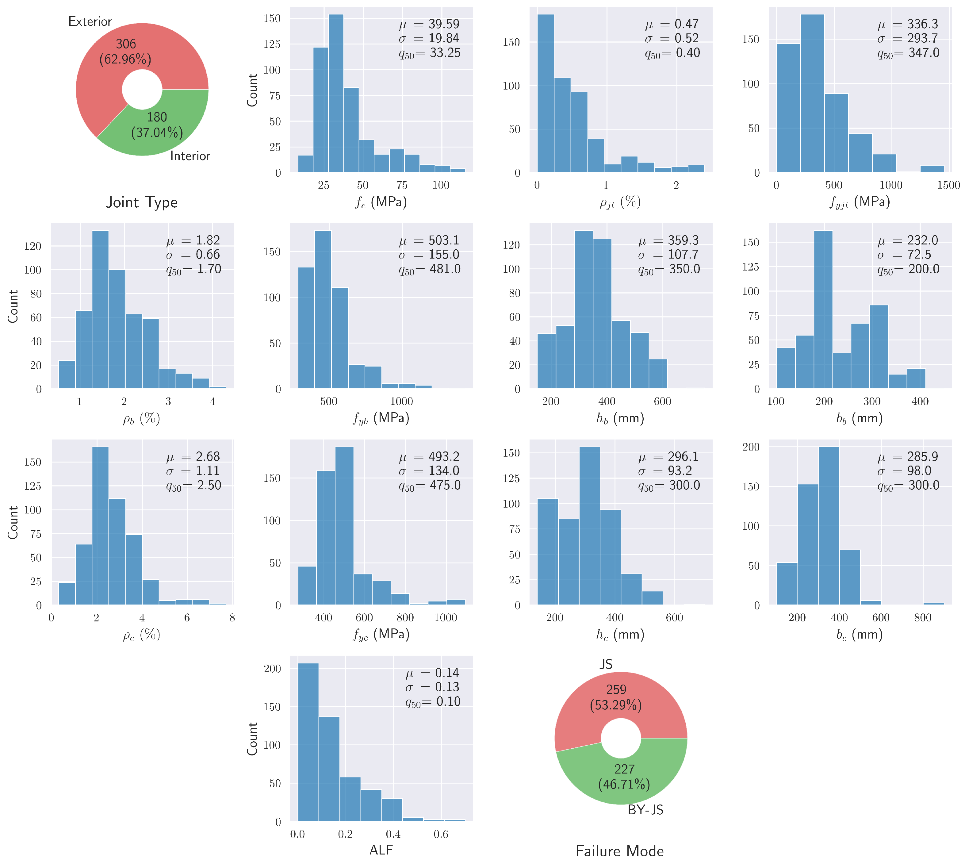
Figure 1. Distributions and descriptive statistics of the features and target variable. In the above, μ , σ , and q 50 correspond to the mean, standard deviation, and median, respectively.
Information 15 00647 g001
Figure 2. Pairplot of the independent variables in the dataset. In each subplot, ρ corresponds to the Pearson correlation coefficient defined in Equation (1).
Information 15 00647 g002
Figure 3. Illustration of ensemble methodologies. (a) Bagging, (b) boosting, and (c) stacking [43]. In the above, X t * , t = 1 , 2 , . . . , T , are the transformed training datasets examined in the previous paragraphs.
Information 15 00647 g003
Figure 4. Comparison of the cross-validated performance metrics of the ensembles.
Information 15 00647 g004
Figure 5. ROC curve for the best-performing classifier, XGBoost.
Information 15 00647 g005
Figure 6. Indicative moment–rotation ( M ϕ ) curve for an idealized elastic–plastic beam with hardening. The area under the curve corresponds to the amount of seismic energy that the structural system absorbs.
Information 15 00647 g006
Table 1. Description of the independent variables [19].
FeatureDescription
f c (MPa)The compressive strength of the concrete.
ρ jt The percentage of transverse reinforcement (stirrups) in the joint.
f yjt (MPa)The yield stress of the stirrups in the joint.
ρ b (%)The percentage of longitudinal reinforcement in the beam.
f yb (MPa)The yield stress of the longitudinal reinforcement in the beam.
h b (mm), b b (mm)The height and width of the beam, respectively.
ρ c (%)The percentage of longitudinal reinforcement in the column.
f yc (MPa)The yield stress of the longitudinal reinforcement in the column.
h c (mm), b c (mm)The height and width of the column, respectively.
ALF (%)The axial load factor.
Table 2. Description of the ensemble architectures.
EnsembleArchitecture Description
BaggingEach of the Logistic Regression, k-Nearest Neighbors, Decision Tree, and ANN was independently employed as a base model for the bagging ensemble.
BoostingAdaBoost, XGBoost, and Gradient Boosting were implemented separately.
StackingLogistic Regression, k-Nearest Neighbors, and Decision Tree were used as base learners. ANN was used as the final meta-model.
VotingLogistic Regression, k-Nearest Neighbors, Decision Tree, and ANN were employed as base learners.
Table 3. Performance metrics of the best performing classifier, XGBoost.
Training SetTesting Set
BY-JSJSBY-JSJS
Precision0.920860.930460.835780.86361
Recall0.920720.930490.845780.85311
F1-Score0.920760.930450.840360.85801
Accuracy0.925930.84979
Table 4. Performance metrics based on the Park and Paulay model [8], compared with the best-performing classifier, XGBoost.
Park and PaulayXGBoost
BY-JSJSBY-JSJS
Precision0.707010.647420.835780.86361
Recall0.488980.822390.845780.85311
F1-Score0.578130.724490.840360.85801
Accuracy0.666670.84979
Disclaimer/Publisher’s Note: The statements, opinions and data contained in all publications are solely those of the individual author(s) and contributor(s) and not of MDPI and/or the editor(s). MDPI and/or the editor(s) disclaim responsibility for any injury to people or property resulting from any ideas, methods, instructions or products referred to in the content.