Three-Stage MPViT-DeepLab Transfer Learning for Community-Scale Green Infrastructure Extraction

Abstract

The extraction of community-scale green infrastructure (CSGI) poses challenges due to limited training data and the diverse scales of the targets. In this paper, we reannotate a training dataset of CSGI and propose a three-stage transfer learning method employing a novel hybrid architecture, MPViT-DeepLab, to help us focus on CSGI extraction and improve its accuracy. In MPViT-DeepLab, a Multi-path Vision Transformer (MPViT) serves as the feature extractor, feeding both coarse and fine features into the decoder and encoder of DeepLabv3+, respectively, which enables pixel-level segmentation of CSGI in remote sensing images. Our method achieves state-of-the-art results on the reannotated dataset.

1. Introduction

Urban green space (UGS) refers to natural environment areas within urban areas, which typically comprise natural elements, such as trees, grass, gardens, parks, forests, lakes, rivers, lawns, and more. These green spaces can be located in various parts of the city, including downtown areas, communities, residential neighborhoods, and industrial zones. The extraction of urban green spaces can be achieved through traditional methods [1,2] as well as deep learning-based approaches [3,4]. In [5], the concept of community-scale green infrastructure (CSGI) is introduced and pertains to public facilities built to promote community sustainability. Compared to urban green spaces, these infrastructures are smaller in scale. CSGI extraction is of significant value for community planning, landscaping, and sustainable development. In this paper, we categorize CSGI into five classes based on their specific functions within the community: Grass, Tree, Bush area, Lake, and Terrace greenery, which collectively cover over 90 percent of the green infrastructure within the community.

CSGI extraction is a remote sensing semantic segmentation task. Semantic segmentation in remote sensing imagery has long been one of the challenging problems in the field of computer vision. This difficulty arises from the significant variations in the appearance of segmented objects and the irregular spatial distribution. Convolutional neural networks (CNNs), as excellent feature extractors, have been widely applied to remote sensing image segmentation tasks [6,7]. However, conventional CNNs for classification often incorporate consecutive pooling and downsampling operations, leading to a decrease in spatial resolution and a limitation in modeling long-range dependencies. To address this issue, researchers have attempted to improve the network structure of CNNs. For instance, U-Net [8], with its encoder–decoder structure and skip connections, performs well in medical image segmentation [9] and remote sensing image segmentation tasks and achieves promising results in building extraction [10,11]. To give another example, the DeepLab series of networks [12,13,14,15] increases kernel sizes, employs atrous convolutions, and establishes spatial pyramids to expand the receptive field for pixel-level image segmentation. These optimizations enhance the long-range dependency of feature maps.

The Transformer architecture originally gained tremendous success in the field of natural language processing by stacking multi-head attention modules to model long-range dependencies, effectively compensating for the limitations of CNN. As a result, the Vision Transformer (ViT) [16] processes images in the form of token sequences, similar to dealing with natural language. However, it has a significant drawback in that it requires large amounts of data and long training times to match the performance of CNNs. The Swin Transformer [17] introduces the concept of a mobile window to make ViT more efficient. The Multi-path Vision Transformer (MPViT) [18] takes a different approach by constructing parallel multi-path structures, simultaneously utilizing the non-local connectivity of convolution and the end-to-end dependency of Transformer, which allows it to represent fine and coarse features for dense prediction tasks effectively.

CSGI extraction requires attention to both global and local features. Additionally, the dense and overlapping distribution of segmentation objects in CSGI, coupled with the difficulty of manual labeling and the scarcity of training data, poses significant challenges for extraction. The lack of training data and the introduction of new extraction targets led us to consider transfer learning. Early on, transfer learning found extensive applications in multi-task learning [19] and domain adaptation [20]. With the rise of deep learning in the 21st century, researchers have begun to use transfer learning to tackle more complex tasks and data. Jason Yosinski and his colleagues [21], through experimentation and trials, provide substantial support and affirmation for the transferability of deep networks. When transfer learning is appropriately employed, the accuracy of deep learning tasks can be significantly improved while reducing training time. Transfer learning has found numerous applications in fields such as medicine [22,23], industry [24], finance [25,26], biology [27], music [28], environment [29], and computer vision [30,31].

In this paper, we use DeepLabv3+ as the backbone network to compare the segmentation performance of Mobilenet [32], Resnet101 [33], Xception [34], and MPViT as a feature extraction network on CSGI. Additionally, we investigate which batch normalization (BN) layers of MPViT-DeepLab should be frozen during the three-stage transfer learning process. In summary, the contributions of this paper are as follows:

• We reannotate a dataset suitable for training in the task of CSGI extraction.
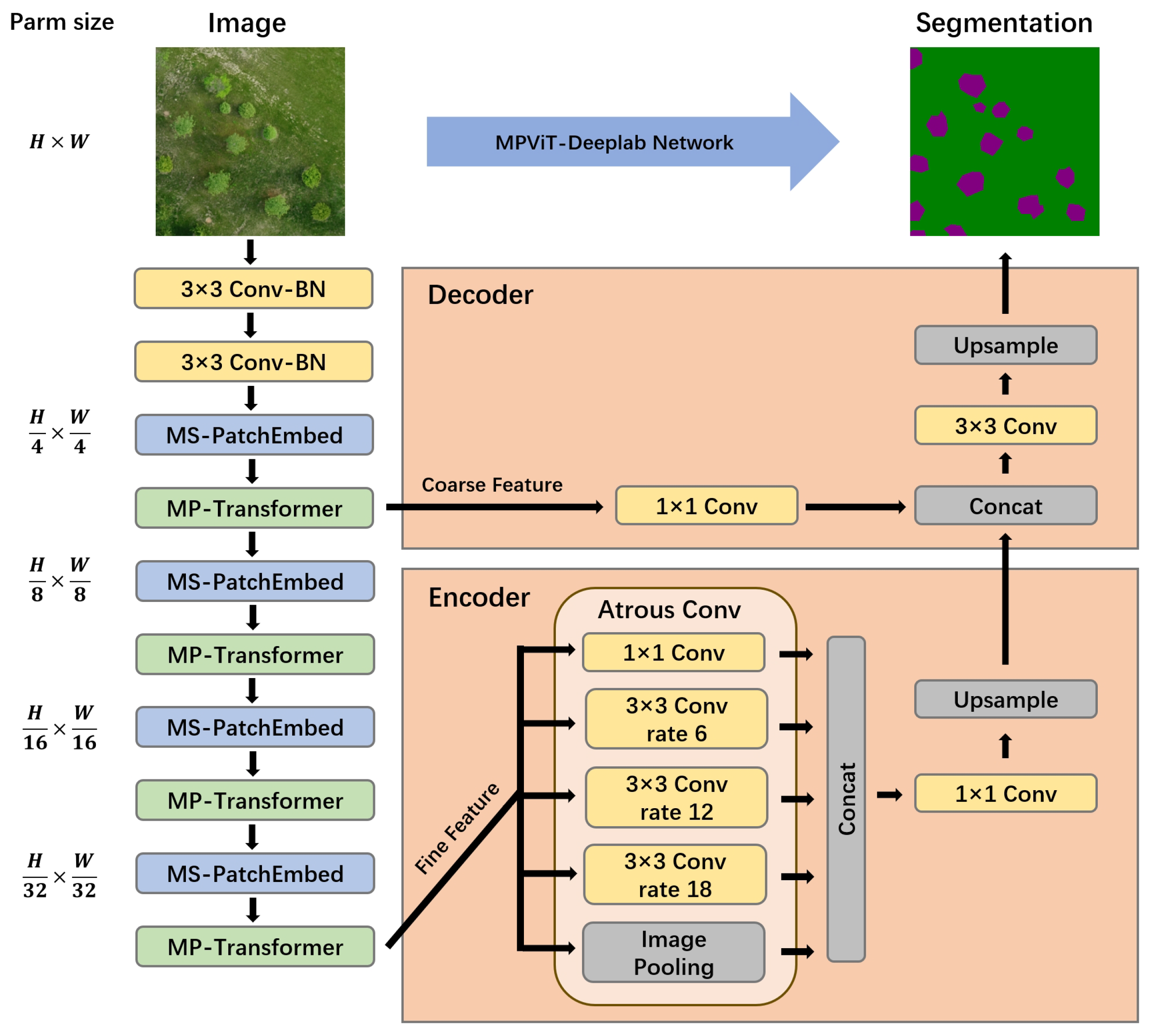
• We feed the coarse and fine features extracted by MPViT into DeepLabv3+ for pixel-level segmentation of CSGI in the three-stage transfer learning process.
• We confirm that three-stage MPViT-DeepLab transfer learning, along with freezing all BN layers during the second transfer learning, achieves state-of-the-art performance in the CSGI extraction task on the reannotate dataset.

2. Related Work

The hybrid architecture we employ, MPViT-DeepLab, utilizes DeepLabv3+ as the backbone with MPViT serving as the feature extractor. In this section, we will provide a detailed explanation of the specific configurations of the MPViT and DeepLabv3+ that we use.

2.1. Multi-Path Vision Transformer

In [18], the Multi-path Vision Transformer (MPViT) is primarily constructed using a Multi-Scale PatchEmbed (MS-PatchEmbed) block and a Multi-Path Transformer (MP-Transformer) block to build a parallel multi-path structure, capturing both fine and coarse features for dense prediction tasks. Figure 1 provides a specific illustration of the MPViT network architecture. We input an image of dimensions $H\times W\times 3$. Initially, the image undergoes two consecutive convolutional batch normalization (Conv-BN) layers with a $3\times 3$ convolution kernel and a stride of 2, which serve to reduce dimensionality and model parameters. After this stage, the feature size becomes $\frac{H}{4}\times \frac{W}{4}\times C^{\prime }$, where C’ represents the channel size for the next stage. The Conv-BN layer consists of a convolutional layer, a batch normalization layer, and a Handswish activation function. Following this, the process involves four iterations, each consisting of an MS-PatchEmbed block and an MP-Transformer block. The MS-PatchEmbed block can extract image sequences of different sizes using depth-wise convolution, while the MP-Transformer block processes the image sequences passed by the MS-PatchEmbed block through a Transformer Encoder, resulting in the aggregation of local and global features. In the following sections, we will provide a detailed description of each component.

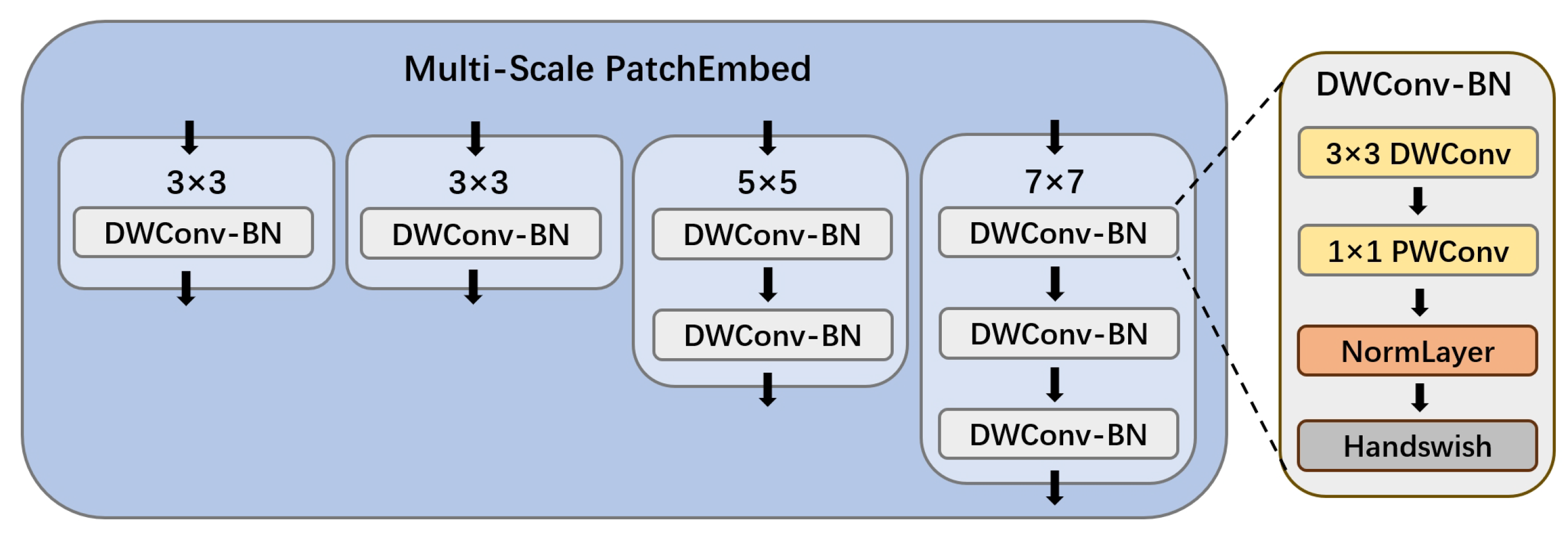
2.1.1. Multi-Scale PatchEmbed Block

The Multi-Scale PatchEmbed block’s specific content is illustrated in Figure 2. It designs a function $F_{k\times k}(·)$, which employs convolution with overlapping patches. $F_{k\times k}(·)$ represents a 2D convolution operation with a kernel size of $k\times k$, stride s, and padding p. When $F(·)$ is given a set of features $X_i\in {\mathbb{R}}^{H_{i-1}\times W_{i-1}\times C_{i-1}}$ as input, the calculation of the resulting $F_{k\times k}\left(X_i\right)\in {\mathbb{R}}^{H_i\times W_i\times C_i}$ in terms of height $H_i$ and width $W_i$ is as follows:

$$H_i=⌊\frac{H_{i-1}-k+2p}{s}+1⌋,W_i=⌊\frac{W_{i-1}-k+2p}{s}+1⌋$$

(1)

By adjusting the sizes of k, s, and p, we can determine whether to generate features of the same size or reduce spatial resolution. When $s=1$ and $p=⌊\frac{k-1}{2}⌋$, we can use batches of different sizes to generate features of the same size. The $H\times W\times C$ image features, regardless of whether they pass through $3\times 3$, $5\times 5$, or $7\times 7$ convolutions, will not change the H and W sizes. This allows visual tokens of the same sequence length to be passed into the Transformer Encoder. When we need to reduce spatial resolution, we increase the stride, such as when $s=2$, which reduces the spatial resolution to half of its original value. Within each Multi-Scale PatchEmbed block, we perform two convolutions with $s=2$. For instance, given the feature size $X_i\in {\mathbb{R}}^{H_i\times W_i\times C_i}$, in the next stage, the input feature size becomes $X_{i+1}\in {\mathbb{R}}^{\frac{H_{i+1}}{4}\times \frac{W_{i+1}}{4}\times C_{i+1}}$.

Stacking convolution blocks allows us to achieve the same receptive field as a larger kernel with fewer parameters. As a result, our $5\times 5$ convolution is composed of two $3\times 3$ convolutions ($2\times 3^2<5^2$), and similarly, our $7\times 7$ convolution is formed by stacking three $3\times 3$ convolutions ($3\times 3^2<7^2$). The depthwise separable convolutions [34] (depicted as DWConv-BN in Figure 3) consist of a $3\times 3$ depthwise convolution and a $1\times 1$ pointwise convolution, followed by a batch normalization layer [35] and a Handswish activation function [36].

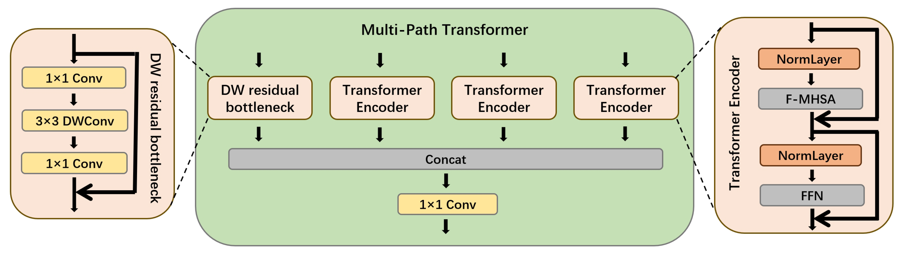
2.1.2. Multi-Path Transformer Block

The structure of the multi-path Transformer block is depicted in Figure 3. The purpose of the multi-path Transformer block is to capture long-range dependencies while paying attention to local feature relationships. It mainly comprises two types of modules: the Depthwise Residual Bottleneck block (DW Residual Bottleneck) and the Transformer Encoder block. The DW Residual Bottleneck block consists of a $1\times 1$ convolution, a $3\times 3$ depthwise convolution, and another $1\times 1$ convolution [33]. Its primary role is to extract local features with a relatively lower parameter count and computational cost in both spatial and channel dimensions. Within the Transformer Encoder block, efficient factorized self-attention [37] is employed (depicted as the F-MHSA block in Figure 4) to alleviate the computational burden:

$$\mathrm{FactorAtt}(Q,K,V)=\frac{Q}{\sqrt{C}}\left(\mathrm{softmax}{\left(K\right)}^{\top }V\right),$$

(2)

where $Q,K,V\in {\mathbb{R}}^{N\times C}$ represent linearly projected queries, keys, and values, and N, C denote tokens and channels. Due to the self-attention mechanism of the Transformer and its ability to disregard position and sequence size, it exhibits great strength in handling global features. The Transformer Encoder block is capable of extracting global features in both spatial and channel dimensions.

We denote the extracted local features as $L_i\in {\mathbb{R}}^{H_i\times W_i\times C_i}$ and the global features as $G_{i,j}\in {\mathbb{R}}^{H_i\times W_i\times C_i}$. These features are then concatenated together:

$$A_i=\mathrm{Concat}\left([L_i,G_{i,0},G_{i,1},\dots ,G_{i,j}]\right),$$

(3)

$$X_{i+1}=I\left(A_i\right)$$

(4)

The path index j corresponds to the position on the path, and the aggregated feature $A_i\in {\mathbb{R}}^{H_i\times W_i\times (j+1)C_i}$ interacts with the feature interaction function $I(·)$ to generate the final feature $X_{i+1}\in {\mathbb{R}}^{H_i\times W_i\times C_{i+1}}$ with channel dimension $C_{i+1}$ of next stage. In $I(·)$, a $1\times 1$ convolution with a channel number of $C_{i+1}$ is used. The final feature $X_{i+1}$ serves as the input for the next stage’s Multi-Scale Patch Embedding layer.

2.2. DeepLabv3+

Deeplabv3+ [15] is a semantic segmentation model that excels in capturing fine details and context in images. Notable for its dilated convolutions and atrous spatial pyramid pooling, it effectively addresses challenges in various fields, providing precise object delineation and high-resolution predictions.

As shown in Figure 4, in DeepLabv3+,the feature extractor feeds the low-level feature and output feature into the encoder and decoder, respectively. The encoder utilizes atrous convolutions to compute output features. The features processed by the encoder are combined with low-level feature passed to the decoder, and after operations such as upsampling, the model outputs the segmented image result.

3. The Proposed Method

3.1. Dataset

We select the ILSVRC2012 dataset [38] for pretraining, which spans 1000 object classes and contains 1.2 million training images, 50,000 validation images, and 100,000 test images. This dataset provides sufficient data for training ViT-based networks. Additionally, we utilize the DroneDeploy Segmentation Dataset [39], which comprises several aerial scenes captured with drones. The dataset includes six categories: BUILDING, CLUTTER, VEGETATION, WATER, GROUND, and CAR. Each scene has a ground resolution of 10 cm per pixel. We chip these aerial images into $300\times 300$ sizes, resulting in a training set of over 11,000+ slices and a validation set of over 2000+. Subsequently, cropping is performed according to the requirements of different network inputs.

CSGI is classified into five categories based on different functions: Grass, Tree, Bush area, Lake, and Terrace greenery. However, the DroneDeploy Segmentation Dataset is not fully suitable for CSGI extraction tasks. To adapt to the CSGI extraction task, we use Labelme [40] to reannotate three iconic remote sensing images from the DroneDeploy Segmentation Dataset. The samples in the dataset are shown in Figure 5, where Bush area includes low bushes, flower beds, etc., and Terrace greenery refers to the greenery on the roofs of community buildings. During the annotation process, we try to ensure that the contours of each CSGI are clear. For connected trees, etc., we mark them together.

We then divide the reannotated remote sensing images into $300\times 300$ sizes, removing slices with a high proportion of background. The remaining slices are split into a training set and a validation set. Removing slices with a high proportion of background can improve training accuracy and reduce the impact of the background on calculation. In the end, we obtain the training set consisting of 300 images and the validation set consisting of 110 images, with a training set to validation set image quantity ratio of approximately 3:1.

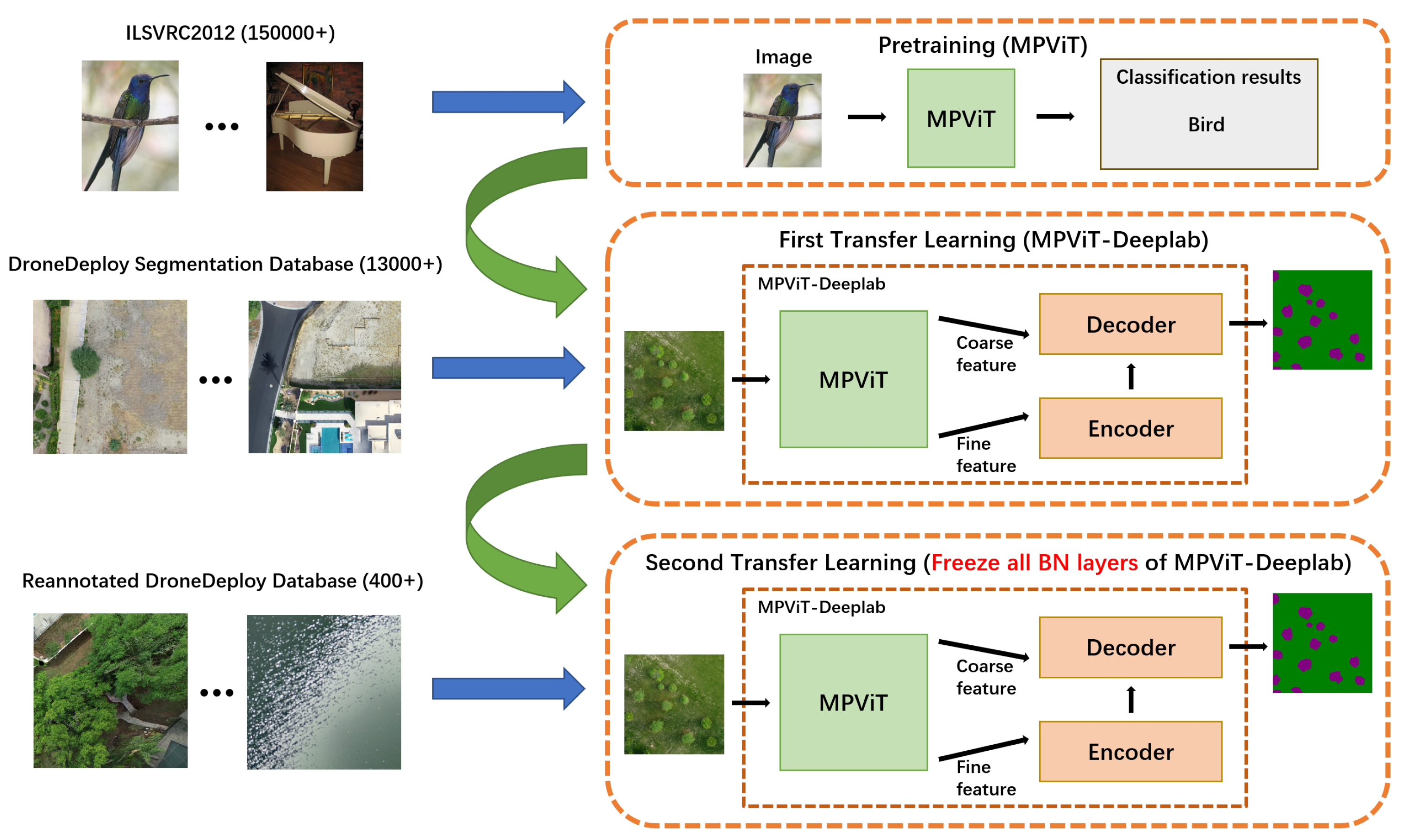
3.2. Three-Stage Transfer Learning

MPViT is a multi-path variant of the ViT model, sharing similar characteristics. One challenge that cannot be avoided is the need for a substantial amount of data and extended training times to achieve the desired segmentation results. Additionally, CSGI extraction datasets pose difficulties in annotation, consume a considerable amount of time, and make it challenging to obtain a large number of labeled samples. In [41], to address the issue of small-sample data, a multi-stage transfer learning approach is employed. Building upon this, we have designed a three-stage transfer learning scheme to tackle training difficulties and data scarcity.

As shown in Figure 6, the three-stage transfer learning method includes three stages: pretraining, the first transfer learning, and the second transfer learning.

Firstly, the pretraining stage is essential. Due to the specificity of MPViT, it needs extensive training with a sufficient amount of data and time to achieve satisfactory results. We conduct prolonged training on the ILSVR2012 dataset and use the obtained weights as initial weights for subsequent transfer learning processes.

Next is the first transfer learning stage. Because of the transition from a classification task to a segmentation task, MPViT is replaced by MPViT-DeepLab in the following two transfer learning processes. In MPViT-DeepLab, the fine and coarse features extracted by MPViT are separately input into the encoder and decoder of DeepLabv3+. In this stage, we input images from the DroneDeploy Segmentation Dataset into MPViT-DeepLab to obtain segmentation results for BUILDING, CLUTTER, VEGETATION, WATER, GROUND, and CAR. This differs significantly from the pretraining classification task. Therefore, in the first transfer learning, we do not freeze any parameters.

Finally, in the second transfer learning stage, the network architecture is similar to the first transfer learning, but we choose to freeze all batch normalization (BN) layers in MPViT-DeepLab. We input the reannotated DroneDeploy Dataset and obtain segmentation results for Grass, Tree, Bush area, Lake, and Terrace greenery. In this task, the segmentation targets partially overlap with the first transfer learning. To fully leverage previous model information, improve segmentation accuracy, reduce the number of parameters and computational burden, and prevent gradient disappearance or explosion, we freeze all batch normalization layers in the MPViT-DeepLab network during the second transfer learning.

3.3. MPViT-DeepLab

CSGI exhibits dense distribution and varying scales, making it challenging to achieve high precision using conventional image segmentation methods. While CNN structures are well-organized and do not rely on extensive data or long training times, they are unable to capture long-range dependencies. On the other hand, ViT exhibits end-to-end dependency but requires a significant amount of data and extensive training time to reach the target accuracy. In light of this, researchers have attempted to combine CNN and Transformer architectures to leverage the strengths of both. Zhang C et al. [42] propose a hybrid network architecture combining CNN and Transformer, using the Swin Transformer as the feature extractor and a U-shaped architecture for the encoder and decoder, for semantic segmentation of ultra-high-resolution remote sensing images. In [43], an MPViT-Unet architecture is used for medical image segmentation. Similarly, in [44], Wang W et al. employ Enhancing Multi-scale Representations With Transformer for the segmentation of remote sensing images, achieving promising results.

DeepLabv3+ has become the preferred segmentation model in many research and application domains due to its outstanding performance and robustness. Azad R et al. introduce TransDeepLab in [45], utilizing the Swin Transformer to extend DeepLabv3 and model the Atrous Spatial Pyramid Pooling (ASPP) module, marking the first use of a purely Transformer-based model to enhance the groundbreaking DeepLab model. Inspired by these works, we utilize MPViT as the backbone feature extraction network, feeding coarse features into the decoder of DeepLabv3+ and fine features into its encoder. This leads to the construction of a hybrid network architecture combining MPViT and DeepLabv3+, named MPViT-DeepLab.

Figure 7 provides an overview of the proposed MPViT-DeepLab network, where DeepLabv3+ serves as the backbone and MPViT functions as the feature extractor. Images first enter the MPViT network. In MPViT, the first Multi-Path Transformer block aggregates features using patches of size $\frac{H}{4}\times \frac{W}{4}$, and the last aggregation uses patches of size $\frac{H}{32}\times \frac{W}{32}$. Therefore, we consider taking the aggregated coarse features after the first aggregation in MPViT as low-level features, which are then fed into the decoder. It first goes through a $1\times 1$ convolution to reduce the channel count, then aggregates with the upsampled result from the encoder, refines the feature with a $3\times 3$ convolution, and finally performs bilinear upsampling to output the segmentation result. Simultaneously, the aggregated fine features are passed into the encoder for atrous convolution.

The atrous convolutions’ function is to enable us to control the resolution of the convolution features and capture multi-scale information. For the input feature $X_i\in {\mathbb{R}}^{H_i\times W_i\times C_i}$, the output feature $Y_i\in {\mathbb{R}}^{H^{\prime }\times W^{\prime }\times C^{\prime }}$ after the atrous convolution has dimensions $H^{\prime }\times W^{\prime }\times C^{\prime }$, where the calculations for $H^{\prime }$ and $W^{\prime }$ are as follows:

$$H^{\prime }=⌊\frac{H_i-k}{r}+1⌋,W^{\prime }=⌊\frac{W_i-k}{r}+1⌋$$

(5)

The calculation formula for the feature $Y_i$ after atrous convolution is as follows:

$$Y_i=\sum _k{X}_{i+r·k}·W_k$$

(6)

In Formula (6), k represents the convolution kernel size, r is the atrous rate, and $W_k$ represents the corresponding weights. For the MPViT network with an output stride of 16, we set the atrous rates for the three intermediate atrous convolutions to [6, 12, 18] to expand the receptive field as much as possible without losing information. We aggregate the features after atrous convolutions, reduce the channel count through a $1\times 1$ convolution, and then upsample the features.

We denote the output of the atrous convolutions in the encoder with atrous rates 6, 12, and 18 as $Y_i$ ($i=1,2,3$), the result of feature pooling as P, the low-level feature input to the decoder as $X_{\mathrm{low}}$, and the feature input to the encoder as X. Combining the $F(·)$ functions, Equation (3) and (6) described in the previous sections, the entire process can be represented as

$$R_{\mathrm{decoder}}=F_{1\times 1}\left(X_{\mathrm{low}}\right),$$

(7)

$$R_{\mathrm{encoder}}=B(F_{1\times 1}\left(\mathrm{Concat}\left([F_{1\times 1}\left(X\right),Y_1,Y_2,Y_3,P]\right)\right),$$

(8)

$$R=B(\mathrm{Concat}\left([R_{\mathrm{decoder}},R_{\mathrm{encoder}}]\right)$$

(9)

In Equations (7)–(9), $B(·)$ represents a bilinear upsampled function by 4, $R_{\mathrm{decoder}}$ represents the features in the decoder after a $1\times 1$ convolution, $R_{\mathrm{encoder}}$ represents the features output by the encoder after upsampling, and $R\in {\mathbb{R}}^{H\times W\times C}$ is the final pixel-wise segmentation result, where C represents the number of classes for segmentation.

4. Results and Discussion

We implement our method based on Pycharm [46] with Python 3.7.0, and all models are trained on a single NVIDIA Quadro RTX 5000 GPU.

We use DeepLabv3+ as the backbone network and MobileNet, ResNet101, Xception, and MPViT as the feature extraction networks (named Mob-D, Res-D, Xce-D, and MPViT-D). In [18], MPViT is categorized into Tiny, Xsmall, Small, and Base based on parameter sizes. In our experiment, we chose the Base version as the feature extractor, with layers set to [1, 3, 8, 3], channels set to [128, 224, 368, 480], and the path of MS-PatchEmbed set to [2, 3, 3, 3]. We set the total number of iterations to 30,000, a learning rate of 0.01, a batch size of 4, and an output stride of 16. For MobileNet, ResNet101, and Xception, the crop size was set to 299, while for MPViT, it was set to 224.

To compare the segmentation performance of several networks, we use the mean intersection over union (MIOU) as the evaluation metric. The specific calculation formula is as follows:

$$MIOU=\frac{TP}{TP+FP+FN},$$

where TP means true positive, FP means false positive, and FN means false negative.

Firstly, we choose DeepLabv3+ as the backbone network and trained Mobilenet, Resnet101, Xception, and MPViT on the DroneDeploy Segmentation Dataset with and without pretraining. We use image chips of sizes $512\times 512$, $300\times 300$, and $224\times 224$ from the DroneDeploy Segmentation Dataset, and find that the $300\times 300$ chip size resulted in the highest training accuracy. Subsequently, for all following experiments, we select remote sensing images with a crop size of $300\times 300$ for training. The training times and MIOU values are shown in

Table 1. Training time (hours) and MIOU (%) of MobileNet, ResNet101, and Xception with DeepLabv3+ and MPViT-DeepLab with and without pretraining on DroneDeploy Segmentation Dataset.

Network	Time (not pre)	MIOU (not pre)	Time (pre)	MIOU (pre)
Mob-D	5	27.0	3.3 (−1.7)	54.0 (+27.0)
Res-D	8.7	28.0	6 (−1.7)	56.9 (+28.9)
Xcep-D	7.5	33.6	2.7 (−4.8)	50.5 (+16.9)
MPViT-D	10.3	30.4	10 (−0.3)	54.7 (+24.3)

:

From Table 1, we can see that the training time for each network varies due to differences in network complexity and the number of parameters. Due to its parallel network structure and a large number of parameters, MPViT-DeepLab obtained the longest training time. In general, pretraining is effective in reducing training time and improving training accuracy. After pretraining, MPViT-DeepLab achieved an MIOU value of 54.7%, which is only 2.2% lower than the highest MIOU achieved by the Resnet101 network and outperforms the other two networks. This indicates that MPViT-DeepLab is suitable for remote sensing image segmentation tasks.

Similarly, using DeepLabv3+ as the backbone network, we then train them on the reannotated DroneDeploy Dataset using their respective pretrained models on ImageNet [38]. We record the intersection over union (IOU) for each combination for the classes Bush area, Grass, Lake, Terrace greenery, and Tree as well as the overall MIOU for CSGI. The specific values are shown in

Table 2. Class segmentation IOU (%) and image segmentation MIOU (%) of MobileNet, ResNet101, and Xception with DeepLabv3+ and MPViT-DeepLab on reannotated DroneDeploy Dataset.

Network	Bush Area	Grass	Lake	Terrace Greenery	Tree	MIOU
Mob-D	75.4	92.9	98.6	67.5	89.0	84.7
Res-D	71.4	93.2	98.4	64.1	89.3	83.3
Xce-D	73.9	92.6	98.3	73.1	87.2	85.0
MPViT-D	71.1	93.8	98.2	74.8	89.4	85.4

.

Analyzing Table 2, MPViT-DeepLab achieves an MIOU of 85.4%, which is 0.4% higher than the Xception and DeepLabV3+ combination. Compared to other combinations, MPViT-DeepLab achieves state-of-the-art results in CSGI extraction. We also observe that MPViT-DeepLab performs well in the segmentation of Green infrastructure categories, such as Grass (+0.6%), Terrace greenery (+1.7%), and Tree (+0.1%). The Terrace greenery segmentation task requires the network to consider the relationship between buildings, greenery, and the environment, and MPViT-DeepLab effectively balances global and local features, resulting in excellent segmentation performance.

To validate the effectiveness of the three-stage transfer learning method and determine which parameters to freeze during the second transfer learning process, we utilize the MPViT-DeepLab parameters trained on the DroneDeploy Segmentation Dataset as the initial weights for training. We conduct comparative experiments under different scenarios, including no freezing (named MPViT-D-T), freezing only the BN layers in MPViT (named MPViT-D-FM), freezing only the BN layers in the DeepLabv3+ (named MPViT-D-FD), and freezing all BN layers in the MPViT-DeepLab (named MPViT-D-FA). The experimental results are presented in

Table 3. Class segmentation IOU (%) and image segmentation MIOU (%) of no freezing, freezing only the BN layers in MPViT, freezing only the BN layers in the DeepLabv3+, and freezing all BN layers in the MPViT-DeepLab on reannotated DroneDeploy Dataset.

Network	Bush Area	Grass	Lake	Terrace Greenery	Tree	MIOU
MPViT-D	71.1	93.8	98.2	74.8	89.4	85.4
MPViT-D-T	73.3	94.3	98.7	66.0	90.8	84.6
MPViT-D-FM	70.5	93.3	98.9	66.8	90.0	83.9
MPViT-D-FD	69.4	93.5	98.7	70.2	89.7	84.3
MPViT-D-FA	72.3	93.4	98.5	73.8	91.5	85.9

.

The first row of Table 3 corresponds to the last row of Table 2 for reference and comparison. Among all the freezing strategies during the second transfer learning process, the MIOU achieved by freezing all BN layers in MPViT-DeepLab is 85.9%, which is 0.5% higher than the MIOU obtained with only the first transfer learning (MPViT-D) and 1.3% higher than the MIOU without freezing any BN layers. Additionally, the strategy of freezing all BN layers in MPViT-DeepLab significantly outperforms the other three freezing methods in the segmentation of Terrace greenery (+2.6%) and Tree (+0.7%), two classes of Green infrastructure. The scenario without freezing any BN layers performs poorly in the segmentation of Terrace greenery, suggesting that, while this approach may have an advantage in simple scenarios due to retaining the original model information, it is not proficient in complex segmentation tasks.

Additionally, we analyze the loss reduction in each scenario in Table 3, as illustrated in Figure 8. According to Figure 8, compared to the approach without the second transfer learning, the gradient of the loss reduction is larger, and the convergence requires fewer epochs, regardless of which layers are frozen. It is evident that adopting the second transfer learning not only improves the accuracy of CSGI extraction but also accelerates the network’s convergence speed.

Some results of CSGI extraction are displayed in Figure 9.

5. Conclusions

In this article, we propose a three-stage transfer learning method to address the challenges of training MPViT and other ViT series networks, which typically require extensive data and time. Additionally, we introduce a hybrid network architecture, MPViT-DeepLab, which exhibits superior integration capabilities for both global and local features compared to traditional neural networks. MPViT-DeepLab achieves state-of-the-art results in the extraction of CSGI.

While MPViT-DeepLab outperforms traditional networks in accuracy, its parallel training structure implies increased computational overhead, and the complexity of the network leads to a higher number of parameters. CSGI extraction holds significant importance in urban planning, and despite the enhanced accuracy of MPViT-DeepLab, future research will focus on simplifying the network to achieve better segmentation results with a more lightweight structure.

References

1. Shen, C.; Li, M.; Li, F.; Chen, J.; Lu, Y. Study on urban green space extraction from QUICKBIRD imagery based on decision tree. In Proceedings of the 2010 18th International Conference on Geoinformatics, Beijing, China, 18–20 June 2010; pp. 1–4. [Google Scholar]
2. Zylshal; Sulma, S.; Yulianto, F.; Nugroho, J.T.; Sofan, P. A support vector machine object based image analysis approach on urban green space extraction using Pleiades-1A imagery. Model. Earth Syst. Environ. 2016, 2, 1–12. [Google Scholar] [CrossRef]
3. Liu, W.; Yue, A.; Shi, W.; Ji, J.; Deng, R. An automatic extraction architecture of urban green space based on DeepLabv3plus semantic segmentation model. In Proceedings of the 2019 IEEE 4th International Conference on Image, Vision and Computing (ICIVC), Xiamen, China, 5–7 July 2019; pp. 311–315. [Google Scholar]
4. Huerta, R.E.; Yépez, F.D.; Lozano-García, D.F.; Guerra Cobian, V.H.; Ferrino Fierro, A.L.; de León Gómez, H.; Cavazos Gonzalez, R.A.; Vargas-Martínez, A. Mapping urban green spaces at the metropolitan level using very high resolution satellite imagery and deep learning techniques for semantic segmentation. Remote Sens. 2021, 13, 2031. [Google Scholar] [CrossRef]
5. Jerome, G. Defining community-scale green infrastructure. In Green Infrastructure; Routledge: London, UK, 2018; pp. 89–95. [Google Scholar]
6. Nie, X.; Duan, M.; Ding, H.; Hu, B.; Wong, E.K. Attention mask R-CNN for ship detection and segmentation from remote sensing images. IEEE Access 2020, 8, 9325–9334. [Google Scholar] [CrossRef]
7. Wang, H.; Chen, X.; Zhang, T.; Xu, Z.; Li, J. CCTNet: Coupled CNN and transformer network for crop segmentation of remote sensing images. Remote Sens. 2022, 14, 1956. [Google Scholar] [CrossRef]
8. Ronneberger, O.; Fischer, P.; Brox, T. U-net: Convolutional networks for biomedical image segmentation. In Proceedings of the Medical Image Computing and Computer-Assisted Intervention—MICCAI 2015: 18th International Conference, Munich, Germany, 5–9 October 2015; pp. 234–241. [Google Scholar]
9. Zhou, Z.; Rahman Siddiquee, M.M.; Tajbakhsh, N.; Liang, J. Unet++: A nested u-net architecture for medical image segmentation. In Proceedings of the Deep Learning in Medical Image Analysis and Multimodal Learning for Clinical Decision Support: 4th International Workshop, DLMIA 2018, and 8th International Workshop, ML-CDS 2018, Held in Conjunction with MICCAI 2018, Granada, Spain, 20 September 2018; pp. 3–11. [Google Scholar]
10. Guo, M.; Liu, H.; Xu, Y.; Huang, Y. Building extraction based on U-Net with an attention block and multiple losses. Remote Sens. 2020, 12, 1400. [Google Scholar] [CrossRef]
11. Chen, Z.; Li, D.; Fan, W.; Guan, H.; Wang, C.; Li, J. Self-attention in reconstruction bias U-Net for semantic segmentation of building rooftops in optical remote sensing images. Remote Sens. 2021, 13, 2524. [Google Scholar] [CrossRef]
12. Chen, L.C.; Papandreou, G.; Kokkinos, I.; Murphy, K.; Yuille, A.L. Semantic image segmentation with deep convolutional nets and fully connected crfs. arXiv 2014, arXiv:1412.7062. [Google Scholar]
13. Chen, L.C.; Papandreou, G.; Kokkinos, I.; Murphy, K.; Yuille, A.L. Deeplab: Semantic image segmentation with deep convolutional nets, atrous convolution, and fully connected crfs. IEEE Trans. Pattern Anal. Mach. Intell. 2017, 40, 834–848. [Google Scholar] [CrossRef]
14. Chen, L.C.; Papandreou, G.; Schroff, F.; Adam, H. Rethinking atrous convolution for semantic image segmentation. arXiv 2017, arXiv:1706.05587. [Google Scholar]
15. Chen, L.C.; Zhu, Y.; Papandreou, G.; Schroff, F.; Adam, H. Encoder-decoder with atrous separable convolution for semantic image segmentation. In Proceedings of the European Conference on Computer Vision (ECCV), Munich, Germany, 8–14 September 2018; pp. 801–818. [Google Scholar]
16. Dosovitskiy, A.; Beyer, L.; Kolesnikov, A.; Weissenborn, D.; Zhai, X.; Unterthiner, T.; Dehghani, M.; Minderer, M.; Heigold, G.; Gelly, S.; et al. An image is worth 16 × 16 words: Transformers for image recognition at scale. arXiv 2020, arXiv:2010.11929. [Google Scholar]
17. Liu, Z.; Lin, Y.; Cao, Y.; Hu, H.; Wei, Y.; Zhang, Z.; Lin, S.; Guo, B. Swin transformer: Hierarchical vision transformer using shifted windows. In Proceedings of the IEEE/CVF International Conference on Computer Vision, Online, 11–17 October 2021; pp. 10012–10022. [Google Scholar]
18. Lee, Y.; Kim, J.; Willette, J.; Hwang, S.J. Mpvit: Multi-path vision transformer for dense prediction. In Proceedings of the IEEE/CVF Conference on Computer Vision and Pattern Recognition, New Orleans, LA, USA, 18–24 June 2022; pp. 7287–7296. [Google Scholar]
19. Samala, R.K.; Chan, H.P.; Hadjiiski, L.M.; Helvie, M.A.; Cha, K.H.; Richter, C.D. Multi-task transfer learning deep convolutional neural network: Application to computer-aided diagnosis of breast cancer on mammograms. Phys. Med. Biol. 2017, 62, 8894. [Google Scholar] [CrossRef] [PubMed]
20. Ghafoorian, M.; Mehrtash, A.; Kapur, T.; Karssemeijer, N.; Marchiori, E.; Pesteie, M.; Guttmann, C.R.; de Leeuw, F.E.; Tempany, C.M.; Van Ginneken, B.; et al. Transfer learning for domain adaptation in MRI: Application in brain lesion segmentation. In Proceedings of the Medical Image Computing and Computer Assisted Intervention—MICCAI 2017: 20th International Conference, Quebec City, QC, Canada, 11–13 September 2017; pp. 516–524. [Google Scholar]
21. Yosinski, J.; Clune, J.; Bengio, Y.; Lipson, H. How transferable are features in deep neural networks? Adv. Neural Inf. Process. Syst. 2014, 27, 3320–3328. [Google Scholar]
22. Raghu, M.; Zhang, C.; Kleinberg, J.; Bengio, S. Transfusion: Understanding transfer learning for medical imaging. Adv. Neural Inf. Process. Syst. 2019, 32, 3342–3352. [Google Scholar]
23. Alzubaidi, L.; Al-Amidie, M.; Al-Asadi, A.; Humaidi, A.J.; Al-Shamma, O.; Fadhel, M.A.; Zhang, J.; Santamaría, J.; Duan, Y. Novel transfer learning approach for medical imaging with limited labeled data. Cancers 2021, 13, 1590. [Google Scholar] [CrossRef] [PubMed]
24. Li, W.; Huang, R.; Li, J.; Liao, Y.; Chen, Z.; He, G.; Yan, R.; Gryllias, K. A perspective survey on deep transfer learning for fault diagnosis in industrial scenarios: Theories, applications and challenges. Mech. Syst. Signal Process. 2022, 167, 108487. [Google Scholar] [CrossRef]
25. Kraus, M.; Feuerriegel, S. Decision support from financial disclosures with deep neural networks and transfer learning. Decis. Support Syst. 2017, 104, 38–48. [Google Scholar] [CrossRef]
26. Jeong, G.; Kim, H.Y. Improving financial trading decisions using deep Q-learning: Predicting the number of shares, action strategies, and transfer learning. Expert Syst. Appl. 2019, 117, 125–138. [Google Scholar] [CrossRef]
27. Mignone, P.; Pio, G.; Ceci, M. Distributed Heterogeneous Transfer Learning for Link Prediction in the Positive Unlabeled Setting. In Proceedings of the 2022 IEEE International Conference on Big Data (Big Data), Osaka, Japan, 17–20 December 2022; pp. 5536–5541. [Google Scholar]
28. Prabhakar, S.K.; Lee, S.W. Holistic approaches to music genre classification using efficient transfer and deep learning techniques. Expert Syst. Appl. 2023, 211, 118636. [Google Scholar] [CrossRef]
29. Chen, B.; Koh, Y.S.; Dobbie, G.; Wu, O.; Coulson, G.; Olivares, G. Online Air Pollution Inference using Concept Recurrence and Transfer Learning. In Proceedings of the 2022 IEEE 9th International Conference on Data Science and Advanced Analytics (DSAA), Shenzhen, China, 13–16 October 2022; pp. 1–10. [Google Scholar]
30. Cao, X.; Wipf, D.; Wen, F.; Duan, G.; Sun, J. A practical transfer learning algorithm for face verification. In Proceedings of the International Conference on Computer Vision, Sydney, Australia, 1–8 December 2013; pp. 3208–3215. [Google Scholar]
31. Gopalakrishnan, K.; Khaitan, S.K.; Choudhary, A.; Agrawal, A. Deep convolutional neural networks with transfer learning for computer vision-based data-driven pavement distress detection. Constr. Build. Mater. 2017, 157, 322–330. [Google Scholar] [CrossRef]
32. Sandler, M.; Howard, A.; Zhu, M.; Zhmoginov, A.; Chen, L.C. Mobilenetv2: Inverted residuals and linear bottlenecks. In Proceedings of the IEEE Conference on Computer Vision and Pattern Recognition, Salt Lake City, UT, USA, 18–23 June 2018; pp. 4510–4520. [Google Scholar]
33. He, K.; Zhang, X.; Ren, S.; Sun, J. Deep residual learning for image recognition. In Proceedings of the IEEE Conference on Computer Vision and Pattern Recognition, Las Vegas, NV, USA, 27–30 June 2016; pp. 770–778. [Google Scholar]
34. Chollet, F. Xception: Deep learning with depthwise separable convolutions. In Proceedings of the IEEE Conference on Computer Vision and Pattern Recognition, Honolulu, HI, USA, 21–26 July 2017; pp. 1251–1258. [Google Scholar]
35. Ioffe, S.; Szegedy, C. Batch normalization: Accelerating deep network training by reducing internal covariate shift. In Proceedings of the International Conference on Machine Learning PMLR, Lille, France, 7–9 July 2015; pp. 448–456. [Google Scholar]
36. Howard, A.; Sandler, M.; Chu, G.; Chen, L.C.; Chen, B.; Tan, M.; Wang, W.; Zhu, Y.; Pang, R.; Vasudevan, V.; et al. Searching for mobilenetv3. In Proceedings of the IEEE/CVF International Conference on Computer Vision, Seoul, Republic of Korea, 27 October–2 November 2019; pp. 1314–1324. [Google Scholar]
37. Xu, W.; Xu, Y.; Chang, T.; Tu, Z. Co-scale conv-attentional image transformers. In Proceedings of the IEEE/CVF International Conference on Computer Vision, Online, 11–17 October 2021; pp. 9981–9990. [Google Scholar]
38. Russakovsky, O.; Deng, J.; Su, H.; Krause, J.; Satheesh, S.; Ma, S.; Huang, Z.; Karpathy, A.; Khosla, A.; Bernstein, M.; et al. ImageNet Large Scale Visual Recognition Challenge. Int. J. Comput. Vis. 2015, 115, 211–252. [Google Scholar] [CrossRef]
39. Dronedeploy. DroneDeploy Segmentation Dataset. Available online: https://github.com/dronedeploy/dd-ml-segmentation-benchmark (accessed on 12 June 2023).
40. Wkentaro. Labelme. Available online: https://github.com/wkentaro/labelme (accessed on 4 July 2023).
41. Zhao, X.; Wang, J. Bridge crack detection based on improved deeplabv3+ and migration learning. J. Comput. Eng. Appl. 2023, 59, 262–269. [Google Scholar]
42. Zhang, C.; Jiang, W.; Zhang, Y.; Wang, W.; Zhao, Q.; Wang, C. Transformer and CNN hybrid deep neural network for semantic segmentation of very-high-resolution remote sensing imagery. IEEE Trans. Geosci. Remote Sens. 2022, 60, 1–20. [Google Scholar] [CrossRef]
43. Hong, Q.; Sun, H.; Li, B.; Peng, A.; Zhou, L.; Zhang, Z. MpVit-Unet: Multi-path Vision Transformer Unet for Sellar Region Lesions Segmentation. In Proceedings of the 2023 5th International Conference on Intelligent Medicine and Image Processing (IMIP), Tianjin, China, 17–20 March 2023; pp. 51–58. [Google Scholar]
44. Wang, W.; Wen, X.; Wang, X.; Tang, C.; Deng, J. CAW: A Remote-Sensing Scene Classification Network Aided by Local Window Attention. Computational Intell. Neurosci. 2022, 2022, 2661231. [Google Scholar] [CrossRef] [PubMed]
45. Azad, R.; Heidari, M.; Shariatnia, M.; Aghdam, E.K.; Karimijafarbigloo, S.; Adeli, E.; Merhof, D. Transdeeplab: Convolution-free transformer-based deeplab v3+ for medical image segmentation. In Proceedings of the International Workshop on PRedictive Intelligence In MEdicine, Singapore, 22 September 2022; pp. 91–102. [Google Scholar]
46. JetBrains. Pycharm. Available online: https://www.jetbrains.com/pycharm/ (accessed on 6 April 2023).
Figure 1. An overview of MPViT network structure for image classification.
Information 15 00015 g001
Figure 2. Specific architecture of the Multi-Scale PatchEmbed block in MPViT.
Information 15 00015 g002
Figure 3. Specific architecture of the multi-path Transformer block in MPViT.
Information 15 00015 g003
Figure 4. Specific network architecture of encoder and decoder of DeepLabv3+.
Information 15 00015 g004
Figure 5. A few samples of reannotated DroneDeploy Dataset, where class labels corresponding to colors are shown on the right.
Information 15 00015 g005
Figure 6. An overview of the three-stage MPViT-DeepLab transfer learning, which includes three stages: pretraining, the first transfer learning, and the second transfer learning.
Information 15 00015 g006
Figure 7. An overview of MPViT-DeepLab hybrid network architecture.
Information 15 00015 g007
Figure 8. Loss reduction of MPViT-DeepLab networks with and without transfer learning.
Information 15 00015 g008
Figure 9. Some CSGI extraction results of networks in Table 2 and Table 3.
Information 15 00015 g009