Article

Detecting Abnormal Behaviors in Dementia Patients Using Lifelog Data: A Machine Learning Approach

1
Department of Computer Engineering, Sejong University, Seoul 05006, Republic of Korea
2
Department of Convergence Engineering for Intelligent Drones, Sejong University, Seoul 05006, Republic of Korea
*
Author to whom correspondence should be addressed.
Information 2023, 14(8), 433; https://doi.org/10.3390/info14080433
Submission received: 17 July 2023 / Revised: 30 July 2023 / Accepted: 31 July 2023 / Published: 1 August 2023
(This article belongs to the Special Issue IoT-Based Systems for Safe and Secure Smart Cities)

Abstract

:
In this paper, a proof-of-concept method for detecting abnormal behavior in dementia patients based on a single case study is proposed. This method incorporates the collection of lifelog data using affordable sensors and the development of a machine-learning-based system. Such an approach has the potential to enable the prompt detection of abnormal behavior in dementia patients within nursing homes and to send alerts to caregivers, which could potentially reduce their workload and decrease the risk of accidents and injuries. In a proof-of-concept experiment conducted on a single dementia patient in a Korean nursing home, the proposed system, specifically the multilayer perceptron model, demonstrated exceptional performance, achieving an accuracy of 0.99, a precision of 1.00, a recall of 1.00, and an F1 score of 1.00. While being cost-effective and adaptable to various nursing homes, these results should be interpreted as preliminary, being based on a limited sample. Future research is aimed at validating and improving the performance of the abnormal behavior detection system by expanding the experiments to include lifelog data from multiple nursing homes and a larger cohort of dementia patients. The potential application of this system extends beyond healthcare and medical fields, reaching into smart home environments and various other facilities. This study underscores the potential of this system to enhance patient safety, alleviate family concerns, and reduce societal costs, thereby contributing to the improvement of the quality of life for dementia patients.

1. Introduction

The term “dementia”, also known as “major neurocognitive disorder”, is not a reference to a specific disease but to a series of symptoms caused by various diseases. Common underlying conditions, such as Alzheimer’s disease, stroke, and Parkinson’s disease, typically give rise to dementia symptoms. These symptoms are prevalent in the population aged 65 and older [1], with notable features including the presence of beta-amyloid and tau proteins in the brain, which accumulate to the extent that they interfere with normal cognitive function. This phenomenon manifests as changes in memory, abstract thinking, judgment, behavior, mood, and emotions, as well as disruptions in physical control [2].
Globally, one person is diagnosed with dementia every three seconds. As of 2020, over 50 million people worldwide live with dementia, a number expected to nearly double every 20 years, reaching 78 million by 2030 and 139 million by 2050. The annual total cost of dementia worldwide exceeds $1.3 trillion, with this figure projected to increase to $2.8 trillion by 2030 [3].
Dementia is one of the most cost-intensive diseases in society, accounting for 85% of the costs associated with family or community care [3,4] and contributing significantly to disability and nursing home placement [5]. To reduce expenditure, efforts can be initiated by reducing the workload of caregivers. Various care services are performed by caregivers, such as physical activity support, emotional support, cognitive activity support, dementia management support services, and emergency services. Among these, dementia management support services, which involve dealing with abnormal behaviors in dementia patients, pose the most significant challenge. If abnormal behaviors in dementia patients lead to accidents, injuries or even death can result. Therefore, immediate protection must be provided by caregivers when such behaviors occur. However, in most rehabilitation nursing homes currently caring for dementia patients, the system relies on caregivers periodically patrolling and responding to abnormal behavior. Consequently, providing immediate protection for dementia patients under these circumstances is challenging.
To address this issue, the optimal solution would be to collect images or videos of abnormal behavior in dementia patients and train machine learning algorithms on this data. However, building such a system in most rehabilitation nursing homes is challenging due to the significant financial burden it entails.
Therefore, in this paper, a system is proposed that uses affordable sensors to collect lifelog data and train machine learning algorithms to detect abnormal behavior in dementia patients and immediately alert caregivers. Lifelog data is collected by attaching sensors to various pieces of furniture within nursing homes and having dementia patients wear smartwatches. When patients approach furniture within the nursing home, lifelog data is transmitted to the lifelog sensor hub.
The organization of the paper is as follows: In Section 2, research cases on abnormal behavior detection are discussed, the machine learning models utilized in this paper are examined, and previous studies are reviewed. Section 3 is dedicated to the introduction of the system design and the data employed in the experiments. The experimental results obtained by using the system and data introduced in Section 3 are presented in Section 4. Lastly, the study is concluded in Section 5.

2. Related Works

Research on abnormal behavior detection is actively and continuously being conducted. Methods for detecting abnormal behavior encompass behavioral observation, interviews, standardized assessment tools, biometric signal measurement, and image recognition technology. This section delves into studies that employ machine learning techniques for abnormal behavior detection and introduces the machine learning algorithm models utilized in this research.

2.1. Research on Detection of Abnormal Behavior Based on Machine Learning

Abnormal human behavior in both densely and sparsely populated environments was detected by Kuppusamy, P. et al. [6]. The video clip datasets used were the UCF-Crime Dataset [7] and the UCSD Anomaly Detection Dataset [8]. These datasets were used to train CNN (Convolutional Neural Networks) [9]. The result demonstrated an accuracy of 98.5% in densely populated environments and 99.5% in less densely populated environments.
Niu, Z. et al. [10] suggested an abnormal detection approach based on the Ensemble Active Semi-Supervised Learning (ADESSA) method, which amalgamates the benefits of semi-supervised learning and active learning. The detection accuracy was enhanced, and false alarms were reduced by employing a combination of multiple classifiers in the proposed approach. The ADESSA model was trained on the NSL-KDD Dataset [11] and the KDD Cup 99 Dataset [12], attaining an accuracy of 99.2%.
Wang, J. et al. [13] introduced a deep-learning-based approach that utilizes video data for detecting abnormal human behavior. Data were generated by recording videos of abnormal human behavior, and a deep learning model was trained on these data. CNN was used to extract features from video frames, which were then input into long short-term memory (LSTM) [14] for classification, yielding an accuracy of 92.5% in detecting abnormal human behavior.
Han R. et al. [15] put forth an abnormal behavior detection method aimed at detecting malicious activities based on host behavior data. Host behavior data were collected in a time series format by configuring a testbed. To tackle the imbalance of the collected data, adaptive synthetic (ADASYN) [16] and synthetic minority over-sampling techniques (SMOTE) [17] were employed, and models such as K-Nearest Neighbor (KNN) [18], Naïve Bayes (NB) [19], Random Forest (RF) [20], Autoencoder (AE) [21], and Memory-Augmented Deep Autoencoder (MemAE) [22] were trained. The SMOTE-based MemAE model achieved an F1 score of 1.00 and an area under the receiver operating characteristic curve (AUROC) of 0.98.
Huang, C. et al. [23] proposed a temporal-aware contrastive network (TAC-Net), which is a deep-contrastive-learning-based abnormal event detection framework. On datasets such as UCSD [24], CUHK Avenue [25], and ShanghaiTech [26], models like MemAE [22], ISTL [27], sRNN-AE [28], and TAC-Net [23] were trained and tested. The suggested TAC-Net achieved the highest accuracy of 98.1%.
Chen, G. et al. [29] introduced a neuromorphic vision-based abnormal event detection system. The public NeuroAED dataset [29] was created, consisting of four sub-datasets (walking, campus, square, and staircase datasets). Additionally, the Event-based Multiscale Spatial-Temporal (EMST) model [29] was proposed for experimentation. Models such as EMST, Sparse Representation (SR) [30], and K-Singular Value Decomposition (K-SVD) [31] were trained on the dataset, ultimately achieving an accuracy of 95.8%.
Li, G. et al. [32] examined papers that conducted anomaly detection on multivariate time series data using machine learning algorithms. Based on their findings, it was determined that most studies predominantly employed LSTM [14] and AE [21] models, achieving high accuracy with these models.
Various approaches for detecting abnormal behavior were considered in the studies. Research that focused on detecting abnormal behavior based on video data primarily utilized CNN models. In other studies, a diverse range of models were employed, and as demonstrated in Table 1, models such as KNN, NB, and RF were used when detecting abnormal behavior with time series data.

2.2. Machine Learning Argorithms

In this study, a dementia patient abnormal behavior detection system based on lifelog data will be developed by applying not only models like KNN and RF, as examined in Section 2.1, but also additional models, such as logistic regression (LR) [33], decision tree (DT) [34], support vector machines (SVM) [35], and multi-layer perceptron (MLP) [36]. By comparing and analyzing the results obtained in the research, the optimal model can be selected, and tangible outcomes that contribute to the health and safety of dementia patients are expected.
The data introduced in Section 3, to be presented later, possess a very simple structure. Applying complex models like AE, MemAE, and LSTM to such data may cause overfitting and result in lower accuracy. Therefore, this study will exclude the use of AE, MemAE, and LSTM, focusing on other models instead.
In this section, the principles, advantages, and disadvantages of the models to be used in the experiments are briefly described. This will aid readers in understanding how each model is applied to the data and contributes to the detection of abnormal behavior.

2.2.1. K-Nearest Neighbors (KNN)

KNN is a simple supervised learning algorithm that can be used for both classification and regression problems.
  • Principle: KNN classifies a data point based on the majority class of its k-nearest neighbors in the feature space.
  • Pros: Easy to implement, works well with small datasets, and requires no training.
  • Cons: Computationally expensive for large datasets, sensitive to noise and irrelevant features, and performance decreases as the dimensionality of the feature space increases.

2.2.2. Random Forest (RF)

RF is an ensemble learning method that constructs multiple decision trees to improve overall prediction accuracy.
  • Principle: Combines the predictions of multiple decision trees, which are trained on different subsets of the dataset, to make a final decision.
  • Pros: Reduces overfitting, handles missing values well, and provides good feature importance estimates.
  • Cons: Can be slow to train and predict, particularly with many trees, and may struggle with very high-dimensional datasets.

2.2.3. Logistic Regression (LR)

LR is a statistical method for binary classification problems.
  • Principle: Models the probability of the outcome using the logistic function applied to a linear combination of input features.
  • Pros: Easy to implement, fast to train, and provides interpretable feature coefficients.
  • Cons: Assumes a linear relationship between features and the log-odds of the outcome and may struggle with complex decision boundaries.

2.2.4. Decision Tree (DT)

DT is a type of model used for both classification and regression tasks.
  • Principle: Splits the data into subsets based on feature values, recursively constructing a tree-like structure with decision nodes and leaf nodes.
  • Pros: Easy to understand and interpret, can handle both numerical and categorical data, and requires little preprocessing.
  • Cons (Continued): Prone to overfitting, sensitive to small changes in the data, and may produce biased trees if some classes dominate.

2.2.5. Support Vector Machines (SVM)

SVM is a supervised learning algorithm for classification and regression tasks.
  • Principle: Finds the optimal hyperplane that maximizes the margin between different classes in the feature space.
  • Pros: Effective in high-dimensional spaces, versatile due to the use of kernel functions, and provides good generalization performance.
  • Cons: Can be slow to train for large datasets, requires parameter tuning, and may struggle with noisy or overlapping classes.

2.2.6. Multi-Layer Perceptron (MLP)

An MLP is a type of feedforward artificial neural network, typically used for supervised learning tasks such as classification and regression.
  • Principle: Consists of an input layer, one or more hidden layers, and an output layer, with each layer containing a set of interconnected nodes (neurons). The network is trained using backpropagation and gradient descent.
  • Pros: Can learn complex non-linear relationships between input and output and can be used for a wide range of applications.
  • Cons: Can be sensitive to hyperparameter choices, prone to overfitting, and may require significant computational resources for large networks.

3. Design and Implementation of Machine-Learning-Based Dementia Patient Abnormal Behavior Detection System

In this section, the design and implementation of a machine-learning-based system for detecting abnormal behavior in dementia patients are described. The proposed system employs various machine learning models, such as those outlined in Section 2.2, to detect and classify the behavior of dementia patients. Furthermore, an overview of the data collection methods and descriptions for the dementia patients’ lifelog data are provided.

3.1. System Structure and Description

This proof-of-concept study was conducted in an actual nursing home in South Korea. The experiment took place on one floor dedicated to caring for dementia patients within the nursing home, and the data of one dementia patient were utilized for the experiment. As illustrated in Figure 1, the system is a machine learning-based system for detecting abnormal behavior in dementia patients, and it collects lifelogs (smartwatch ID, sensor ID, time) from lifelog sensors attached to furniture within the nursing home.
When a dementia patient wearing a smartwatch interacts with the lifelog sensors, such as through shaking, the corresponding lifelog (smartwatch ID, sensor ID, time) is transmitted to the lifelog sensor hub and data collection occurs. The lifelog is then stored in the database within the lifelog data management server on the Amazon Web Services (AWS) cloud. At one-minute intervals, the lifelog is sent to the abnormal behavior detection server, where the model determining the presence of abnormal behavior is executed. The resulting decision is subsequently transmitted to the smartphones of doctors and nurses via an app.
The smartphone app, designed as an experimental application to run on Android devices, is exclusively installed on the smartphones of participating doctors and nurses. This app generates audible and vibratory alarms whenever abnormal behaviors occur in dementia patients, allowing users to verify the timing of these incidents, as illustrated in Figure 1 of the smartphone application interface.
It is important to acknowledge the limitation of this study, which is that it includes data from a single dementia patient in a single environment. While this allows for a more controlled examination of the feasibility of the system, it may limit the generalizability of the results. Future work should aim to include data from multiple patients in various settings, including those without dementia, to evaluate the robustness of the proposed system more thoroughly. We see this work as an initial step towards a more comprehensive investigation into machine-learning-based abnormal behavior detection in dementia patients.

3.2. Lifelog Sensor Device

The lifelog sensor device is utilized to detect the activities of dementia patients by being attached to furniture within the nursing home. These sensors consist of adhesive lifelog sensors, smartwatches, and lifelog sensor hubs. To minimize implementation costs, these sensor devices are equipped with a minimal set of internal sensors and batteries.
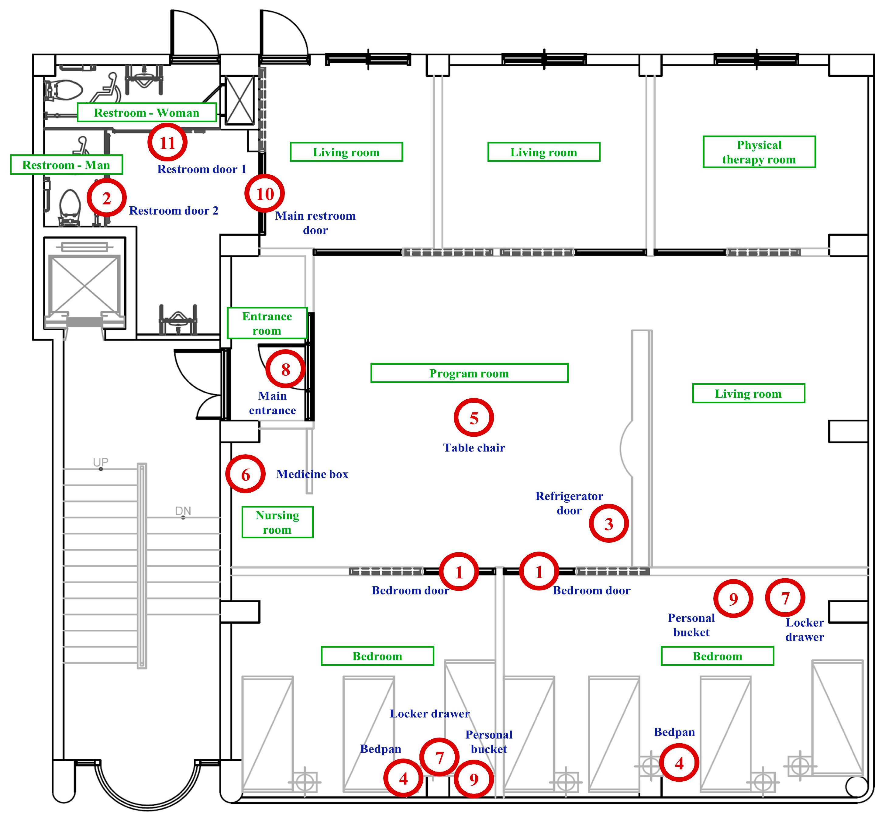
The locations where adhesive lifelog sensors are attached are shown in Figure 2, and the sensor numbers, locations, furniture, and equipment are listed in Table 2. Actual photos of the furniture within the nursing home with attached sensors are displayed in Figure 3.
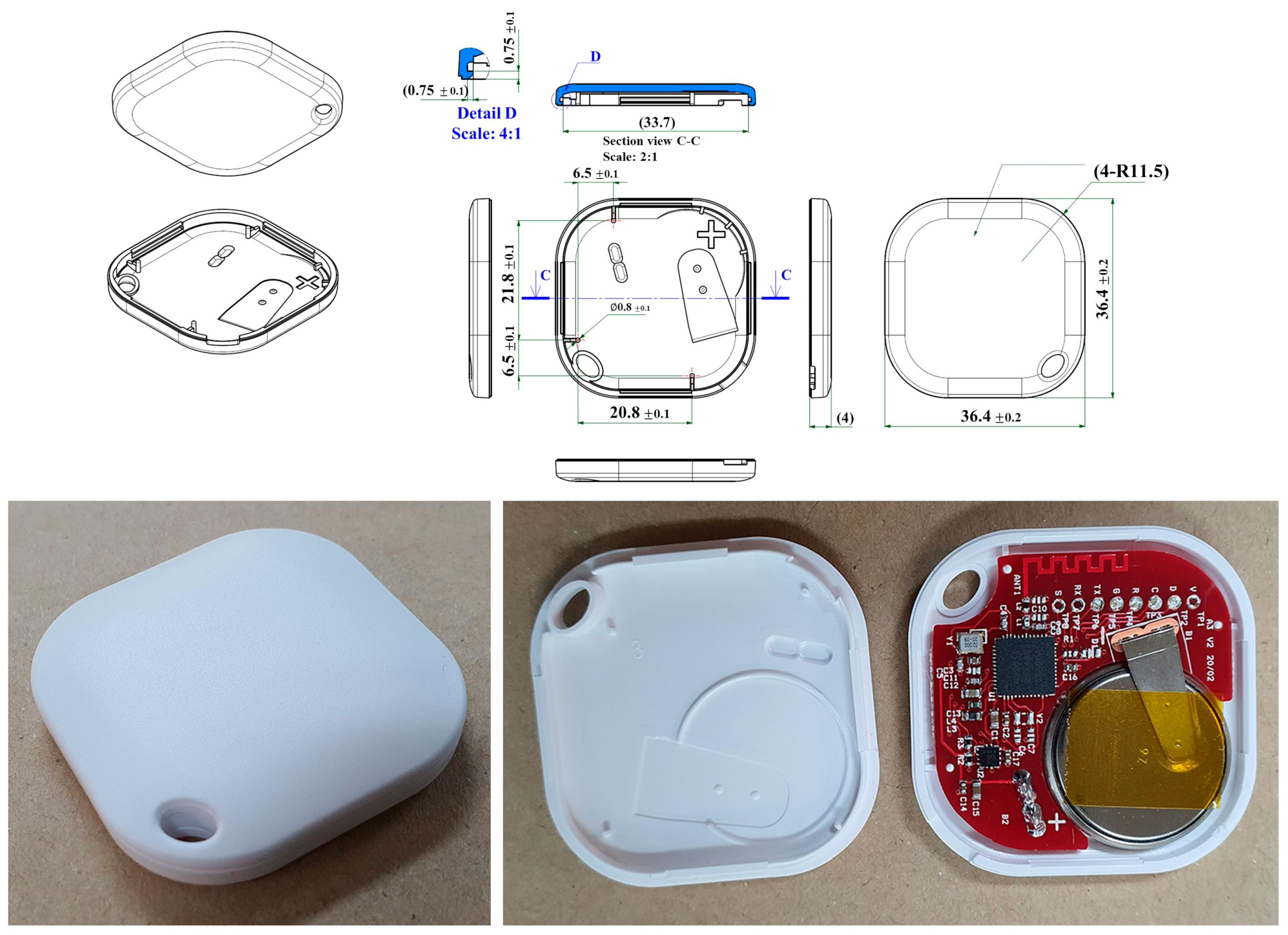
The adhesive lifelog sensor features a square outer panel made of acrylonitrile–butadiene–styrene [37], and its interior is composed of a motion-detecting sensor and battery, as depicted in Figure 4.
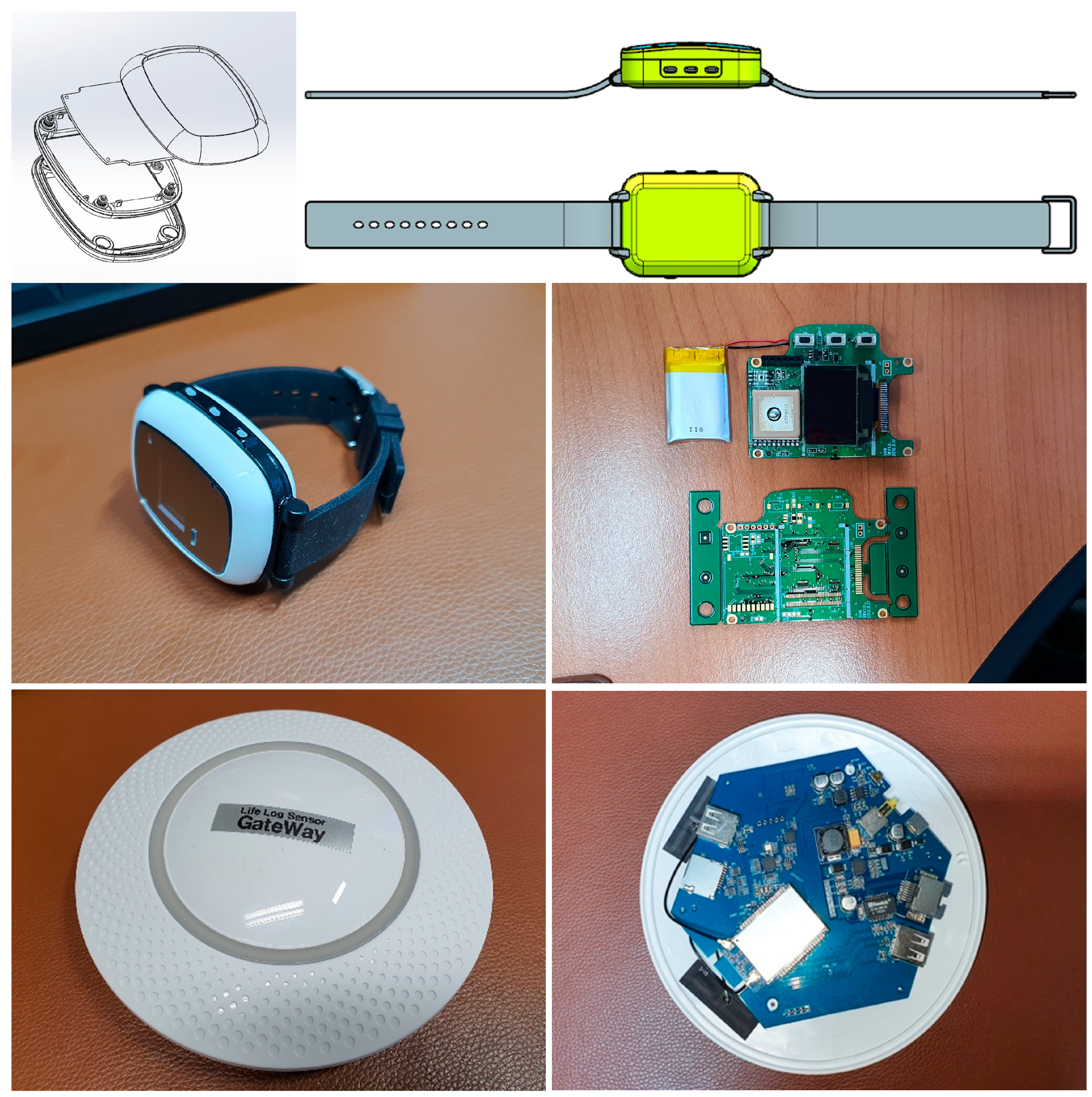
The smartwatch, worn by dementia patients, can be charged using a micro-USB charger and detects the movements of the paired lifelog sensors via Bluetooth without any special settings according to the registered device ID on the server. The smartwatch has an outer panel made of polycarbonate and contains a battery, Bluetooth module, and display module internally. Only dementia patients participating in the experiment wear such smartwatches. The lifelog sensor hub serves to receive the lifelog data transmitted by the smartwatch and forwards it to the server. Therefore, it is simply composed of a Bluetooth transceiver module and a battery. The smartwatch and lifelog sensor hub are configured as shown in Figure 5.

3.3. Lifelog Dataset

Dementia patients may exhibit abnormal behaviors when they are confused in situations that are difficult to understand, feel anxious, or experience loneliness. Representative examples include insomnia, confusingly wearing clothes or bed sheets, and problematic behavior in the restroom, which are summarized in Table 3.
Lifelog sensors play a role in detecting and analyzing the data collected from dementia patients’ abnormal behaviors to determine whether these behaviors are abnormal. For this purpose, the lifelog sensors are equipped with the capability to detect abnormal behaviors, such as repetitive actions in daily life and sleep disturbances. Thus, the lifelog sensors can detect abnormal behaviors like the repetitive behaviors and sleep disturbances introduced in Table 3. Accurately detecting and analyzing these abnormal behaviors is important for understanding and managing the health status of dementia patients.
A part of the lifelog dataset collected using the devices introduced in Section 3.2 is presented in Table 4. This dataset consists of date, time, sensor number, and labels, where the sensor number corresponds to the numbers described in Figure 2 and Table 2. The labels include three labels: 0 for normal behavior, 1 for repetitive behaviors, and 2 for sleep disturbances, which were manually assigned by the caregivers attending to the dementia patients.
The sensor data was collected from a single dementia patient who had given consent for their personal information to be used. The collection period was from 11 November 2022 to 20 December 2020, and during this time, a total of 65,844 rows of data were collected. There were only a small number of missing data entries, most of which were due to temporary sensor malfunctions or communication issues. Whenever sensor malfunctions were identified, the affected sensors were promptly replaced.

4. Experiment and Experimental Results

In this section, the lifelog dataset introduced in Table 4 is preprocessed, the parameters of the learning models are explained, and the performance results of the models are presented.

4.1. Data Preprocessing

After preprocessing the lifelog dataset introduced in Table 4, the learning models were set up and experiments were conducted. The data preprocessing involved the following steps: First, the date and time were converted to datetime format and the datetime column was set as the index. Upon examining the data in Table 4, missing values were found where the sensors did not function. Consequently, all data rows with missing values were removed. Next, appropriate features were added: total_activations (TA) represent the total number of activated neurons in the entire lifelog dataset, max_activation (MaxA) indicates the highest number of activated neurons in each lifelog, mean_activation (MeanA) denotes the average number of activated neurons in each lifelog, and std_activation (SA) signifies the standard deviation of the number of sensor activations. Finally, the preprocessed data was divided into training and testing sets in a 7:3 ratio. The preprocessed data is shown in Table 5.
Visualization is essential for comparing data before and after preprocessing. Dimensionality reduction techniques, such as T-distributed stochastic neighbor embedding (t-SNE) [38] and uniform manifold approximation and projection (UMAP) [39], are commonly used for this purpose. Dimensionality reduction is a technique in which high-dimensional data is simplified into lower dimensions for easier visualization and analysis. T-SNE is a nonlinear dimensionality reduction technique that maps high-dimensional data to lower dimensions while preserving similarities. However, t-SNE can have slow computational speeds and performance issues. UMAP was developed to address these problems. This nonlinear dimensionality reduction technique is like t-SNE but operates faster and can be applied to large-scale data. UMAP aims to preserve the similarity between high-dimensional data points in lower dimensions. It achieves this by selecting an optimized approximation method depending on the complexity of the data. Consequently, UMAP is better suited for the visualization and analysis of large-scale and high-dimensional data.
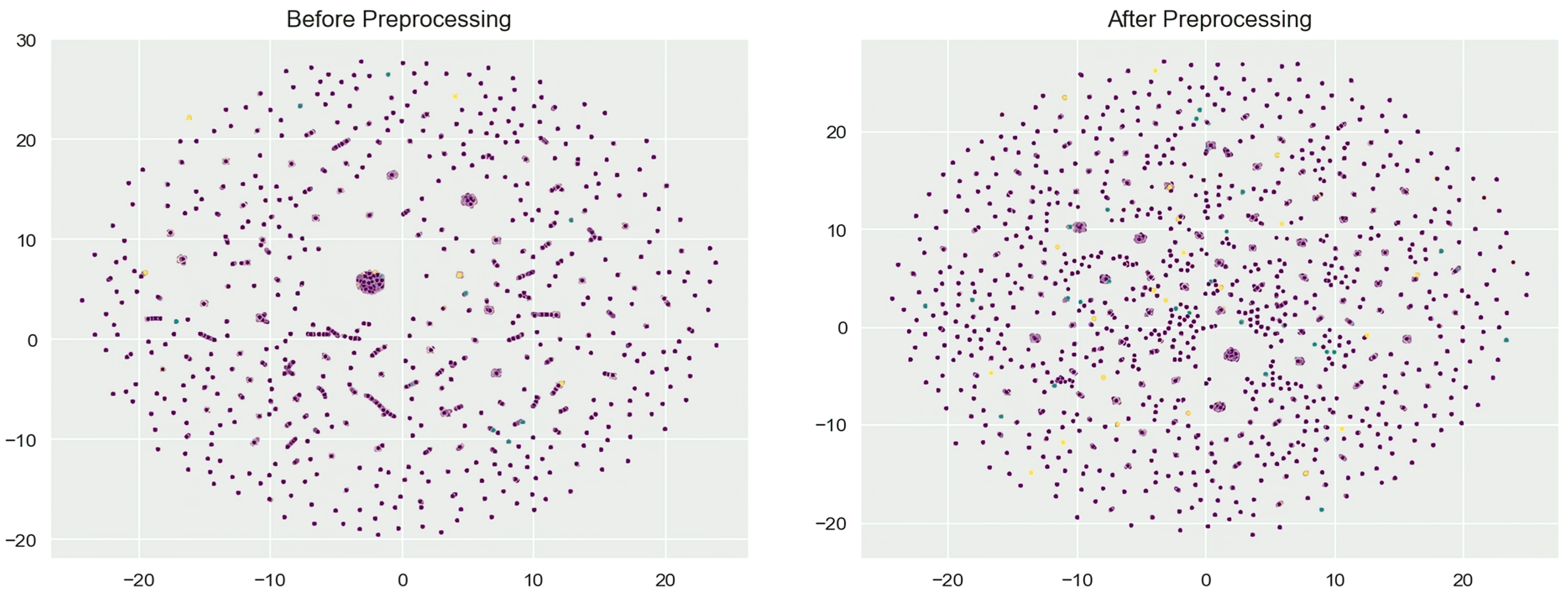
In this study, UMAP was utilized to visualize the data both before and after preprocessing, as depicted in Figure 6. The color assignments for the dots are as follows: purple dots represent label 0, green dots signify label 1, and yellow dots denote label 2. Prior to preprocessing, data points indicating normal behaviors, repetitive behaviors, and sleep disturbances were closely clustered together. This dense clustering made distinguishing between different behavioral patterns challenging due to their overlap.
However, after preprocessing, the data distribution became more explicit, with the different behavior data points becoming more dispersed. It’s important to note here that we intentionally aimed for a sparse feature map. This may seem counterintuitive since compact and well-separated clusters typically improve classification. However, in our context, in which we deal with various behaviors that might interact and overlap, a sparse feature map brings a particular advantage.
Specifically, this sparsity in the feature map reveals a nuanced view of the underlying data structure. It helps in uncovering subtler patterns and potential outliers that might be missed in a more densely clustered feature map. Furthermore, the sparse feature map offers additional insights into the relations and distances between different clusters. These insights are particularly valuable in our study as they enhance our understanding of the behavior patterns of dementia patients. We believe this approach, although somewhat unconventional, provides a more comprehensive overview of the behavioral patterns we are studying.

4.2. Parameters and Performance Evaluation of Models

In the experiment, a total of six models were used: KNN, RF, LR, DT, SVM, and MLP, as introduced in Section 2.2. The initial parameters for these models were set as shown in Table 6 based on default settings typically used in machine learning libraries, such as Scikit-learn, and guided by previous empirical studies.
Recognizing that the model performance can be highly dependent on the chosen parameters, we embarked on a fine-tuning process. We utilized techniques like grid search and cross-validation to ensure the parameters’ suitability for our specific dataset. The parameters were adjusted iteratively based on the models’ performance in preliminary runs.
Table 6 hence represents the best-performing parameter settings from our experimental runs. It is crucial to highlight that these parameters are tailored to our specific dataset and may not be optimal for other datasets or problem contexts. Therefore, when applying these models to other datasets or problem contexts, a similar process of parameter tuning should be performed.
In this study, confusion matrices were used, and accuracy, precision, recall, and F1 score were calculated to evaluate the performance of each model. Localization curve (LC), receiver operating characteristic (ROC), and precision–recall curve (PRC) were also utilized. First, the confusion matrix is a visualization tool that helps measure the performance of classifiers, providing an intuitive view of the relationship between actual and predicted labels. Prediction results are classified as true positive (TP), true negative (TN), false positive (FP), and false negative (FN) when compared to the actual class. Table 7 is an example of a confusion matrix for a binary classification model with two classes (positive/negative). In Table 7, TP refers to cases correctly predicted as positive when they are positive, and TN refers to cases correctly predicted as negative when they are negative. FP refers to cases incorrectly predicted as positive when they are negative, and FN refers to cases incorrectly predicted as negative when they are positive.
To evaluate the performance of the models, metrics such as accuracy, precision, recall, and F1 score were used. These metrics are described as follows:
  • Accuracy: This metric represents the proportion of instances in which the model’s predictions match the actual values. In other words, it signifies the ratio of samples that the model correctly predicted out of the total samples. Accuracy is one of the fundamental indicators for evaluating the performance of a classification model and is a representative metric that demonstrates how accurately the model predicts. Accuracy is calculated as shown in Equation (1).
    Accuracy = TP + TN TP + TN + FP + FN
  • Precision: This metric represents the proportion of samples that are positive among the results predicted as positive by the model. In other words, it indicates how many of the samples predicted as positive by the model are genuinely positive. A high precision means that most samples predicted as positive by the model are positive. Precision is calculated as shown in Equation (2).
    Precision = TP TP + FP
  • Recall: This metric represents the proportion of samples predicted as positive by the model among the actual positive samples. In other words, it indicates how many of the actual positive samples the model predicts as positive. A high recall means that the model accurately identifies most of the positive samples. Recall is calculated as shown in Equation (3).
    Recall = TP TP + FN
  • F1 Score: This metric is the harmonic mean of precision and recall. It represents the average value considering both precision and recall, indicating the overall performance of the model. A high F1 score implies that both precision and recall are high. F1 score reaches its highest value when precision and recall are balanced. F1 score is calculated as shown in Equation (4).
    F 1 - Score = 2 Precision Recall Precision + Recall
Ultimately, to evaluate the performance of the models, metrics such as accuracy, precision, recall, and F1 score were calculated, as shown in Table 8. The logistic regression model exhibited high precision, recall, and F1 score for labels 0 and 2 but low performance for label 1. The decision tree model displayed high precision, recall, and F1 score for all labels. The random forest model demonstrated high precision, recall, and F1 score for labels 0 and 2 but low recall for label 1. The SVM model showed high performance for label 0 but low performance for labels 1 and 2. The KNN model revealed high precision, recall, and F1 score for labels 0 and 2 but low performance for label 1. The MLP model presented high precision, recall, and F1 score for all labels, offering the highest performance among all models.
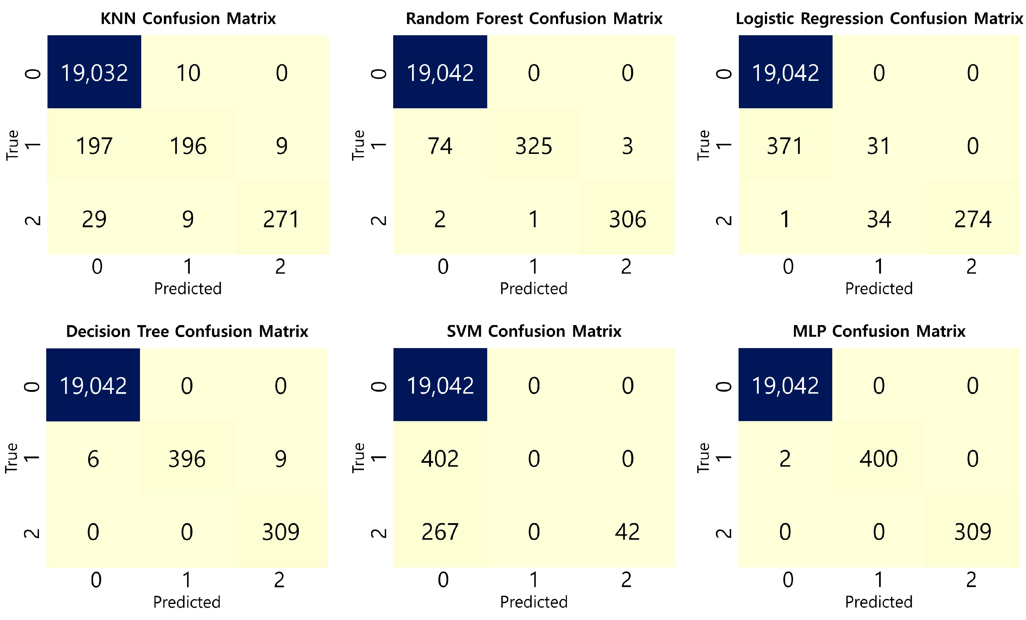
In this study, the confusion matrix for each model was visualized, allowing for a more detailed analysis of the model’s prediction results by examining the TP, TN, FP, and FN values. To create a confusion matrix for each model, the model was first fitted to the training dataset and predictions were made on the test dataset. Subsequently, the confusion matrix was visualized using the plot_confusion_matrix function. This function employed the heatmap feature from the Seaborn library to represent the confusion matrix as a color-coded grid. Each cell displayed the number of actual labels and predicted labels for the corresponding labels. The generated confusion matrices enabled a comparative analysis of the performance of each model. By examining Figure 7, it can be observed that all models made correct predictions, with the KNN model having the lowest prediction label count at 19,032, but the performance difference was minimal due to a difference of approximately 10 from the other models.
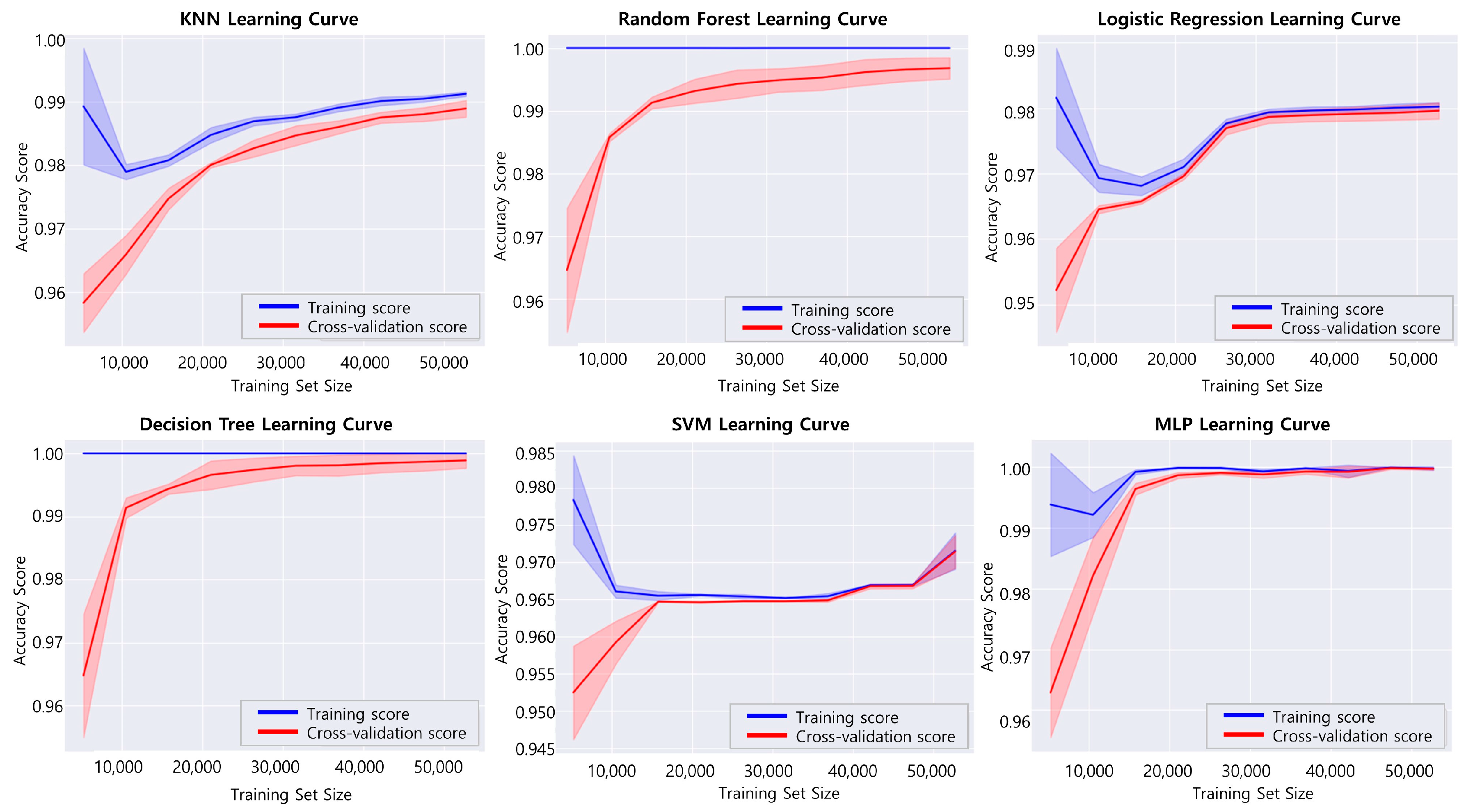
Secondly, LCs were found to be useful visualization tools for evaluating the accuracy of each label when classifiers make predictions. LCs display how the accuracy for a specific label varies within a certain range, which can help identify the range in which predictions are incorrect for that label. LCs are commonly used for assessing the reliability and error analysis of classification models and can be generalized for other classification problems. To generate an LC, the classification threshold for each label was adjusted based on the predicted probabilities. Next, samples of each label were selected from the test dataset, and the accuracy of the selected samples was calculated while adjusting the classification threshold. This process was repeated with the threshold varying from 0 to 1, generating the LC. The resulting LC visualized the accuracy and classification threshold changes for the given label, allowing for comparative analysis of model performance. By examining Figure 8, it can be confirmed that the RF, DT, and MLP curves show the best accuracy, trending upward.
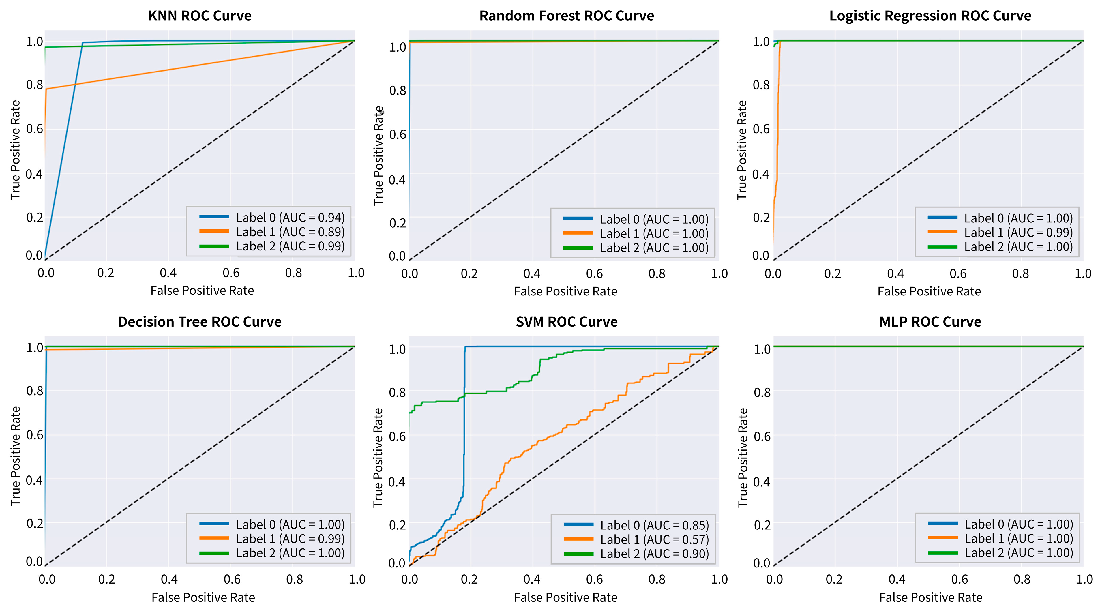
Thirdly, receiver operating characteristic curves are a visualization tool used to evaluate the performance of binary classification models. These curves plot the TPR against the FPR for different classification thresholds. The TPR represents the proportion of actual positives that are correctly identified, while FPR represents the proportion of actual negatives that are incorrectly identified as positive. The area under the curve (AUC) of the ROC curve is a widely used metric for measuring the performance of classification models, with a value closer to 1 indicating better performance. ROC curves provide a way to visually compare the performance of different models. In Figure 9, we can observe that the RF, DT, LR, and MLP models exhibit high performance, with RF and MLP achieving the best performance, with an AUC of 1.00 for all labels (0, 1, 2).
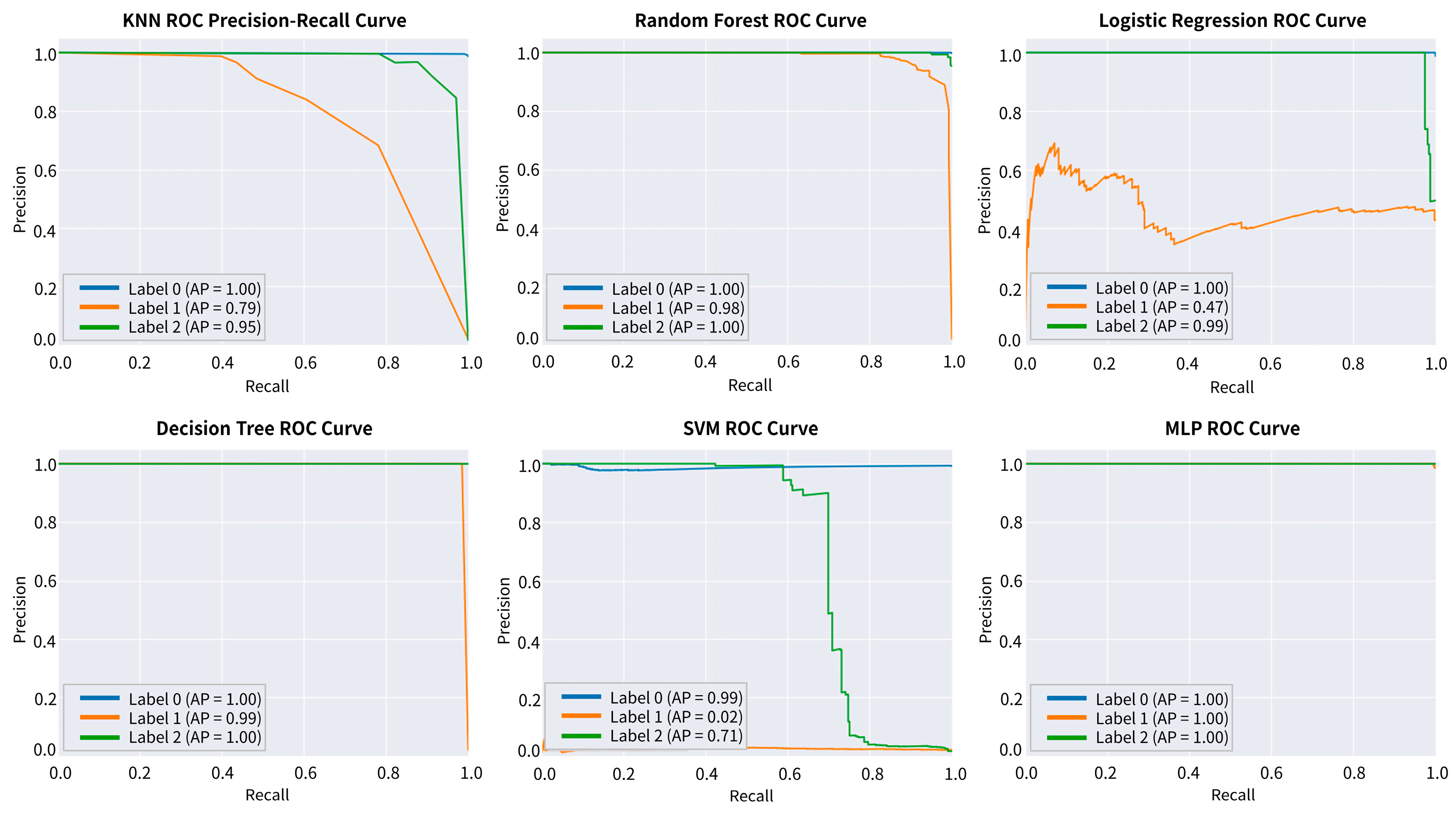
In this study, precision–recall curve is used to evaluate the performance of binary classifiers. PRC is like ROC curves but is more suitable for imbalanced class datasets since it considers classification errors between classes and visualizes the relationship between precision and recall. PRCs display the changes in precision and recall at various thresholds, using a curve with recall on the X-axis and precision on the Y-axis as an indicator to evaluate the performance of classification models. Precision represents the proportion of true positive samples among the positive samples predicted by the model, while recall represents the proportion of true positive samples among the actual positive samples. Average precision (AP) is the average of precision values across all recall values and represents the average of precision values rather than the area under the PRC graph. The higher the AP, the better the model’s performance. PRCs are particularly useful when evaluating the performance of classification models for imbalanced class datasets. After analyzing the PRCs for each model, it was found that RF, DT, and MLP exhibit high performance, with MLP achieving the best performance with an AP of 1.00 for all labels, as shown in Figure 10.

5. Conclusions

In this study, a machine learning-based system was developed to detect abnormal behaviors in dementia patients using low-cost sensors to collect lifelog data. The system was tested in a nursing home in South Korea, where actual data from dementia patients were collected and used to train machine learning models. The MLP model exhibited the best performance with an accuracy of 0.99 and a precision, recall, and F1 score values of 1.00 for all classes. While the DT model also showed high performance, overall, the MLP model demonstrated superior results. Other models displayed high performance for certain classes but lower performance for others.
The proposed system holds the potential to alleviate the workload of caregivers, promptly detecting abnormal behaviors in nursing homes and alerting caregivers, thereby preventing accidents and injuries among dementia patients. This system built using cost-effective components, mainly affordable gyro sensors, offers a feasible solution for broad implementation across numerous nursing homes. As compared to other surveillance systems, such as CCTV-based systems, our system provides a more affordable solution without significant sacrifice in effectiveness. This cost-effectiveness, potentially enhancing the quality of life of dementia patients and reducing social costs, is one of the primary advantages of our system.
However, a limitation of this study is that experiments were conducted at a single nursing home, using data from only one dementia patient due to research costs and other constraints. Additionally, the lifelog data of the dementia patient cannot be made public due to personal information protection laws.
In future research, it is planned to expand the experiments to various nursing homes and collect lifelog data from multiple dementia patients. Additionally, with the consent of the guardians of dementia patients, we will make the collected data public. Furthermore, in nursing homes in which a video-based abnormal behavior detection system can be established, data relevant to this system will be collected and utilized for model training. By analyzing a more diverse range of data and situations, we aim to improve the system’s performance and provide more effective assistance to dementia patients.
This study suggests that the developed system has potential for utilization in various fields in the future. For example, the system can be applied as a monitoring system for patient safety in various facilities frequented by the elderly and used to detect abnormal behaviors in patients with other neurological disorders. Additionally, there is significant potential for use in smart home environments. For dementia patients living at home, this system can continuously monitor the patient’s condition and immediately alert family members to any abnormal behavior, reducing both the safety concerns of dementia patients and the worries of their families. The possibilities for application in the healthcare and medical fields are immense, and it is expected that through continuous research and development, this system will help in a wide range of application areas and scenarios.

Author Contributions

Conceptualization, K.K., D.S. (Dongil Shin) and D.S. (Dongkyoo Shin); funding acquisition, D.S. (Dongkyoo Shin); methodology, K.K., J.J. (Jisoo Jang), J.J. (Jaeyeong Jeong) and H.P.; machine learning, K.K. and J.J. (Jisoo Jang); supervision, J.J. (Jisoo Jang); validation, D.S. (Dongil Shin); writing—original draft, K.K. and H.P.; writing—review and editing, J.J. (Jaeyeong Jeong) and D.S. (Dongil Shin). All authors have read and agreed to the published version of the manuscript.

Funding

This work was supported by a National Research Foundation of Korea (NRF) grant funded by the Korean government (MSIT) (No. 2022R1F1A1074773).

Institutional Review Board Statement

Not applicable.

Informed Consent Statement

Not applicable.

Data Availability Statement

Not applicable.

Conflicts of Interest

The authors declare no conflict of interest.

References

  1. Gauthier, S.; Rosa-Neto, P.; Morais, J.; Webster, C. World Alzheimer Report 2021: Journey through the Diagnosis of Dementia; Alzheimer’s Disease International: London, UK, 2021. [Google Scholar]
  2. Gulisano, W.; Maugeri, D.; Baltrons, M.A.; Fà, M.; Amato, A.; Palmeri, A.; D’Adamio, L.; Grassi, C.; Devanand, D.P.; Honig, L.S.; et al. Role of Amyloid-β and Tau Proteins in Alzheimer’s Disease: Confuting the Amyloid Cascade. J. Alzheimers Dis. 2018, 64, S611–S631. [Google Scholar] [CrossRef]
  3. Prince, M.; Wimo, A.; Guerchet, M.; Ali, G.-C.; Wu, Y.-T.; Prina, M. World Alzheimer Report 2015, the Global Impact of Dementia: An Analysis of Prevalence, Incidence, Cost and Trends; Alzheimer’s Disease International: London, UK, 2015; p. 87. [Google Scholar]
  4. Saha, S.; Gerdtham, U.-G.; Toresson, H.; Minthon, L.; Jarl, J. Economic Evaluation of Management of Dementia Patients—A Systematic Literature Review; Lund University: Lund, Sweden, 2018. [Google Scholar]
  5. Prince, M.; Guerchet, M.; Prina, M. World Alzheimer Report 2013; Alzheimer’s Disease International: London, UK, 2013. [Google Scholar]
  6. Kuppusamy, P.; Bharathi, V. Human abnormal behavior detection using CNNs in crowded and uncrowded surveillance—A survey. Meas. Sens. 2022, 24, 100510. [Google Scholar] [CrossRef]
  7. University of Central Florida. UCF-Crime Dataset. Available online: https://www.v7labs.com/open-datasets/ucf-crime-dataset (accessed on 25 March 2023).
  8. UCSD Anomaly Detection Dataset. Available online: http://www.svcl.ucsd.edu/projects/anomaly/dataset.html (accessed on 25 March 2023).
  9. Lawrence, S.; Giles, C.L.; Tsoi, A.C.; Back, A.D. Face recognition: A convolutional neural-network approach. IEEE Trans. Neural Netw. 1997, 8, 98–113. [Google Scholar] [CrossRef] [Green Version]
  10. Niu, Z.; Guo, W.; Wang, Y.; Kong, Z.; Huang, L.; Xue, J. A Novel Anomaly Detection Approach based on Ensemble Semi-Supervised Active Learning (ADESSA). Comput. Secur. 2023, 129, 103190. [Google Scholar]
  11. Canadian Institute for Cybersecurity. NSL-KDD Dataset. Available online: http://www.unb.ca/cic/datasets/nsl.html (accessed on 25 March 2023).
  12. Tavallaee, M.; Bagheri, E.; Lu, W.; Ghorbani, A.A. A detailed analysis of the KDD CUP 99 data set. In Proceedings of the IEEE Symposium on Computational Intelligence for Security and Defense Applications (CISDA), Ottawa, ON, Canada, 8–10 July 2009; pp. 1–6. [Google Scholar]
  13. Wang, J.; Xia, L. Abnormal behavior detection in videos using deep learning. Clust. Comput. 2019, 22, 9229–9239. [Google Scholar] [CrossRef]
  14. Graves, A. Long Short-Term Memory. Neural Comput. 1997, 9, 1735–1780. [Google Scholar]
  15. Han, R.; Kim, K.; Choi, B.; Jeong, Y. A Study on Detection of Malicious Behavior Based on Host Process Data Using Machine Learning. Appl. Sci. 2023, 13, 4097. [Google Scholar]
  16. He, H.; Bai, Y.; Garcia, E.A.; Li, S. ADASYN: Adaptive synthetic sampling approach for imbalanced learning. In Proceedings of the 2008 IEEE International Joint Conference on Neural Networks (IEEE World Congress on Computational Intelligence), Hong Kong, China, 1–8 June 2008; pp. 1322–1328. [Google Scholar]
  17. Chawla, N.V.; Bowyer, K.W.; Hall, L.O.; Kegelmeyer, W.P. SMOTE: Synthetic minority over-sampling technique. J. Artif. Intell. Res. 2002, 16, 321–357. [Google Scholar] [CrossRef]
  18. Peterson, L.E. K-nearest neighbor. Scholarpedia 2009, 4, 1883. [Google Scholar] [CrossRef]
  19. Murphy, K.P. Naive bayes classifiers. Univ. Br. Columbia 2006, 18, 1–8. [Google Scholar]
  20. Breiman, L. Random forests. Mach. Learn. 2001, 45, 5–32. [Google Scholar] [CrossRef] [Green Version]
  21. Gaddam, A.; Mukhopadhyay, S.C.; Gupta, G.S. Elder care based on cognitive sensor network. IEEE Sens. J. 2011, 11, 574–581. [Google Scholar] [CrossRef]
  22. Gong, D.; Liu, L.; Le, V.; Saha, B.; Mansour, M.R.; Venkatesh, S.; van den Hengel, A. Memorizing normality to detect anomaly: Memory-augmented deep autoencoder for unsupervised anomaly detection. In Proceedings of the IEEE/CVF International Conference on Computer Vision, Seoul, Republic of Korea, 27 October–2 November 2019; pp. 1705–1714. [Google Scholar]
  23. Huang, C.; Wu, Z.; Wen, J.; Xu, Y.; Jiang, Q.; Wang, Y. Abnormal event detection using deep contrastive learning for intelligent video surveillance system. IEEE Trans. Ind. Inform. 2021, 18, 5171–5179. [Google Scholar] [CrossRef]
  24. Mahadevan, V.; LI, W.X.; Bhalodia, V.; Vasconcelos, N. Anomaly Detection in Crowded Scenes. In Proceedings of the IEEE Conference on Computer Vision and Pattern Recognition, San Francisco, CA, USA, 13–18 June 2010; pp. 1975–1981. [Google Scholar]
  25. Lu, C.; Shi, J.; Jia, J. Abnormal Event Detection at 150 FPS in Matlab. In Proceedings of the 2013 IEEE International Conference on Computer Vision (ICCV), Sydney, NSW, Australia, 1–8 December 2013. [Google Scholar]
  26. Zhang, Y.; Zhou, D.; Chen, S.; Gao, S.; Yi, M. Single-Image Crowd Counting via Multi-Column Convolutional Neural Network. In Proceedings of the 2016 IEEE Conference on Computer Vision and Pattern Recognition (CVPR), Seattle, WA, USA, 27–30 June 2016; pp. 589–597. [Google Scholar]
  27. Nawaratne, R.; Alahakoon, D.; De Silva, D.; Yu, X. Spatiotemporal Anomaly Detection Using Deep Learning for Real-Time Video Surveillance. IEEE Trans. Ind. Informatics 2020, 16, 393–402. [Google Scholar] [CrossRef]
  28. Luo, W.; Liu, W.; Lian, D.; Tang, J.; Duan, L.; Peng, X.; Gao, S. Video anomaly detection with sparse coding inspired deep neural networks. IEEE Trans. Pattern Anal. Mach. Intell. 2019, 43, 1070–1084. [Google Scholar] [CrossRef]
  29. Chen, G.; Liu, P.; Liu, Z.; Tang, H.; Hong, L.; Dong, J.; Conradt, J.; Knoll, A. Neuroaed: Towards efficient abnormal event detection in visual surveillance with neuromorphic vision sensor. IEEE Trans. Inf. Forensics Secur. 2020, 16, 923–936. [Google Scholar] [CrossRef]
  30. Wright, J.; Ma, Y.; Mairal, J.; Sapiro, G.; Huang, T.S.; Yan, S. Sparse Representation for Computer Vision and Pattern Recognition. Proc. IEEE 2010, 98, 1031–1044. [Google Scholar] [CrossRef]
  31. Aharon, M.; Elad, M.; Bruckstein, A. K-SVD: An algorithm for designing overcomplete dictionaries for sparse representation. IEEE Trans. Signal Process. 2006, 54, 4311–4322. [Google Scholar] [CrossRef]
  32. Li, G.; Jung, J.J. Deep learning for anomaly detection in multivariate time series: Approaches, applications, and challenges. Inf. Fusion 2022, 91, 93–102. [Google Scholar] [CrossRef]
  33. DeMaris, A. A tutorial in logistic regression. J. Marriage Fam. 1995, 57, 956–968. [Google Scholar] [CrossRef]
  34. Gladwin, C.H. Ethnographic Decision Tree Modeling; Sage Publication: Thousand Oaks, CA, USA, 1989. [Google Scholar]
  35. Wang, L. Support Vector Machines: Theory and Applications; Springer Science & Business Media: Berlin/Heidelberg, Germany, 2005; Volume 177. [Google Scholar]
  36. Gardner, M.W.; Dorling, S. Artificial neural networks (the multilayer perceptron)—A review of applications in the atmospheric sciences. Atmos. Environ. 1998, 32, 2627–2636. [Google Scholar] [CrossRef]
  37. Moore, J. Acrylonitrile-butadiene-styrene (ABS)—A review. Composites 1973, 4, 118–130. [Google Scholar] [CrossRef]
  38. Van der Maaten, L.; Hinton, G. Visualizing data using t-SNE. J. Mach. Learn. Res. 2008, 9, 2579–2605. [Google Scholar]
  39. McInnes, L.; Healy, J.; Melville, J. Umap: Uniform manifold approximation and projection for dimension reduction. arXiv 2018, arXiv:1802.03426. [Google Scholar]
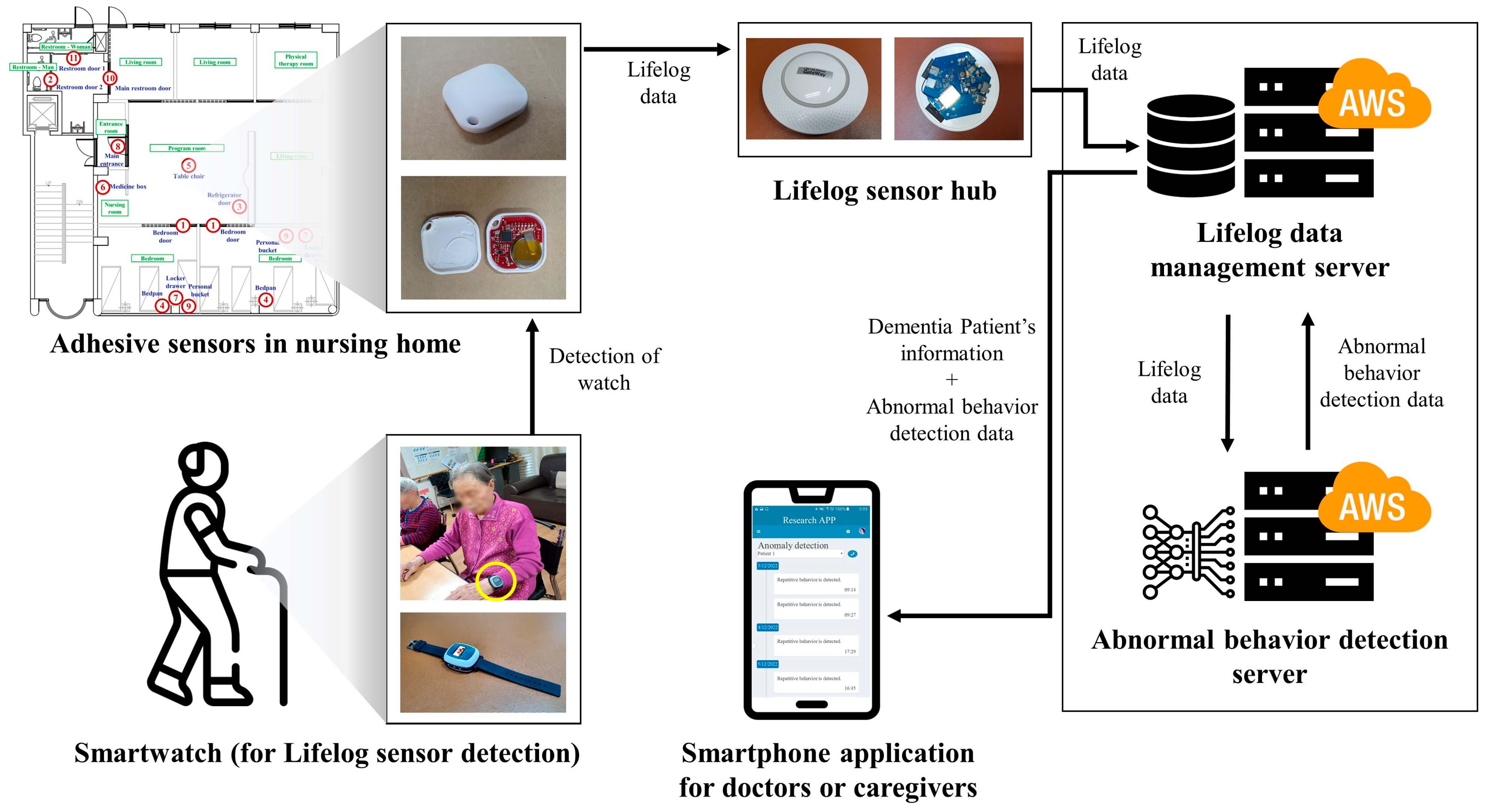
Figure 1. Structure of machine-learning-based system for detecting abnormal behavior in dementia patients.
Information 14 00433 g001
Figure 2. The structure of the nursing home where a machine-learning based system was tested for detecting abnormal behavior in dementia patients.
Information 14 00433 g002
Figure 3. Actual photos of adhesive lifelog sensor devices installed in nursing home.
Information 14 00433 g003
Figure 4. Adhesive lifelog sensor structure and actual device.
Information 14 00433 g004
Figure 5. Smartwatch structure, actual device, and lifelog sensor hub.
Information 14 00433 g005
Figure 6. Using UMAP for visualization of datasets before and after preprocessing.
Information 14 00433 g006
Figure 7. Confusion matrices for each model.
Information 14 00433 g007
Figure 8. Localization curve graphs for each model.
Information 14 00433 g008
Figure 9. Receiver operating characteristic graphs for each model.
Information 14 00433 g009
Figure 10. Precision–recall curve graphs for each model.
Information 14 00433 g010
Table 1. Related works on abnormal behavior detection using machine learning.
Study (Year)DatasetModelAccuracy
Kuppusamy, P. et al. [6] (2022)UCF-Crime [7], UCSD [8]CNN [9]99.5%
Niu, Z. et al. [10], (2023)NSL-KDD [11], KDD Cup 99 [12]ADESSA [10]99.2%
Wang, J. et al. [13] (2019)Human behavior video dataset [13]CNN [9], LSTM [14]92.5%
Han R. et al. [15] (2023)Host behavior data [15]KNN [18], NB [19], RF [20], AE [21], MemAE [22]98.3%
Huang, C. et al. [23] (2021)UCSD [24], CUHK Avenue [25], ShanghaiTech [26]MemAE [22], TAC-Net [23], ISTL [27], sRNN-AE [28]98.1%
Chen, G. et al. [29] (2020)NeuroAED [29]EMST [29], SR [30], K-SVD [31]95.8%
Li, G. et al. [32] (2022)Time series dataset [32]LSTM [14], AE [21]91.7%
Table 2. Location and details of adhesive lifelog sensor devices.
Sensor NumberLocationFurniture or Appliances
1BedroomBedroom door
2Restroom—ManRestroom door 2
3Program roomRefrigerator door
4BedroomBedpan
5Program roomTable chair
6Nursing roomMedicine box
7BedroomLocker drawer
8Main entranceMain entrance
9BedroomPersonal bucket
10RestroomMain restroom door
11Restroom—WomanRestroom door 1
Table 3. Examples of abnormal behaviors in dementia patients.
Abnormal BehaviorsDescription
WanderingWalking aimlessly and getting lost, especially in familiar surroundings
FallsLosing balance and falling, often leading to injury
Sleep disturbancesDifficulty falling asleep or staying asleep
Delusions/Hallucinationsseeing, hearing, or believing things that are not real
Agitation and aggressionVerbal or physical outbursts, including hitting, biting, or kicking, often in response to frustration or confusion
Repetitive questioning/behaviorsAsking the same question or doing the same action repeatedly
Eating disturbances (overeating, pica, anorexia)Eating too much or too little, or eating non-food items, such as paper or dirt
Medication mismanagementTaking too much medication or taking medication improperly
Hoarding/Inappropriate behaviors (including hoarding objects or engaging in socially inappropriate or unhygienic behaviors)Collecting or hoarding items or engaging in behavior that is socially inappropriate or unhygienic
Table 4. Lifelog dataset with labeled abnormal behaviors.
DateTimeSensor NumbersLabel
1234567891011
15 November 202207:100000003037001
15 November 202207:110000010705000
15 November 202207:120000001709000
15 November 202207:14006000000000
Table 5. Preprocessed lifelog dataset.
DatetimeSensor NumbersLabelTAMaxAMeanASA
111
15 November 2022 07:1000121.015.03.8187.723
15 November 2022 07:1100024.024.04.36410.854
15 November 2022 07:1200040.037.07.36317.023
15 November 2022 07:1500022.010.04.0006.842
15 November 2022 07:1600026.017.04.7279.234
Table 6. Experimental setup and model parameters.
ModelParameters
KNNn_neighbors: 5
weights: ‘uniform’
algorithm: ‘auto’
RFn_estimators: 100
max_depth: None
min_samples_split: 2
min_samples_leaf: 1
max_features: ‘auto’
bootstrap: True
LRC: 1.0
penalty: ‘l2’
solver: ‘lbfgs’
max_iter: 100
DTcriterion: ‘gini’
splitter: ‘best’
max_depth: None
min_samples_split: 2
min_samples_leaf: 1
SVMC: 1.0
kernel: ‘rbf’
gamma: ‘scale’
decision_function_shape: ‘ovr’
max_iter: -1
MLPhidden_layer_sizes: 1 layer of 100 neurons (100)
activation: ‘relu’
solver: ‘adam’
alpha: 0.0001
batch_size: ‘auto’
learning_rate: ‘constant’
max_iter: 200
random_state: 42
Table 7. Confusion matrix.
Actual Values
PositiveNegative
Predicted ValuesPositiveTPFP
NegativeFNTN
Table 8. Performance evaluation results by model.
ModelAccuracyPrecisionRecallF1 Score
012012012
LR0.97940.980.48110.080.890.990.130.94
DT0.999711110.99110.991
RF0.9959110.9910.810.9910.890.99
SVM0.96610.9701100.140.9800.24
KNN0.98710.990.910.9710.490.880.990.640.92
MLP0.9999111111111
Disclaimer/Publisher’s Note: The statements, opinions and data contained in all publications are solely those of the individual author(s) and contributor(s) and not of MDPI and/or the editor(s). MDPI and/or the editor(s) disclaim responsibility for any injury to people or property resulting from any ideas, methods, instructions or products referred to in the content.