Article

On Isotropy of Multimodal Embeddings

by
Kirill Tyshchuk
1,*,†,
Polina Karpikova
1,†,
Andrew Spiridonov
1,†,
Anastasiia Prutianova
1,
Anton Razzhigaev
1,2 and
Alexander Panchenko
1,2,*
1
Center of Artificial Intelligence Technology (CAIT), Skolkovo Institute of Science and Technology (Skoltech), 121205 Moscow, Russia
2
Artificial Intelligence Research Institute (AIRI), 121170 Moscow, Russia
*
Authors to whom correspondence should be addressed.
These authors contributed equally to this work.
Information 2023, 14(7), 392; https://doi.org/10.3390/info14070392
Submission received: 21 April 2023 / Revised: 18 June 2023 / Accepted: 22 June 2023 / Published: 10 July 2023
(This article belongs to the Special Issue Information Visualization Theory and Applications)

Abstract

:
Embeddings, i.e., vector representations of objects, such as texts, images, or graphs, play a key role in deep learning methodologies nowadays. Prior research has shown the importance of analyzing the isotropy of textual embeddings for transformer-based text encoders, such as the BERT model. Anisotropic word embeddings do not use the entire space, instead concentrating on a narrow cone in such a pretrained vector space, negatively affecting the performance of applications, such as textual semantic similarity. Transforming a vector space to optimize isotropy has been shown to be beneficial for improving performance in text processing tasks. This paper is the first comprehensive investigation of the distribution of multimodal embeddings using the example of OpenAI’s CLIP pretrained model. We aimed to deepen the understanding of the embedding space of multimodal embeddings, which has previously been unexplored in this respect, and study the impact on various end tasks. Our initial efforts were focused on measuring the alignment of image and text embedding distributions, with an emphasis on their isotropic properties. In addition, we evaluated several gradient-free approaches to enhance these properties, establishing their efficiency in improving the isotropy/alignment of the embeddings and, in certain cases, the zero-shot classification accuracy. Significantly, our analysis revealed that both CLIP and BERT models yielded embeddings situated within a cone immediately after initialization and preceding training. However, they were mostly isotropic in the local sense. We further extended our investigation to the structure of multilingual CLIP text embeddings, confirming that the observed characteristics were language-independent. By computing the few-shot classification accuracy and point-cloud metrics, we provide evidence of a strong correlation among multilingual embeddings. Embeddings transformation using the methods described in this article makes it easier to visualize embeddings. At the same time, multiple experiments that we conducted showed that, in regard to the transformed embeddings, the downstream tasks performance does not drop substantially (and sometimes is even improved). This means that one could obtain an easily visualizable embedding space, without substantially losing the quality of downstream tasks.

1. Introduction

The automatically learned vector representations (embeddings) of various objects, such as texts, images, and graphs are at the heart of almost every successful deep learning model. Therefore, various researchers have tried to analyze their statistical properties and suggest transformations for improving the quality of downstream tasks. What is more, such dense vector representations are a natural common ground for representing objects of various modalities in the same space. For instance, a text fragment describing an animal, such as a llama, should be topologically close to a correct image of a llama in such a space.
Prior research has shown the importance of analyzing the isotropy of textual embeddings for transformer-based text encoders, such as the BERT model [1,2]. Anisotropic word embeddings do not use the entire space, instead concentrating on a narrow cone in such a pretrained vector space, negatively affecting the performance of applications, such as textual semantic similarity. Transforming a vector space to optimize isotropy has been shown to be beneficial for improving performance in text processing tasks [3,4]. This paper is the first comprehensive investigation of the distribution of multimodal embeddings using the example of OpenAI’s CLIP [5] pretrained model. Our initial efforts focused on measuring the alignment of image and text embedding distributions, with an emphasis on their isotropic properties [1,6,7,8].
OpenAI’s CLIP [5] serves as a compelling example of such a multimodal model with zero-shot and open-set classification capabilities. This model excels by learning meaningful embeddings of images and text (potentially multilingual) in a shared latent space, as shown in the semantic visualization of the image embeddings space in Figure 1. In this work, we claim that to truly understand the CLIP’s mechanism, its strengths, and limitations it is essential to study the distribution of these embeddings.
In this article, we dive deep into several important aspects of CLIP’s embedding space, aiming to uncover its structure and evaluate its features through visualization and quantitative analysis. In our study, we optimize the isotropy and modality alignment of CLIP embeddings, therefore making them more visualizable. Meanwhile, our multiple experiments showed that the performance in downstream tasks does not drop substantially (and is sometimes even improved) with this kind of transformed embeddings. This means that one could obtain (using the methods described in this article) easily visualizable embeddings and not lose quality for downstream tasks.
At the same time, we investigate the potential of isotropy restoration methods to improve the quality of the CLIP model. We also consider the role of linear algebra matrix approximation and dimensionality reduction techniques in boosting CLIP’s zero-shot abilities. Finally, we analyze the multilingual versions of CLIP, studying the alignment of text embeddings in different languages. Through this investigation, our goal was to gain a comprehensive understanding of the structure, isotropy, enhancement methods, zero-shot capabilities, and multilingual alignment within the CLIP model.
The key findings of our investigation can be summarized as follows:
  • The distribution of CLIP embeddings is not centered, therefore forming a cone, but they have a high level of isotropy in a local sense [8];
  • Both CLIP image and text encoders generate embeddings that are located in a cone not just after training, but also right at initialization, even when layer biases are set to zero;
  • While most elementary linear algebra methods aimed at increasing the isotropy of embeddings do not substantially improve CLIP’s zero-shot classification performance, certain dimensionality reduction and distribution alignment techniques may nonetheless provide potential enhancements;
  • When mBERT [9] and XLM-RoBERTa [10] are used as text encoders, CLIP produces multilingual text embeddings that correlate with their corresponding image embeddings closely, despite not using any image information during training.

2. Literature Review

The issue of how transformers [11] utilize their embedding space has been the subject of inquiry in various studies. Numerous investigations into the embedding space of transformer models suggest that the distribution of contextual representations is highly anisotropic. An isotropic distribution or point cloud is the one that appears similar in all directions in space. However, this characteristic is generally not observed in the embeddings distributions learned by transformers. Instead, these distributions tend to be stretched in a specific direction and are confined within a narrow cone around it. For example, in Gao et al. [1], authors particularly underline this phenomenon, calling it the the Representation Degeneration Problem. They hypothesize that it limits the representation power of word embeddings because they are less diverse than they could be; when all of the embeddings are inside a narrow cone, all of the cosine similarities are positive or even close to 1 in extreme cases. This is also the reason why classifiers based on the cosine similarity have small margins, which could lead to poor generalization. The authors attribute this problem to the gradients of the likelihood loss pushing the embeddings in the same direction during training. Finally, the authors show that regularization aimed for restoring isotropy can improve the quality of the model. Techniques with a similar goal are also developed in other works [6,7]. In Su et al. [4], authors propose to use the whitening procedure to restore isotropy of the BERT embeddings, which leads to better performance of their cosine similarity scores for the Semantic Similarity tasks. It also enables the reduction in the dimension of the embeddings. Li et al. [3] show that anisotropy hinders the performance of sentence embeddings obtained by BERT and propose making their distribution Gaussian using an additional normalizing flow model.
However, the importance of isotropy in transformer embeddings is disputable. First, the embeddings may be locally isotropic as discovered by Cai et al. [8]. The researchers show that each cluster of the embeddings cloud becomes isotropic after centering. Our research shows that the centering alone already significantly improves the isotropy. This may mean that the embeddings have a non-degenerate, rich and meaningful structure when analyzed using the Euclidean distance, and the apparent anisotropy may be attributed to their distribution being uncentered. Furthermore, Ding et al. [12] report that the isotropy restoration techniques do not bring significant improvement to the models.

3. Method Description

3.1. Visualization, Isotropy, and Transformations

3.1.1. Data Description

We started by precomputing the CLIP embeddings on the COCO [13] dataset. We used the 2014val captions task part of the dataset, containing images and corresponding captions. We computed the visual and text embeddings for two CLIP models, CLIP-ViT-B/32 with a visual transformer backbone and CLIP-RN101 with a ResNet backbone. The findings are similar for all three models, so we present the first one as a sufficient example, CLIP-ViT-B/32.

3.1.2. Isotropy Analysis

We started by analyzing the distributions of cosine similarities between embeddings of random positive (corresponding) and negative (non-corresponding, random) image-text pairs.
Then we visualized the embedding space similarly to the previous works by projecting the data onto the first two SVD components of the embeddings matrix. Note that we intentionally used a linear projection because the non-linear ones may not preserve anisotropy.
To characterize the isotropy of the embedding space, we adopted the I 1 and I 2 isotropy measures from [1,6]. The first measure is defined as
I 1 ( W ) = min v E Z ( v ) max v E Z ( v ) ,
where W is the n × d embeddings matrix with rows w i R d as individual embeddings, Z : R d R + is the partition function Z ( v ) = i = 1 n exp ( v , w i ) , and  E is the set of eigenvectors of W T W . The second measure, defined as
I 2 ( W ) = v E ( Z ( v ) Z ¯ ( v ) 2 ) | E | Z ¯ ( v ) 2
is the sample standard deviation of the partition function Z ( v ) normalized by its average Z ¯ ( v ) . Z should be close to a constant on E if the embedding matrix W is isotropic. This way, I 1 ( W ) [ 0 , 1 ] , I 2 ( W ) 0 , and larger I 1 ( W ) and smaller I 2 ( W ) indicate more isotropic embeddings. For the details, refer to [1,6]. We report the isotropy metrics I 1 and I 2 for various settings. Because CLIP embeddings are trained with cosine similarity loss, which is invariant to scaling, we normalized them before computing any metrics. Another important point is that I 1 and I 2 metrics are not invariant to scaling, so when we analyzed the embeddings after different transformations, we also normalized them to ensure a fair comparison.
Another simpler isotropy metric is the distribution of standard deviations of all of the embedding coordinates. If it is concentrated, then all of the coordinates have an equal contribution to the overall variance, and the embeddings are isotropic.

3.1.3. How to Improve Isotropy

We also articulate the importance of centering for the embeddings analysis. The cosine similarity is not invariant to centering, but it can be expressed in terms of Euclidean distance. For any vectors x , y of unit norm, we have:
cos ( x , y ) = x , y = 1 1 2 x y 2 2
That means that we can study the geometric properties of the cluster of normalized embeddings via Euclidean distance, which is invariant to centering.
We proceed by using the whitening-k transformations from Su et al. [4] to the obtained embeddings distributions. It centers the distribution and makes all of the singular values of the embedding matrix equal to one, which means that the variance is constant in any direction, and the distribution is spherical and isotropic. The k parameter stands for the dimensionality of the obtained representations. The first k SVD (PCA) components of the initial matrix are retained (but their singular values are normalized), and the others are omitted as in the regular PCA dimensionality reduction technique.
Coming up with a novel approach, we employed simple linear algebra methods to align the distribution of image representations with the distribution of their respective caption representations. The most straightforward way to achieve that is to move one of the distributions with a linear transformation. Suppose A is the (normalized) text embedding matrix and B is the (normalized) image embedding matrix. We can find a linear transformation Ω that makes the text representation closer to the corresponding image representations in terms of L 2 norms. Therefore, we aim to minimize A Ω B F 2 , where · F is the Frobenius norm. This is equivalent to finding the least-squares solution to a linear matrix equation A Ω = B and commonly referred to as lstsq in linear algebra packages. However, the arbitrary linear transformation does not preserve the norms of the embeddings, so after the transformation they will no longer be normalized and their pairwise cosine similarities will change. If we wish to avoid that, we can impose the orthogonality constraint on Ω . This way, we can preserve both the normalization and the cosine similarities. Thus, the inner structure of the text embeddings will not change, their distribution will simply be rotated. The problem of minimizing A Ω B F 2 on the set of orthogonal matrices Ω is called the orthogonal Procrustes problem. Moreover, we can see that in the case of normalized embeddings, it is equivalent to maximizing the sum of cosine similarities between the text and image embeddings
A Ω B F 2 = A Ω F 2 + B F 2 2 A Ω , B min Ω
where · , · is the element-wise inner product. As  A Ω and B consist of unit vectors, this is equivalent to
A Ω , B max Ω
which corresponds to maximizing the sum of the cosine similarities between the rows of A Ω and B under the orthogonality constraint on Ω . Both LSTSQ and orthogonal Procrustes problems are implemented in the commonly used linear algebra packages. For example, we used Torch and SciPy implementations of these functions torch-linalg-lstsq (https://pytorch.org/docs/stable/generated/torch.linalg.lstsq.html#torch-linalg-lstsq, accessed on 21 June 2023), scipy-linalg-orthogonal-procruste (https://docs.scipy.org/doc/scipy/reference/generated/scipy.linalg.orthogonal_procrustes.html#scipy-linalg-orthogonal-procruste, accessed on 21 June 2023). The solutions are computed efficiently in less than a second, even for moderately-sized 40,000 × 512 input matrices.

3.1.4. Evaluation Settings

We tested the aforementioned approaches using three different conditions. Under the first condition, the parameters of the transformations were computed (fitted, trained) on the COCO embeddings and then applied to CIFAR. This can be viewed as an extension to the CLIP training with further testing of the effect of this procedure on its generalization. Under the second condition, we computed the parameters on the CIFAR train embeddings and tested them on the CIFAR test ones. This corresponds to learning a kind of domain adaptation. Under the third condition, we performed training on the part of CIFAR, corresponding to 50 random classes (we call them known) and performed tests on the other instances. This also corresponds to domain adaptation (adapting the CLIP embeddings for CIFAR classification) but it is closer to the zero-shot paradigm than the second condition.

3.2. Multilingual CLIP

Multilingualism in CLIP can be achieved by training the text encoder with a corpus of any language (i.e., there is ruCLIP (https://github.com/ai-forever/ru-clip, accessed on 21 June 2023) for Russian image–text pairs). However, this is not optimal. A more natural and widely-used way is to take multilingual BERT as a text encoder and train it in a CLIP setting using captions in a single reference language (standard CLIP training). This text encoder is then fine-tuned with the objective of text embeddings alignment on a parallel caption corpus (for example, minimizing MSE loss between human-generated translations). The question is, how good are the final multilingual textual embeddings in the CLIP space? How can we measure it?
To address this, we used the WikiCap [14] dataset and a readily available multilingual CLIP implementation (https://github.com/FreddeFrallan/Multilingual-CLIP, accessed on 21 June 2023) to compute the corresponding embeddings and inspect them visually and quantitatively. The dataset presents French–English, Russian–English, and German–English caption pairs along with the corresponding images from Wikipedia. To visualize the position of embeddings as point clouds, we use a non-linear projection method UMAP [15], which aims to preserve local distances and build a low-dimensional graph representation of the original high-dimensional data. UMAP also tends to preserve the relative positions of clusters in data, which perfectly suits our task.

Evaluating the Quality of Embeddings

To test the quality of the obtained representations, we measured the contrastive loss used in the CLIP training on the COCO images and captions as the first step. This is the most straightforward way to see if the similarity between the corresponding embedding pairs is higher than for the random ones. We split the dataset into the train part used to compute the parameters of the embedding transformation and the test part for a more rigorous evaluation of the generalization.
One of the most notable applications of CLIP is performing classification without the need for prior training on specific classes. Thus, secondly, we used the CIFAR-100 [16] to measure the accuracy of zero-shot classification with CLIP using the following method. In our approach, we initially generate a corresponding text for each label. Subsequently, the predicted label is determined based on the text that exhibits the closest cosine distance between its embedding and the embedding of an image to be classified. To achieve optimal accuracy, we experimented with various prompts and selected those that yielded the highest accuracy. We utilized the template “low-resolution photo of a 〈fine class name〉” for English captions, while for Russian ones, we employed the template “изoбражение 〈fine class name〉”. Additionally, we precomputed the embeddings for the CIFAR-100 dataset and divided them into train and test sets. One of the transformations that we applied to CLIP embeddings, was dimensionality reduction through principal component analysis (PCA) to achieve better zero-shot classification performance. The idea was that text embeddings, that were corresponding to a picture, could be redundant. For instance, the phrase “orange cat on the green grass” could be reduced to “cat” for classification purposes. However, the phase could potentially be reduced to “grass”, causing errors. We “trained” the transformation on the COCO dataset and applied it to CIFAR-100 text and images.
In addition to analyzing the zero-shot classification ability of a model, it is more common to study its representation learning capabilities. There are many ways to evaluate the quality of representations. We used the linear probe method, fitting a linear classifier on the representation extracted from the model and measuring its performance on various datasets.

4. Results

4.1. Visualization and Isotropy Metrics

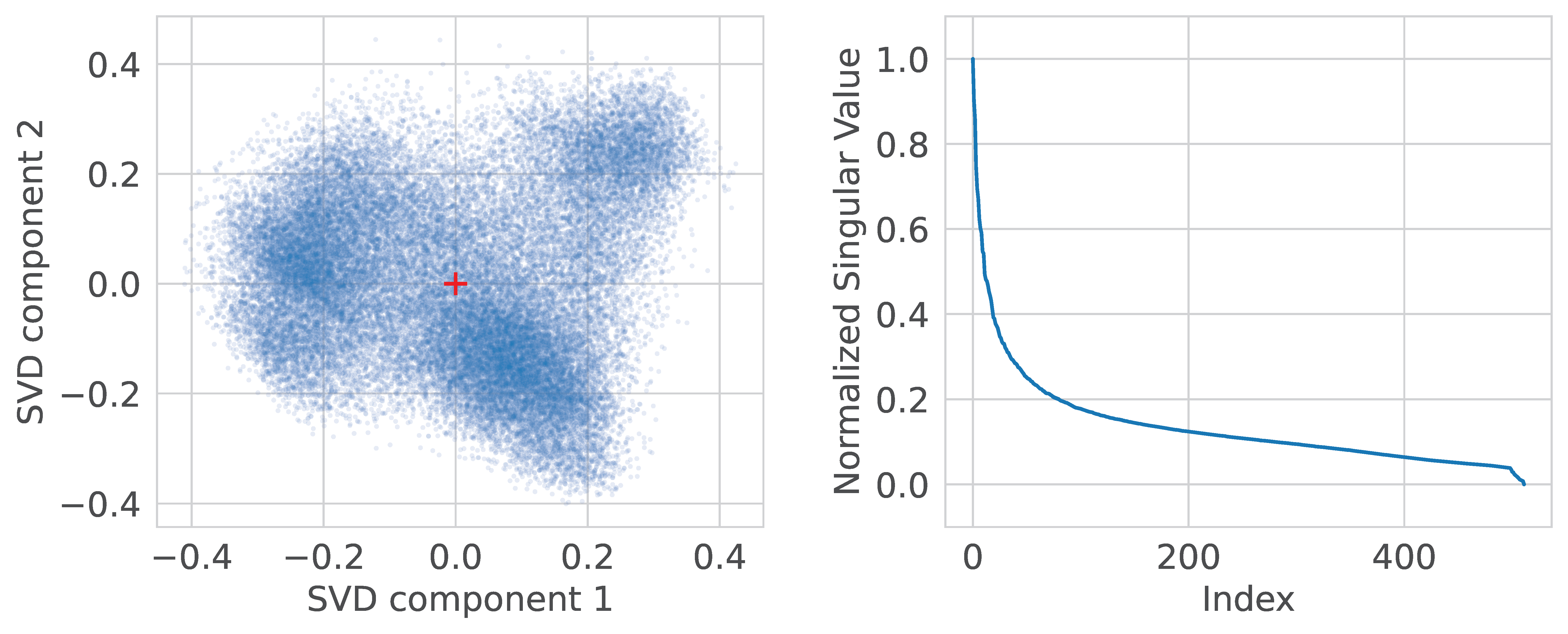
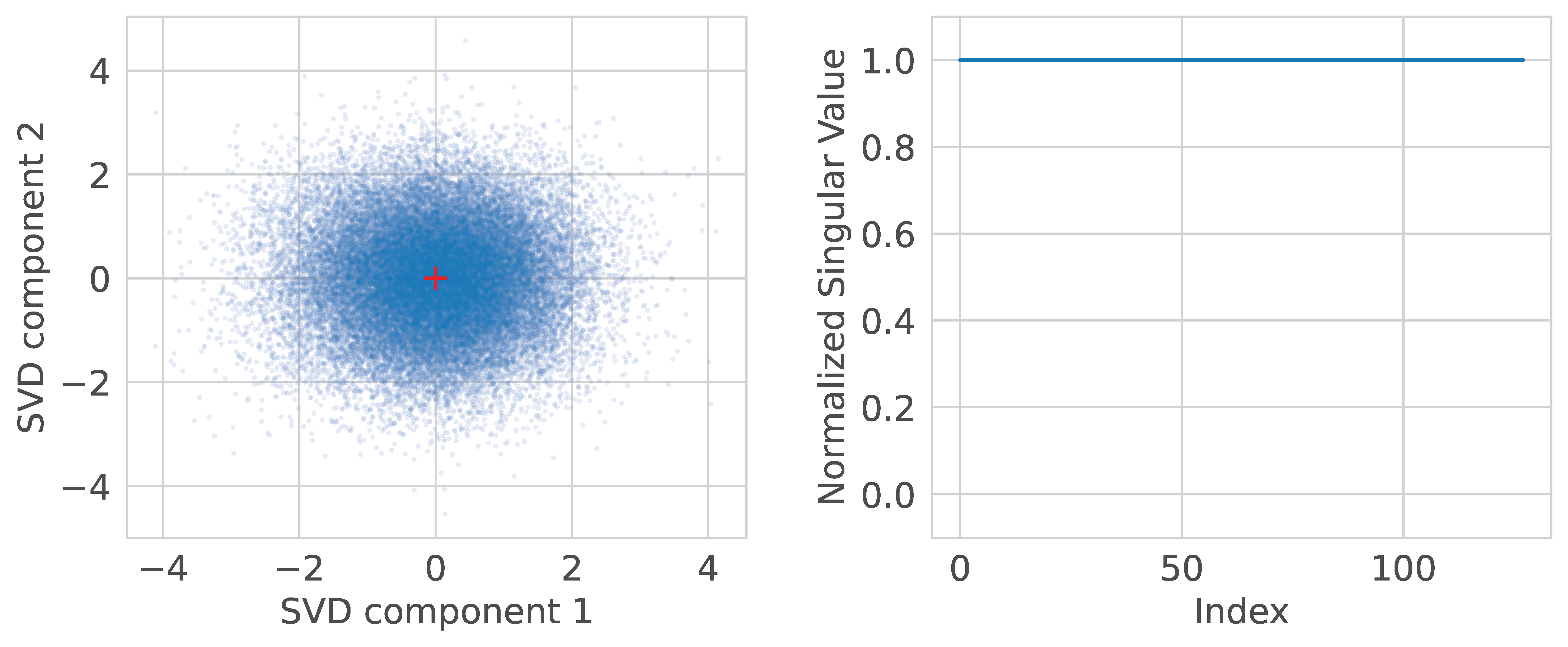
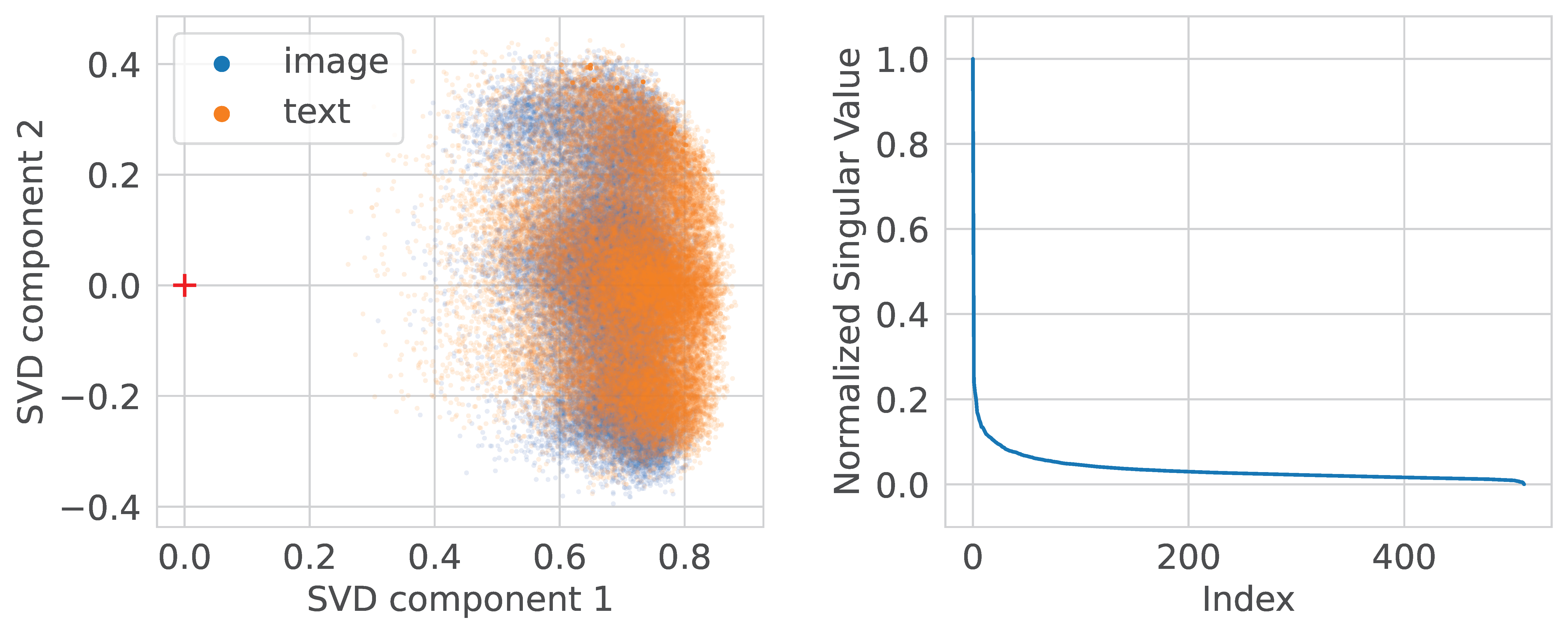
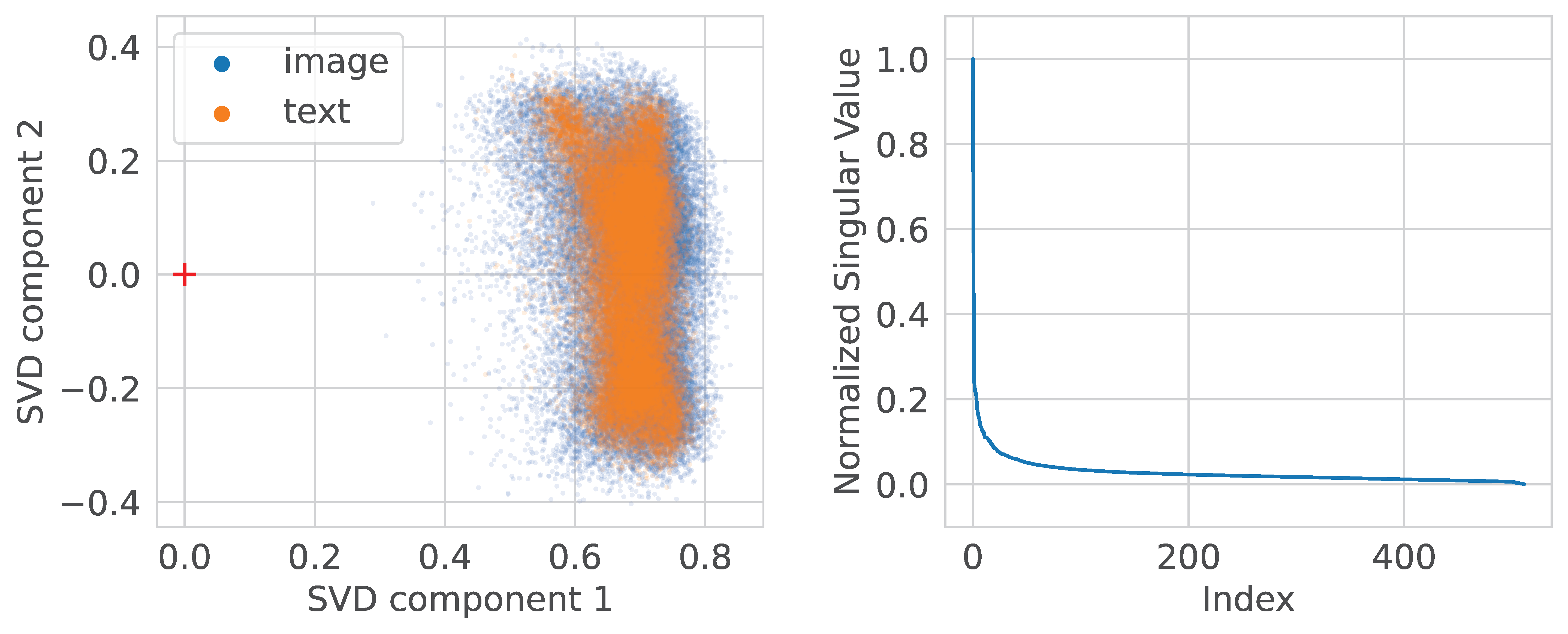
We present the visualization of the CLIP embeddings using Singular Value Decomposition (SVD). The image embeddings, after normalization, are situated within a cone starting from the origin, as depicted in Figure 2. The pairwise cosine similarities between these embeddings are all positive. However, when the embeddings are centered (Figure 3), we observe a more or less isotropic distribution, characterized by a slower decay of singular values. This suggests that, even when viewed as a single cluster, the embeddings exhibit local isotropy. This observation is further supported by the isotropy metrics presented in Table 1. It can be speculated that the increase in isotropy from [8] can be attributed to the centering of each cluster, rather than the clustering itself.
Figure 4 illustrates the image embeddings after whitening-128. Note the spherical shape of the distribution and the flat singular values plot.
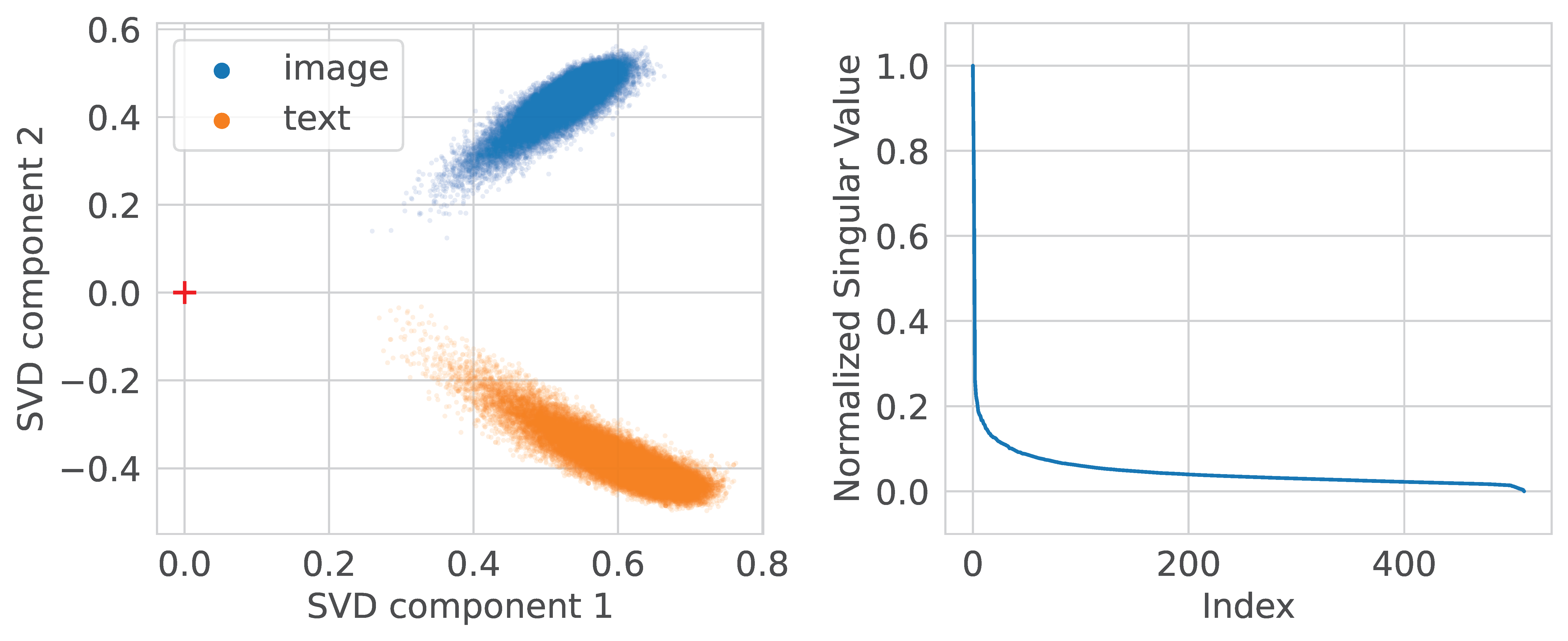
It is important to note that the embeddings in CLIP are linearly separable rather than mixed. This may seem counterintuitive, but the CLIP contrastive loss does not explicitly restrict this. For instance, if we introduce a coordinate that consistently has a value of 0.1 for image embeddings and + 0.1 for text embeddings, all dot products decrease by 0.01 , and the norms do not change significantly. Hence, the cross-entropy loss within the contrastive loss remains majorly unchanged. However, such a dimension would provide no meaningful information and could potentially have negative implications for certain applications that rely on close proximity between image and text embeddings. Furthermore, we conducted experiments to see if the image and text embeddings were linearly separated. By training a logistic regression model and a linear Support Vector Classifier (SVC), we achieved an accuracy of 1.0 in both cases, confirming that the embeddings are indeed linearly separated.
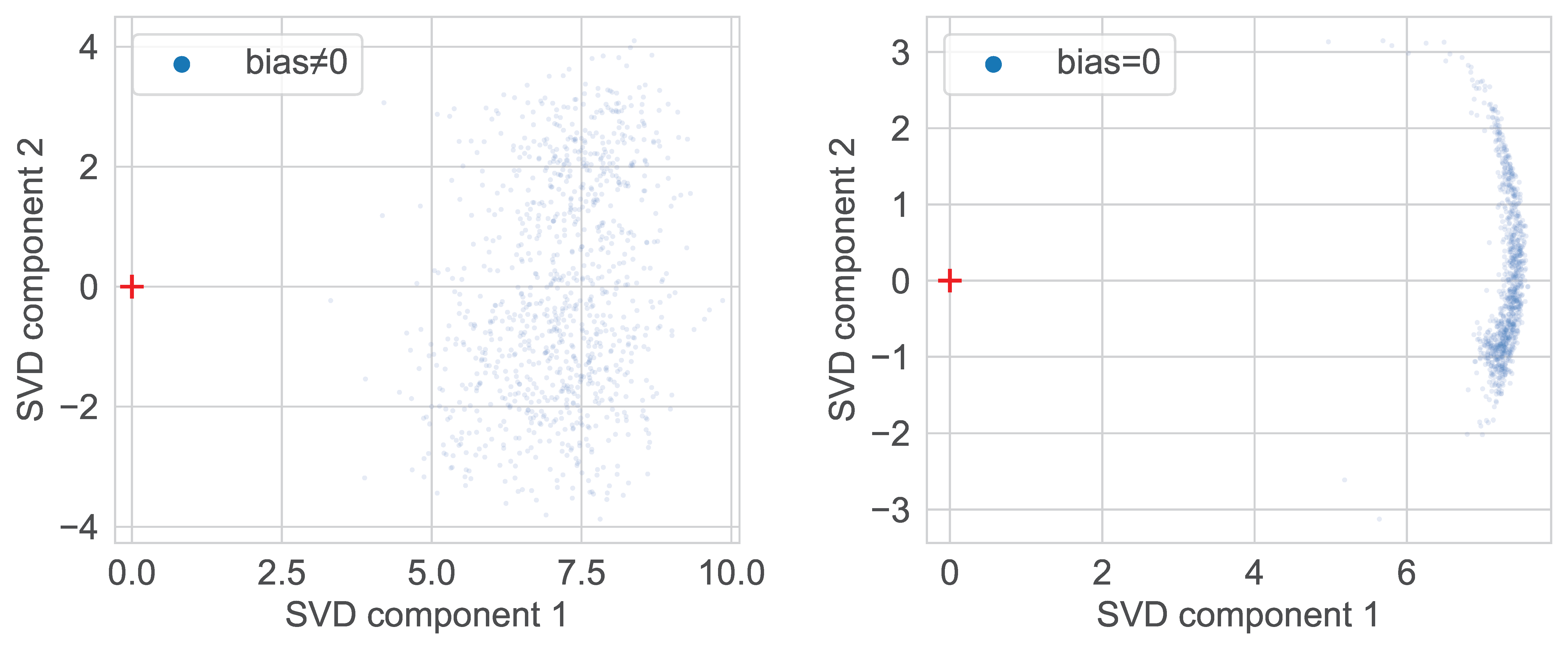
To understand the anisotropy of embeddings, we checked their initial distribution at network initialization. The results are shown in Figure 5, Figure 6 and Figure 7. It turns out that right after the initialization, both image and text embeddings are offset from the origin and hence bounded by a cone. To ensure this is not due to bias present in neural network layers, we set all biases to zero, and the effect still persisted. We leave it to future work to analyze this property of random initialization of CLIP’s architecture in a probabilistic framework similar to Neural Tangent Kernel [17].
Figure 8 shows visualization of the joint image and text embeddings distribution for trained CLIP.

4.2. Procrustes and LSTSQ Transformations

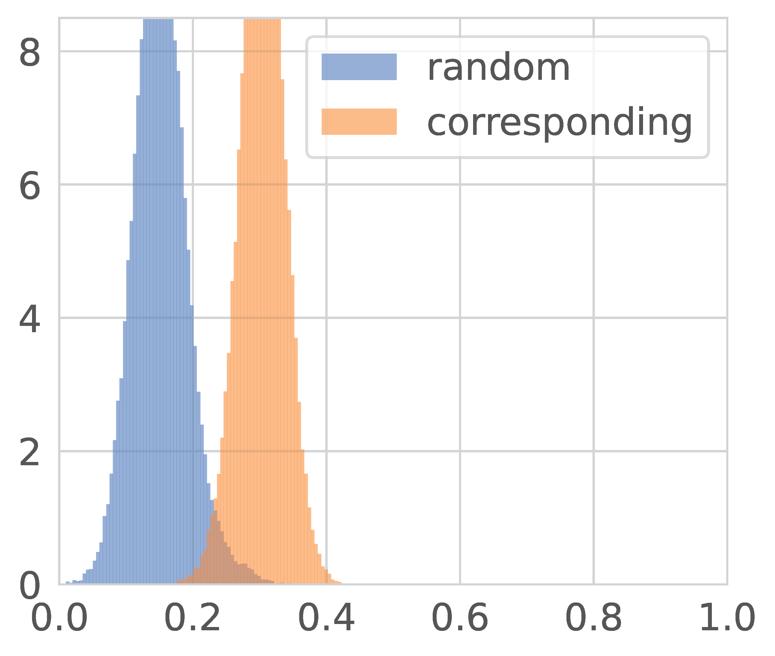
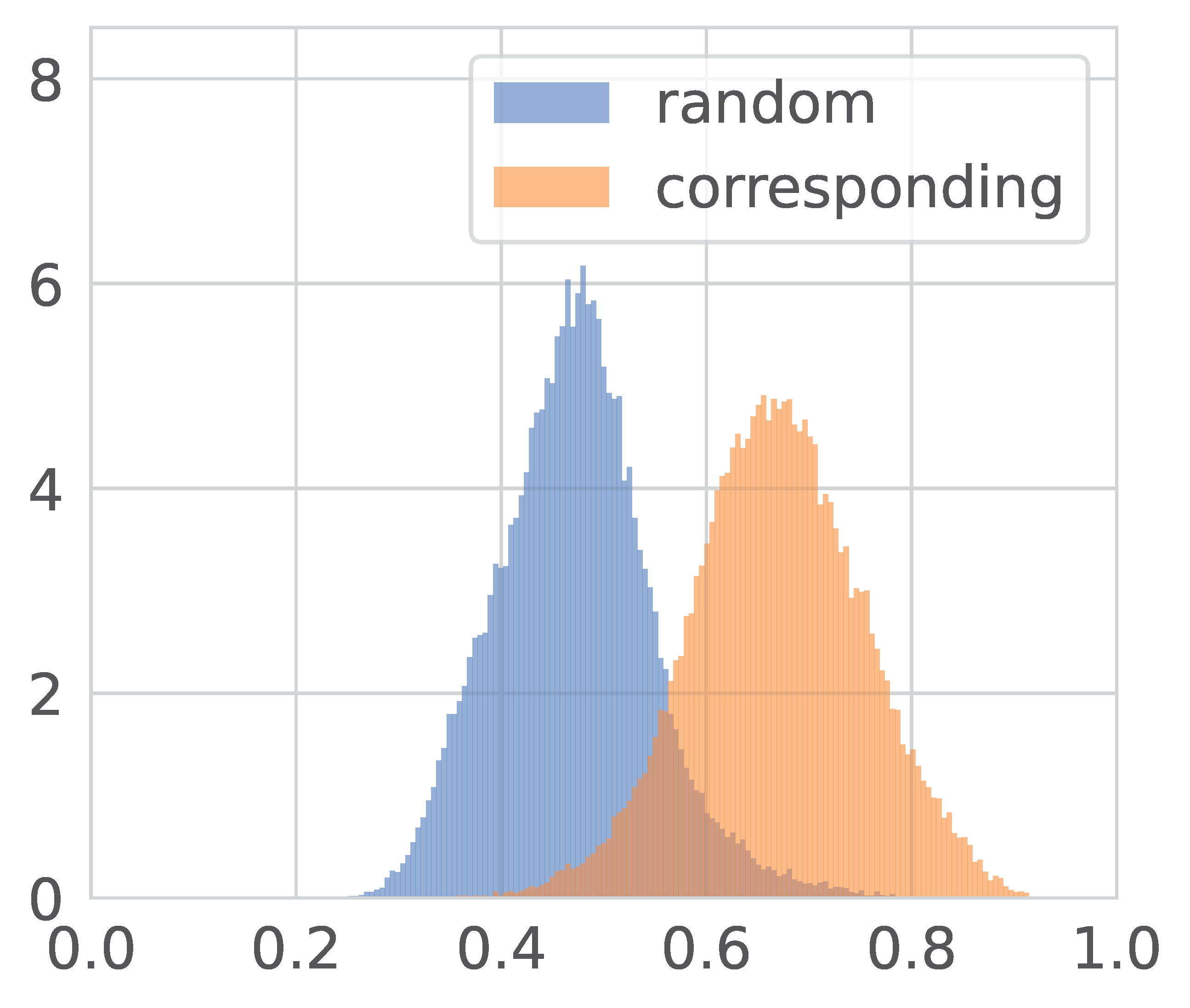
We present the results of the experiments aimed at aligning image and text representation distributions. In Figure 9, Figure 10 and Figure 11, the distributions of cosine similarities between random images and texts and between corresponding ones are depicted. CLIP is trained to separate those distributions.
Note that the similarities are much larger after the Procrustes and LSTSQ transformations. The gap between their peaks is also greater, but the overlap is slightly higher.
As we saw in Figure 8, although the original text and image embeddings distributions are close, they almost do not intersect, while the transformations fix this. The overlap after the LSTSQ transformation is more prominent than after the Procrustes.
Figure 12 and Figure 13 display the joint image and text representation distributions after the Procrustes and LSTSQ transformations correspondingly. Note how the distributions are better mixed and how LSTSQ warped the text distribution.

4.3. CLIP Loss Evaluation

In Table 2, we present the CLIP loss evaluation after different embedding transformations. We hypothesize that we were unable to improve it with SGD-free methods because the CLIP embeddings are already well-optimized for this objective.

4.4. CIFAR-100 Zero-Shot Accuracy

Here, we evaluate how our transformations affect the zero-shot capabilities of the CLIP embeddings. The results are shown in Table 3. Note that the experiment with the whitening parameters computed on the test sample is not entirely fair. Still, the only simplification is that during the test all the pictures are available to us at once, not just one picture at a time. Furthermore, note that the training accuracy does not drop much with the reduction in the number of components from 128 to 64 in whitening on CIFAR, but on COCO the difference is significant. This indicates that the parameters of the transformations are sensitive to the dataset on which they are computed. PCA-450 refers to performing a dimensionality reduction down to 450 components via PCA, and the results show that it is possible to preserve or even slightly improve the zero-shot capabilities by eliminating the least informative dimensions. PCA-90 results were obtained by performing PCA on the 100 text prompts used for classification. We conclude that such dimensionality reduction is basically enough to preserve the subspace of prompts for the accuracy not to drop significantly. We additionally tested two other ways to obtain the logits using a pair of (unnormalized) transformed embeddings: dot-product x , y and negated distance 1 1 2 x y 2 2 , but they yield worse quality.
Finally, in Table 4, we present our attempt at CIFAR domain adaptation learned on half the classes and generalized to the other half. The results are negative. This is probably because even if the transformation does align the first 50 class representation vectors, it still has many degrees of freedom to break the other 50, as the overall dimension is 512 or more.
In conclusion, we see that although the Procrustes and LSTSQ transformations change the embeddings significantly, they do not break the CLIP model and even sometimes improve it. This is a convincing proof of concept for applying these transformations for CLIP. They may be incorporated in the training procedure, as they are computationally cheap, or be used as a post-processing step, but with caution.

4.5. Linear Probe Evaluation

We trained a logistic regression classifier using the scikit-learn L-BFGS implementation, with a maximum of 1000 iterations, and reported the corresponding metric on test image embeddings. The results are in Table 5. It is clear that although the dimension of the embeddings was significantly reduced, the information that was necessary for classification, was preserved.

4.6. Semantic Visualization of the Embedding Space

We used T-SNE to compute a two-dimensional visualization of image and text embeddings that respects the high-dimensional (Euclidean) distances. Images are displayed exactly at their embedded location. The result can be seen in Appendix A. The objects of the same class indeed lay nearby. Note that we found the perplexity parameter that is equal to 5 for images and 50 for the texts to be the best. This observation indirectly implies that the text embeddings are located further away from each other, unlike the image ones.

4.7. Multilingual CLIP

To address the question of how multilingual embeddings are distributed we selected Multilingual CLIP with backbones M-BERT-Distil-40 and XLM-Roberta-Large-Vit-B-16Plus as the two most popular models. We present the two-dimensional projections of WikiCaps caption embeddings for these models in Figure 14 and Figure 15 respectfully. It is clear that point clouds are almost identical, which means that the conventional technique of training the multilingual CLIP indeed results in high-quality latent representations, at least in terms of global behaviour and similarity.
We also measured pairwise distances between corresponding latent vectors produced by M-BERT-Distil-40 for parallel text sample and compared those distances with characteristic sizes of the point clouds, as shown in Table 6. The smaller the ratio, the better the alignment of the embedding cloud. Obtained values indicate major structural similarity between embedding different languages, which implies that the quality of those is close to the quality of reference language latents.
In order to further confirm our assumptions that multilingual model has similar textual latent spaces, we calculated the I 1 and I 2 isotropy measures for ruCOCO text embeddings (captions in Russian for COCO dataset), I 1 = 0.81 and I 2 = 0.03 , which is close to the corresponding metrics of the English text embeddings, and conducted an experiment as in Table 3 for the Russian captions as well. The results are in Table 7. Results are matching.

5. Conclusions

Our study empirically shows that CLIP embeddings, exhibiting a noticeable anisotropy, reside within a conical structure. We demonstrate that such a formation emerges at initialization and remains largely unchanged due to the absence of any regularization concerning the absolute location of embeddings in CLIP’s objective function. To fully understand and address this phenomenon, further exploration of the CLIP architecture is needed.
In addition, we found that the isotropy of embeddings can be restored through a simple linear transformation, such as whitening. Furthermore, we identified a method for conducting a learnable linear transformation that, in some cases, can improve performance without incurring substantial computational costs. Although the current scope of these methods is somewhat limited, they could be potentially utilized during or after training to shape an embedding space with desired properties.
The anisotropic characteristic of embeddings extends to the multilingual context as well. In addition, we used the metric properties of the multilingual embeddings to confirm their strong correspondence with the original embeddings. This underscores the consistency of the anisotropic property across diverse linguistic scenarios within the CLIP model.

Author Contributions

Conceptualization, methodology, all authors; supervision, project supervision, A.R., A.P. (Alexander Panchenko); writing K.T., P.K., A.S., A.R., A.P. (Alexander Panchenko); software, investigation, data creation, formal analysis, validation, visualisation, K.T., P.K., A.S., A.P. (Anastasiia Prutianova). The distribution of topics and subtasks is as follows. K.T.: literature review, application of Procrustes and LSTSQ transformations, distribution alignment study, computation of embeddings. A.S.: formal analysis of a simplistic model of transformer embeddings at initialization, methodology and experiment code for multilingual model analysis, image-based visualizations. P.K.: visualization of embedding point cloud projections for majority of methods, image-based visualizations, linear probe and few-shot evaluations, article review and editing. A.P. (Anastasiia Prutianova): dimensionality reduction experiments, isotropy metrics implementation. All authors have read and agreed to the published version of the manuscript.

Funding

This work was supported by Ministry of Science and Higher Education grant No. 075-10-2021-068.

Data Availability Statement

Code and data to reproduce the experiments presented in this article are available openly online at: https://github.com/s-nlp/isotropy, accessed on 21 June 2023.

Conflicts of Interest

The authors declare no conflict of interest.

Appendix A. Semantic Visualization

Please see semantic visualisations of CLIP’s text and image embeddings on the next pages.
Figure A1. Semantic visualisation of image embeddings aligned with textual embeddings below via Procrustes.
Information 14 00392 g0a1
Figure A2. Semantic visualisation of text embeddings aligned with image embeddings above via Procrustes.
Information 14 00392 g0a2

References

  1. Gao, J.; He, D.; Tan, X.; Qin, T.; Wang, L.; Liu, T. Representation Degeneration Problem in Training Natural Language Generation Models. In Proceedings of the 7th International Conference on Learning Representations, ICLR 2019, New Orleans, LA, USA, 6–9 May 2019. [Google Scholar]
  2. Fuster Baggetto, A.; Fresno, V. Is anisotropy really the cause of BERT embeddings not being semantic? In Proceedings of the Findings of the Association for Computational Linguistics: EMNLP 2022, Abu Dhabi, United Arab Emirates, 20 December 2022; pp. 4271–4281. [Google Scholar]
  3. Li, B.; Zhou, H.; He, J.; Wang, M.; Yang, Y.; Li, L. On the Sentence Embeddings from Pre-trained Language Models. In Proceedings of the 2020 Conference on Empirical Methods in Natural Language Processing (EMNLP), Online, 16–20 November 2020; pp. 9119–9130. [Google Scholar] [CrossRef]
  4. Su, J.; Cao, J.; Liu, W.; Ou, Y. Whitening Sentence Representations for Better Semantics and Faster Retrieval. arXiv 2021, arXiv:2103.15316. [Google Scholar]
  5. Radford, A.; Kim, J.W.; Hallacy, C.; Ramesh, A.; Goh, G.; Agarwal, S.; Sastry, G.; Askell, A.; Mishkin, P.; Clark, J.; et al. Learning Transferable Visual Models From Natural Language Supervision. In Proceedings of the 38th International Conference on Machine Learning, PMLR, Virtual, 18–24 July 2021; Meila, M., Zhang, T., Eds.; Proceedings of Machine Learning Research. Volume 139, pp. 8748–8763. [Google Scholar]
  6. Wang, L.; Huang, J.; Huang, K.; Hu, Z.; Wang, G.; Gu, Q. Improving neural language generation with spectrum control. In Proceedings of the International Conference on Learning Representations, Addis Ababa, Ethiopia, 26–30 April 2020. [Google Scholar]
  7. Zhou, W.; Lin, B.; Ren, X. IsoBN: Fine-Tuning BERT with Isotropic Batch Normalization. In Proceedings of the AAAI Conference on Artificial Intelligence, Virtually, 2–9 February 2021; Volume 35, pp. 14621–14629. [Google Scholar] [CrossRef]
  8. Cai, X.; Huang, J.; Bian, Y.; Church, K. Isotropy in the contextual embedding space: Clusters and manifolds. In Proceedings of the International Conference on Learning Representations, Virtual Event, 3–7 May 2021. [Google Scholar]
  9. Devlin, J.; Chang, M.; Lee, K.; Toutanova, K. BERT: Pre-training of Deep Bidirectional Transformers for Language Understanding. In Proceedings of the 2019 Conference of the North American Chapter of the Association for Computational Linguistics: Human Language Technologies, NAACL-HLT 2019, Minneapolis, MN, USA, 2–7 June 2019; Burstein, J., Doran, C., Solorio, T., Eds.; Association for Computational Linguistics; Long and Short Papers. pp. 4171–4186. [Google Scholar] [CrossRef]
  10. Conneau, A.; Khandelwal, K.; Goyal, N.; Chaudhary, V.; Wenzek, G.; Guzmán, F.; Grave, E.; Ott, M.; Zettlemoyer, L.; Stoyanov, V. Unsupervised Cross-lingual Representation Learning at Scale. In Proceedings of the 58th Annual Meeting of the Association for Computational Linguistics, ACL 2020, Online, 5–10 July 2020; Jurafsky, D., Chai, J., Schluter, N., Tetreault, J.R., Eds.; Association for Computational Linguistics. pp. 8440–8451. [Google Scholar] [CrossRef]
  11. Vaswani, A.; Shazeer, N.; Parmar, N.; Uszkoreit, J.; Jones, L.; Gomez, A.N.; Kaiser, L.; Polosukhin, I. Attention is All you Need. In Proceedings of the Advances in Neural Information Processing Systems 30: Annual Conference on Neural Information Processing Systems 2017, Long Beach, CA, USA, 4–9 December 2017; Guyon, I., von Luxburg, U., Bengio, S., Wallach, H.M., Fergus, R., Vishwanathan, S.V.N., Garnett, R., Eds.; pp. 5998–6008. [Google Scholar]
  12. Ding, Y.; Martinkus, K.; Pascual, D.; Clematide, S.; Wattenhofer, R. On Isotropy Calibration of Transformer Models. arXiv 2021, arXiv:2109.13304. [Google Scholar] [CrossRef]
  13. Lin, T.Y.; Maire, M.; Belongie, S.; Hays, J.; Perona, P.; Ramanan, D.; Dollár, P.; Zitnick, C. Microsoft COCO: Common Objects in Context. arXiv 2014, arXiv:1405.0312. [Google Scholar] [CrossRef] [Green Version]
  14. Schamoni, S.; Hitschler, J.; Riezler, S. A dataset and reranking method for multimodal MT of user-generated image captions. In Proceedings of the 13th Conference of the Association for Machine Translation in the Americas (Volume 1: Research Track), Boston, MA, USA, 17–21 March 2018; pp. 140–153. [Google Scholar]
  15. McInnes, L.; Healy, J. UMAP: Uniform Manifold Approximation and Projection for Dimension Reduction. arXiv 2018, arXiv:1802.03426. [Google Scholar]
  16. Krizhevsky, A.; Nair, V. Cifar-100 (canadian institute for advanced research). 30 [65] Alex Krizhevsky, Ilya Sutskever, and Geoffrey E Hinton. Imagenet classification with deep convolutional neural networks. Adv. Neural Inf. Process. Syst. 2012, 25, 26. [Google Scholar]
  17. Jacot, A.; Gabriel, F.; Hongler, C. Neural tangent kernel: Convergence and generalization in neural networks. Adv. Neural Inf. Process. Syst. 2018, 31, 8580–8589. [Google Scholar]
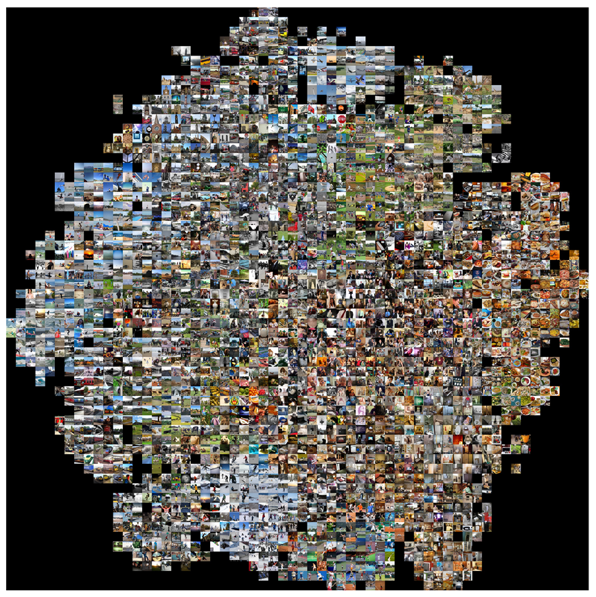
Figure 1. Semantic visualization of image embeddings.
Information 14 00392 g001
Figure 2. CLIP image embeddings distribution and singular values. Note that the embeddings are not centered, so they are located in a cone (with the vertex at the origin). The first SVD component captures the shift from the origin. Fast singular value decay indicates anisotropy. I 1 = 0.84 , I 2 = 0.03 .
Information 14 00392 g002
Figure 3. Centered CLIP image embeddings distribution and singular values. Note a slower singular value decay. I 1 = 0.99 , I 2 = 0.00 .
Information 14 00392 g003
Figure 4. Whitened CLIP image embeddings distribution and singular values. All singular values are equal. I 1 = 0.99 , I 2 = 0.00 .
Information 14 00392 g004
Figure 5. CLIP-RN101 image embeddings distribution computed with (left) or without (right) bias for freshly initialized model (inputs are drawn from COCO-caption-2015).
Information 14 00392 g005
Figure 6. CLIP-ViT-B/32 image embeddings distribution computed with (left) or without (right) bias for freshly initialized model (inputs are drawn from COCO-caption-2015).
Information 14 00392 g006
Figure 7. CLIP text embeddings distribution computed with (left) or without (right) bias for freshly initialized model (inputs are drawn from COCO-caption-2015).
Information 14 00392 g007
Figure 8. CLIP image and text embeddings distributions and singular values. Note that the two clusters are clearly separated.
Information 14 00392 g008
Figure 9. Distributions of cosine similarities between CLIP embeddings. Note that the similarity is closer to zero.
Information 14 00392 g009
Figure 10. Distributions of cosine similarities between CLIP embeddings after the Procrustes transform. Note that the similarity is closer to one. The distributions are still separated well.
Information 14 00392 g010
Figure 11. Distributions of cosine similarities between CLIP embeddings after LSTSQ transform. The results are similar to the Procrustes one.
Information 14 00392 g011
Figure 12. CLIP image and text embeddings distributions after the Procrustes transform. Note better mixing.
Information 14 00392 g012
Figure 13. CLIP image and text embeddings distributions after the LSTSQ transform. Note that the text distribution looks more compact.
Information 14 00392 g013
Figure 14. UMAP [15] projections of text embeddings from multilingual CLIP/M-BERT-Distil-40. French–English (left), German–English (middle), and Russian–English (right) pairs.
Information 14 00392 g014
Figure 15. UMAP [15] projections of text embeddings from multilingual CLIP/XLM-Roberta-Large-Vit-B-16Plus. French–English (left), German–English (middle), and Russian–English (right) pairs.
Information 14 00392 g015
Table 1. Isotropy metrics for CLIP and BERT embeddings. T—text, I—image.
Distribution I 1 ( T ) I 2 ( T ) I 1 ( I ) I 2 ( I )
CLIP0.840.030.830.03
+0-bias w/random weights0.020.690.0016.61
+centering0.990.001.000.00
+whitening-1280.990.001.000.00
BERT0.840.03--
+centering0.990.00--
Table 2. CLIP loss on COCO splits after different transformations computed on train split. Whitening-128 is the best found whitening-k.
TransformLoss on TrainLoss on Test
CLIP0.41830.4097
centering1.61531.6201
whitening-1281.57371.6042
Procrustes1.02231.2970
LSTSQ1.17851.3523
Table 3. Zero-shot CIFAR-100 accuracy measured on the test split. The dataset name in the left column indicates which data were used to compute the parameters of the transform.
TransformAccuracy
CLIP63.09%
Procrustes on COCO38.42%
LSTSQ on COCO39.21%
Procrustes on CIFAR train61.39%
LSTSQ on CIFAR train65.53%
Whitening-128 on COCO42.59%
Whitening-64 on COCO30.49%
Whitening-32 on COCO17.27%
Whitening-128 on CIFAR train56.77%
Whitening-128 on CIFAR test56.04%
Whitening-64 on CIFAR train54.87%
Whitening-32 on CIFAR train38.37%
PCA-450 on COCO64.1%
PCA-450 on CIFAR test63.6%
PCA-90 on text prompts62.6%
Table 4. Generalization test. CIFAR-100 classes are split in half (known/new). The transformation is learned on the first half, the accuracy is measured on both.
TransformKnown Classes AccuracyNew Classes Accuracy
CLIP66.40%59.78%
Procrustes70.88%3.46%
LSTSQ70.54%19.68%
Table 5. Linear probe evaluation on CIFAR-100.
TransformAccuracy
CLIP75.61%
Whitening-256 on COCO74.75%
Whitening-128 on COCO77.1%
Whitening-64 on COCO74.75%
Table 6. Distance statistics for different language pairs.
QuantityFr-EnRu-EnDe-En
Mean pairwise distance10.1910.5714.44
Mean global distance39.4337.8539.88
Ratio0.260.280.36
Table 7. Zero-shot CIFAR-100 accuracy measured on the test split. Dataset name in the left column indicates which data were used to compute the parameters of the transform.
TransformAccuracy
ruCLIP53.14%
Procrustes on CIFAR train59.35%
LSTSQ on CIFAR train65.84%
Disclaimer/Publisher’s Note: The statements, opinions and data contained in all publications are solely those of the individual author(s) and contributor(s) and not of MDPI and/or the editor(s). MDPI and/or the editor(s) disclaim responsibility for any injury to people or property resulting from any ideas, methods, instructions or products referred to in the content.