Article

D0L-System Inference from a Single Sequence with a Genetic Algorithm

Department of Computer Engineering, Faculty of Information and Communication Technology, University of Science and Technology, Wybrzeze Wyspianskiego 27, 50-370 Wroclaw, Poland
*
Author to whom correspondence should be addressed.
Information 2023, 14(6), 343; https://doi.org/10.3390/info14060343
Submission received: 10 May 2023 / Revised: 9 June 2023 / Accepted: 13 June 2023 / Published: 16 June 2023
(This article belongs to the Special Issue Computational Linguistics and Natural Language Processing)

Abstract

:
In this paper, we proposed a new method for image-based grammatical inference of deterministic, context-free L-systems (D0L systems) from a single sequence. This approach is characterized by first parsing an input image into a sequence of symbols and then, using a genetic algorithm, attempting to infer a grammar that can generate this sequence. This technique has been tested using our test suite and compared to similar algorithms, showing promising results, including solving the problem for systems with more rules than in existing approaches. The tests show that it performs better than similar heuristic methods and can handle the same cases as arithmetic algorithms.

1. Introduction

The discipline of artificial life aims to create models and tools for simulating and solving complex biological problems [1]. It allows for experimentation and studies on systems imitating existing life, without its physical presence. Examples of such models are cellular automata and Lindenmayer systems [2]. The latter, sometimes called L-systems, are a type of formal grammar introduced by Astrid Lindenmayer in 1968 [3]. Their trademark is a graphical representation associated with symbols of the alphabet. Initially, they were created as a tool for modelling symmetric biological structures such as some types of plants. Using L-systems, we can try to find a solution for a very basic problem—predicting the growth of an organism, given its current state and environment. They have also been used for a plethora of other use cases, such as modelling whole cities [4], sound synthesis [5] or fractal generation [6]. They can also be used in procedural generation. After the initial model is created, minor parameters or initial state modifications can create similar-looking but still distinct objects in great numbers. While the usefulness of L-systems is not in question, they are challenging to develop, especially when they are supposed to model an existing object. In this article, an attempt at the automatic generation of deterministic, context-free L-systems (D0L-systems [3]), from an image through grammar inference, has been made using a genetic algorithm (GA).
The main contributions of the article include the following:
  • A new line detection algorithm,
  • Extending the current capabilities of inference algorithms for D0L-systems from a single sequence from two to at least three rules,
  • Improving the execution speed of heuristic algorithms for systems with one or two rules and reducing the number of assumptions that need to be made about the grammars being inferred.
The remaining part of the article is organized as follows. Section 2 first introduces the fundamental knowledge necessary to understand the following sections and presents the existing works dealing with similar problems. Then, our approach to solving the described problem is presented. The test results and comparison to other methods are shown in Section 3, while Section 4 draws conclusions and presents further investigation areas.

2. Materials and Methods

2.1. L-Systems

L-systems comprise three elements—a set of symbols V p called an alphabet, a starting sequence A called an axiom, and a set of rewriting rules F in the form of B a s e S u c c e s s o r . These systems work in iterations on sequences of symbols, starting with the axiom. In each iteration, a new string is created by applying every rewriting rule to the current sequence, meaning that every occurrence of the rule’s base is replaced by its successor. The alphabet contains two types of symbols, terminal and non-terminal, which differ in a single aspect—a rule’s base has to contain at least one non-terminal character. In the case of D0L-systems, rules have single-symbol bases, meaning a non-terminal symbol is a base of a rule.
The most recognizable property of Lindenmayer systems is the geometrical representation that is usually associated with all or some of the symbols in the alphabet. Turtle graphics is a commonly encountered method of translating sequences to geometric structures. It utilizes a cursor with a straightforward command set—it can draw a straight line, turn by angle, save the current position and tilt, and return to the previously memorized state. Each of these operations can be mapped to symbols of the L-system alphabet, making an output sequence a command list for the cursor. In Figure 1, an example structure is shown, drawn from a sequence L 3 :
L 3 = F F F [ X Y ] + [ X Y ] F F [ X Y ] + [ X Y ] [ + F Y F X ] + [ + F Y F X ] F F [ X Y ] + [ X Y ] F F [ X Y ] + [ X Y ] [ + F Y F X ] + [ + F Y F X ] [ + F F [ X Y ] + [ X Y ] F X F F [ X Y ] + [ X Y ] + F Y ] + [ + F F [ X Y ] + [ X Y ] F X F F [ X Y ] + [ X Y ] + F Y ] ,
which was generated in the third iteration by the system S 3 , defined as:
S 3 = { A = F , F F F [ X Y ] + [ X Y ] , X + F Y , Y F X } .
The F, X, and Y symbols are mapped to the draw forward action, symbols [ and ] traditionally represent the save and return to the position actions, and the characters + and − command the cursor to turn by an angle of ± 27.5 .

2.2. Grammatical Inference

As mentioned, the most significant problem with L-systems is the difficulty of creating the models. Usually, the model is supposed to imitate an existing object or create a structure that satisfies defined requirements. However, the connection between system rules and generated structures is not intuitive, making modelling difficult and usually requiring a significant amount of trial and error. This is why the need to create L-systems from existing examples automatically arose. The generation of a grammar from one or more samples is called grammatical inference [7]. During this process, three elements of L-systems need to be proposed—an alphabet, an axiom, and a set of rewriting rules. Generating correct rules is the most challenging problem because the possibilities are numerous, and their number grows exponentially with the number of rules a system can have. That is why, usually, except for small systems, this task has been approached as a search problem, and using metaheuristics has been the most common since they are designed to deal with problems with a large search space. The genetic algorithm is a metaheuristic most commonly associated with L-system inference research. It was also used in this article as a good starting reference point.

2.3. Genetic Algorithms

Genetic algorithms are metaheuristics belonging to the family of evolutionary algorithms [8,9]. Based on naturally occurring evolution and natural selection, they are commonly used for optimization and search problems where the search space is extensive, exact methods are unavailable, or the time constraints are too strict. The main component of this algorithm is a population that contains many individuals, each representing a specific solution to a problem, usually encoded as a set of values or symbols that belong to the search space. The quality of such a solution is measured in terms of fitness by a problem-specific function. To improve the quality of individuals, a few genetic operators are employed—crossover, mutation, and selection. In each iteration of the GA, individuals are selected from the population for breeding and then subjected to crossover and mutation. If better solutions emerge, they are included in the next generation, and the process repeats.

2.4. Related Works

The attempts at single-sequence D0L-system inference can be generally divided into arithmetic and evolutionary approaches. In the first group, two algorithms have been proposed [10,11], but they were constrained to solving systems with only one or two rules, with the first one also requiring a known axiom. More attempts have been made using evolutionary algorithms. Some of them used genetic programming, including one of the first ones in [12] who managed to infer a single-rule Quadratic Koch Island system with a known axiom, but also a new approach in [13] who used a genetic programming variant called bacterial programming and managed to infer systems with up to two rules. The others opted for genetic algorithms [14] or grammatical evolution with BNF grammar encoding [15]. However, both algorithms required either axiom or axiom and iteration number to be known. Even though we are dealing with a particular type of L-systems inference in this article, there is an abundance of work done for other types and applications of L-systems. One closely related research topic is grammar inference based on multiple sequences. Most interesting are relatively recent articles by J. Bernard and I. McQuillan [16,17,18], which our proposed algorithm is partly based on. Their work also extended to different types of L-systems—context-sensitive [19], stochastic [20,21], or temporal [22].

2.5. Inferring Grammar from a Single Input Image

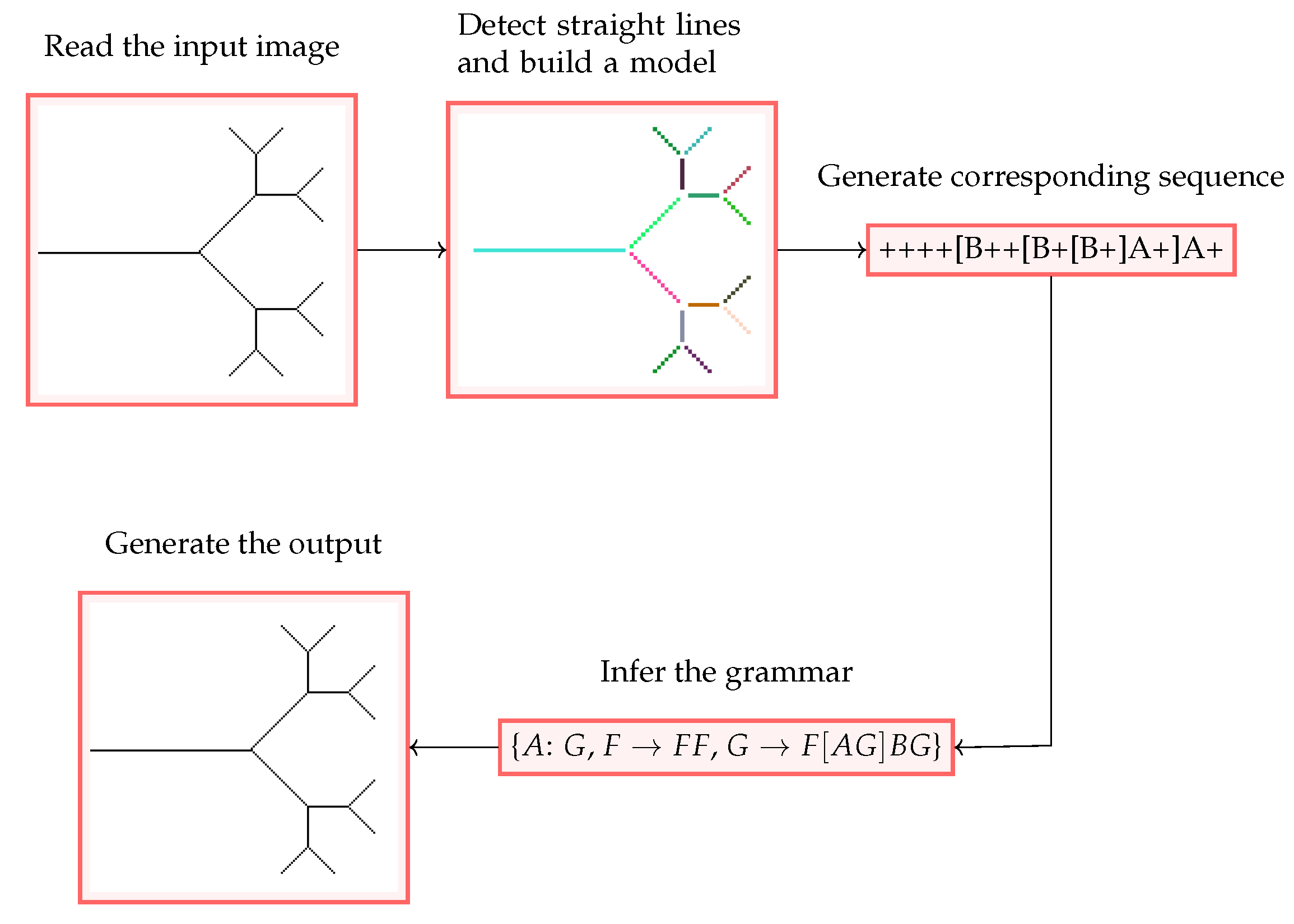
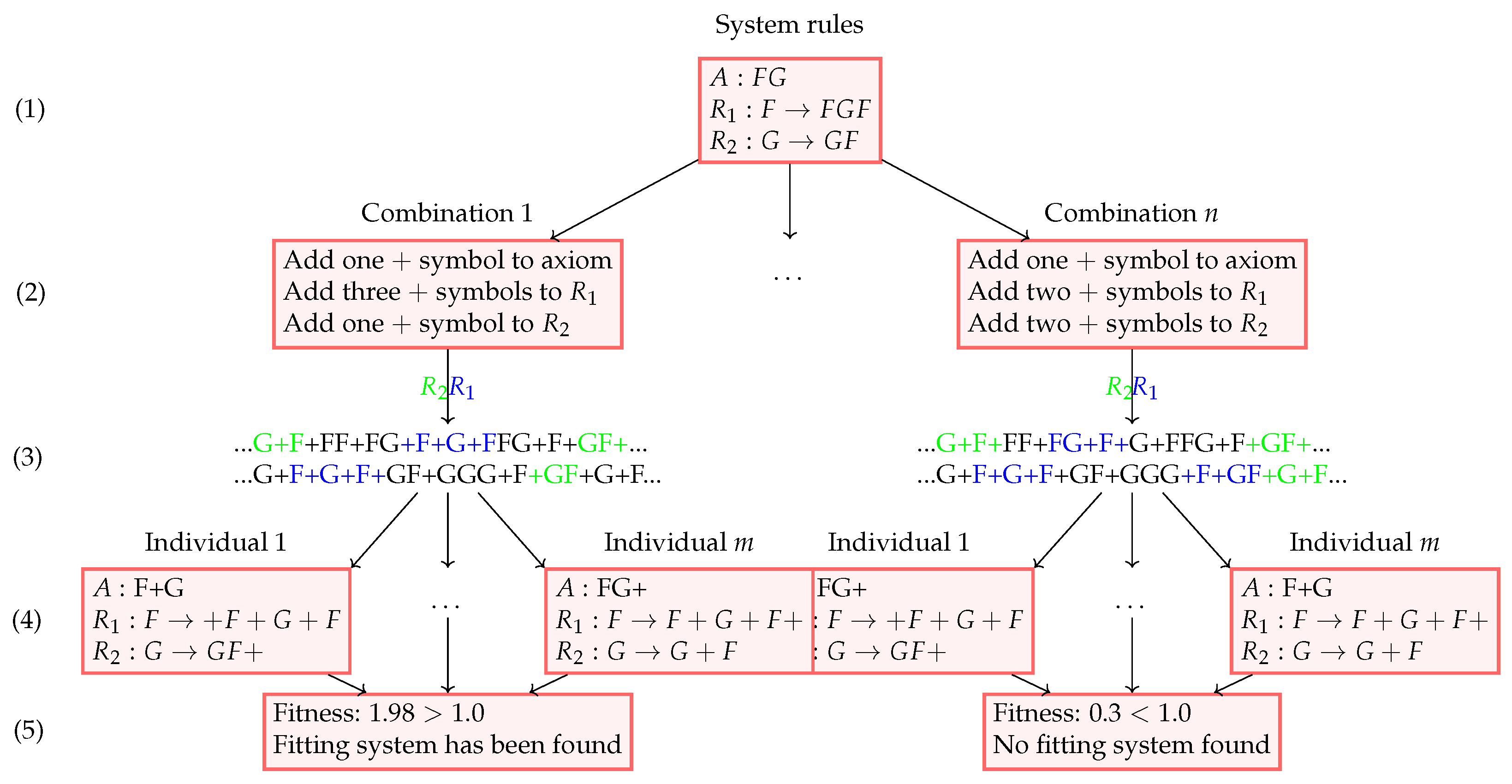
The proposed approach is to parse the input image into a sequence of symbols that describe the geometrical structure generated from an L-system and then use a GA to infer the system’s grammar (Figure 2). The respective steps of the proposed D0L-system induction method are described below.

2.6. Image Parsing

The parsing can be done using general line detection algorithms (like D-DBSCAN [23]), but the results are often not precise enough for this application; therefore, we have employed our line detection algorithm.
The process of parsing the image into an input sequence is divided into three steps. First, all of the straight lines are detected in the image. Then, all of these lines are connected, building a model of the structure in the image so in the last step we can generate a sequence that accurately describes this model.

2.6.1. Straight Line Detection

For usage in our algorithm, we defined a line as a set of continuous points, understood as pixels in an image, each neighbouring at most two other points. A point with more than two neighbours is treated as a line intersection, and a point with only one neighbour, an edge point, is considered a line end. The neighbourhood is based on the euclidean distance between points in the image—two points are neighbours if the distance between them is not greater than 2 , which is the largest distance between two touching pixels in an image.
To detect straight lines in the image, the procedure traverses the image looking for a pixel that has two neighbours and therefore belongs to a straight line according to its definition. Starting from this point, consecutive connected pixels are added to the detected line for as long as they have only two neighbours. The line detection ends when on both ends of the line the algorithm detects either an edge point or an intersection (multiple-neighbour point). Each visited point is also marked, so it is not under consideration when looking for the next lines.
One case that is not handled by the line definition is when a line changes direction. Two connected lines might conform to the definition and be detected as a single line even if they are clearly not the same line. The splitting of such lines is handled after the line detection process finishes. Given that a line is a set of points, to find a change of direction, we are looking for the largest continuous subsets of points that fit a linear model with some acceptable error.
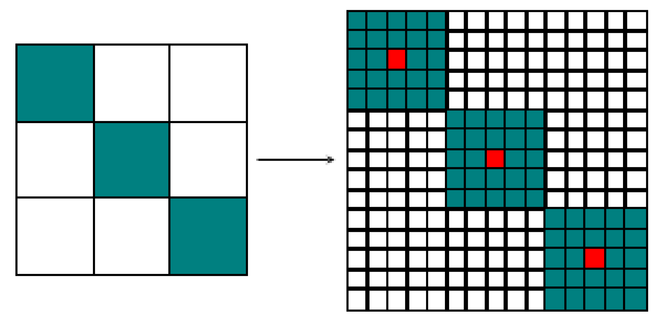
To check if a set of points fits a linear model, an algorithm based on a simple idea is used—if the subset contains points of a straight line, the line between the first and the last point goes through all of the remaining points. It takes the first and the last point of the subset and finds a linear model that fits those points. Afterwards, it checks whether the model fits the remaining points of the subset. A model fits a point when the distance between the point and the linear model is smaller than a specified acceptable error. However, when working with indexes of pixels in an image, the accuracy is often not enough to correctly match the line to the points. That is why the points are first cast into a virtual space with higher granularity, which is a parameter of the algorithm. For example, given a granularity of 2, a pixel is divided into a grid of 5 by 5 cells (Figure 3).
After casting each of the points to this virtual space, now a pixel matches the linear model if the distance from any of his cells to the linear model is smaller than the acceptable error. This effectively allows us to work with higher resolution than the original image and gives much more accurate results.
Due to inaccuracies in drawing straight lines, especially at the intersections of multiple lines, there are usually some points that could not be assigned to any of the lines. These points are grouped together with their unassigned neighbours and memorized into intersection groups for later use. They will be used during model building as connectors between lines.

2.6.2. Model Building

Before a model can be built from detected lines, two preprocessing steps must be made. We are looking for a non-parametric system, which means that every line must be of the same length. However, in the image, multiple lines can appear in consecutive order without changing direction, and the line detection algorithm will detect it as a single long line. The first pre-processing step takes care of this problem and splits long lines so that each line in the model is of the same length.
Because every symbol representing the “turn-by-angle” action needs to be associated with a specific angle, in the second pre-processing step, the information about all of the angles between the lines needs to be retrieved from the image. The drawn lines are only an approximation of actual straight lines; therefore, to calculate an angle between them, we need to apply some rounding and cannot achieve very high precision. The result of this step is a set of unique tilt angles rounded to the closest k degrees.
After the presented pre-processing steps, a model of the detected structure can be built. This is a recursive process that connects lines with their successors by finding the edge point of the line and then looking in the set of unused lines for one that is connected to it. A line is connected to an edge point when the edge point is a neighbour of one of its points. However, an edge point might not be connected to any line. In this case, we can search the set of intersection groups to check if the edge point is connected to any of them. If that is true, it means that the line connects to an intersection and will be connected to any other line that is also connected to this intersection.

2.6.3. Sequence Generation

The last step is the translation of generated model of a structure into a sequence of symbols. First, an alphabet needs to be generated. Some of the symbols are expected to always appear in an alphabet. Those include a draw forward (‘+’) symbol, and if the structure contains intersections, save the current position (‘[’) and return to the last saved position (‘]’) symbols since they are required to produce a branching structure. Some systems might use more than one draw-forward symbol; however, at this stage, it is not possible to deduce this, so a placeholder is used for every possible actual symbol. The last class of symbols that needs to be included in the alphabet is the turn symbols. During the pre-processing step, a set of all unique tilt angles is gathered, and a unique symbol is assigned for each value and added to the alphabet.
After creating the alphabet, a sequence can be generated. The algorithm traverses the structure model starting from the first line. For each straight line, a draw forward symbol is added to the sequence and the algorithm moves on to the next connected line. If there is a change of direction between the current and the next line before translating the next part of the model, an appropriate tilt-by-angle symbol is inserted. When the algorithm approaches an intersection, a save position symbol is inserted, and each branch is translated, returning to the previous position after finishing and moving on to the next branch. The branches are processed in the order of the smallest absolute value of the tilt angle. The return to the position symbol is not inserted at the end of the sequence since this information is redundant and does not appear in practical systems.

2.7. Grammar Inference

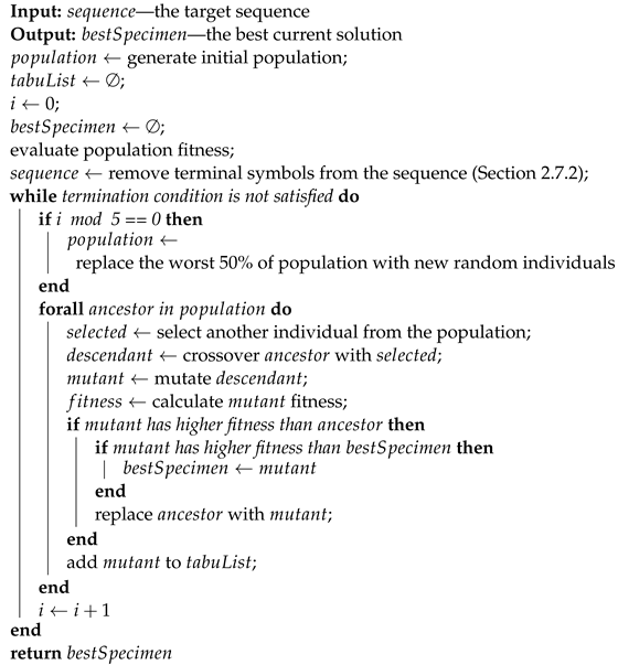
After parsing the input image into a sequence of symbols, an attempt at grammar inference can be made. There are many unknown variables, and the search space is large. A genetic algorithm is proposed (Algorithm 1), but first, two techniques used for space reduction need to be introduced.

2.7.1. Calculating Sequence Length at the nth Iteration of System

For a given alphabet V p = { σ 1 , σ 2 , , σ n } , the Parikh vector of a sequence w is a vector P w = [ | S σ 1 | , | S σ 2 | , , | S σ n | ] where the element | S σ i | contains the number of appearances of symbol σ i in this sequence. Let P r i denote a Parikh vector of the successor of the rule r i and P L i a Parikh vector of a sequence generated by a system in its ith iteration. Then, we can define a growth matrix
I = P r 1 P r 2 P r n .
which allows us to calculate the Parikh vector of the sequence generated by a system in any iteration, which will be essential for calculating offspring fitness. The sequence Parikh vector can be calculated as follows:
P L k I m = P L m + k .
Using a growth matrix, we can check if a set of rules ω can generate a sequence with a given Parikh vector P L m . To do this, we need to determine if there exists, for a given m, such a Parikh vector P L 0 that the Equation (2) is satisfied. If it does, then a system with rules ω and an axiom with a Parikh vector P L 0 can generate a sequence of the same length as the target sequence in m iterations. If such a vector does not exist, we can find a vector with the closest sequence length by solving an integer programming problem:
max P L 0 [ 1 ] , P L 0 [ 2 ] , , P L 0 [ n ] ,
i { 1 , , n } , P L n [ i ] P w [ i ]
Algorithm 1: L-system inference
Information 14 00343 i001

2.7.2. System Independence from Terminal Symbols

Let us say that S is an L-system with an alphabet containing two terminal and non-terminal symbols that generates a sequence L in the nth iteration. Knowing that a terminal character cannot be a base of a rule, we can notice that we can remove terminal symbols and analyze a more straightforward case [16]. If system S generates a sequence L and we remove terminal characters from the rules of S, it will still produce the same sequence without the terminal symbols. For example,
S : { A : F , F F + G + F , G G F G } L 2 = F+G+F+G-F-G+F+G+F S ^ : { A : F , F F G F , G G F G } L ^ 2 = FGFGFGFGF
We can see that excluding the terminal symbols sequences L 3 and L 3 ^ are equivalent. Thanks to this property during system inference, we can first solve a simpler problem without the terminal symbols and then gradually add the terminal symbols back to the system, obtaining subsequent partial solutions. The algorithm arrives at a full solution after restoring all of the terminal symbols. This requires more searches, but each has a significantly reduced search space.

2.7.3. Genetic Algorithm

The task to be solved by this algorithm is as follows: find a set of rewriting rules that, for some axiom, allows for the generation of the target sequence in the nth iteration. The individuals are encoded using Parikh vectors of rewriting rules. Before the start of the algorithm, all of the terminal symbols are removed from the target sequence in line with the logic from Section 2.7.2. Therefore, the individuals’ Parikh vectors contain only counts of non-terminal symbols.

Initial Population Generation

The exact number of rules is unknown; therefore, the population should contain individuals with different amounts. An m N ratio was adopted, where m represents the maximum amount of rules and N is the size of the population. For each class of systems, rules are generated randomly, with lengths ranging from 1 to a specified maximum length value k. Due to the high cost of the fitness function, the population size has to be kept low. This might cause all of the individuals to converge to the same local minima, which prevents the algorithm from exploring the whole search space. To solve this problem, the worse half of the population is replaced by new randomly generated offspring every five iterations.

Genetic Operators

This algorithm uses a typical crossover operator, with the offspring having some chance of receiving each rule from either of the parents regulated by the c r o s s o v e r R a t i o parameter. It needs to be noted that only parents with an identical rule count can be bred together. The mutation operator is implemented in the form of four independent operations—SWAP (swap the successors of two rules), ADD (add a random symbol to one of the rules), REMOVE (remove a random character from one of the rules with more than one symbol), and CHANGE (change one of the symbols in one of the rules into another). If an offspring is to be modified, each operation has an equal probability of being applied. In the case of L-systems, changing a single symbol rarely leads to a better result. That is why a memory mechanism has been introduced. Every visited solution is memorized, and if the future mutation results in a previously encountered state, the operator is repeatedly applied until a new solution is obtained. The selection operator picks a random partner for every individual in the population, with candidates with higher fitness having a better chance of being selected. The algorithm terminates when a complete solution is found or the maximum iteration count has been reached.

Fitness Function

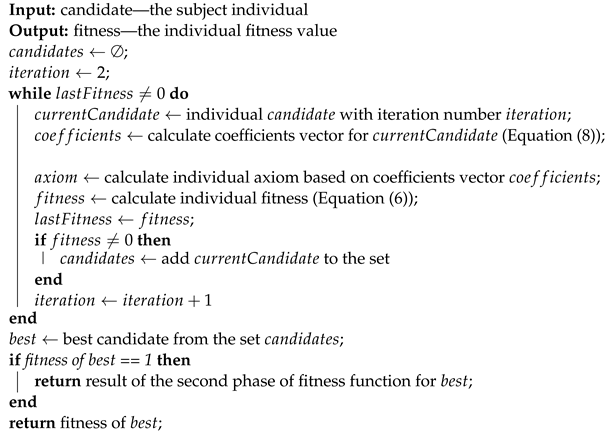
The selected fitness function executes in two phases. During the first stage (Algorithm 2), the sequence length is considered, and the fitness can reach a maximum value of 1.0, which signals that the generated sequence has reached the target length. If an individual reaches ultimate fitness for the first stage, the second phase begins, where terminal symbols are consecutively reinserted, and an exact sequence match is evaluated in each step. The fitness increases for each correctly inserted terminal character.
The first phase of the fitness calculation evaluates whether the individual can generate a sequence with the same length as the target sequence in N iterations. The closer the sequence length is to the target sequence length, the higher the fitness. The fitness of the individual for a given N can be evaluated using the method specified in Section 2.7.1 by calculating the coefficient vector:
I N = a 11 a 12 a 1 n a 21 a n 1 a n 2 a n n c = c 0 c 1 c n = a 11 + a 12 + + a 1 n a 21 + a 22 + + a 2 n a n 1 + a n 2 + + a n n ,
and solving an integer programming problem:
m a x ( c 0 x 0 + c 1 x 1 + + c n x n ) ,
0 c 0 x 0 + c 1 x 1 + + c n x n | L | ,
i { 0 , , n } , x i | L |
that gives a solution in the form of r = x 0 x 1 x n , which is a Parikh vector of the system axiom. Then the fitness of the individual is calculated as follows:
Fitness = 1.0 | L | i = 0 | r | c i x i | L | .
However, since N is unknown, we must check multiple values. For every system, there is an iteration number M for which finding a valid axiom is no longer possible, and a value of N = 1 is not practically useful; therefore, we have to check values of N in the range 2 ; M and find N with the highest fitness value as the final result.
Algorithm 2: Fitness function
Information 14 00343 i002
The second phase of the fitness calculation evaluates whether the individual can correctly generate a sequence that exactly matches the target sequence. The process runs in a few iterations, and in each one, a single terminal symbol is reinserted into the target sequence. Then, we are trying to find how to insert the new character into the rules and the axiom so that the system can generate the target sequence. The general outline of a single iteration is pictured in Figure 4. The initial state is the result of the previous iteration. For the sequences to match, they must contain the same number of each symbol. Therefore, there is a finite set of combinations in which we can insert the new character into the rules so that the Parikh vectors of the sequences are equal. In step 2, the algorithm calculates all of the possible combinations by calculating the coefficients vector W:
W = i = 1 k P A I i 1 = W 0 W 1 W n ,
and solving an integer programming problem:
W 0 x 0 + W 1 x 1 + + W n x n + x A = | L | ,
i { 0 , , n } , x i | L | ,
0 x A | L | ,
which gives us a set of vectors x 0 x 1 x n x A , where x n and x A is the occurrence count of terminal symbol in the nth rule and the axiom, respectively. Because the number of combinations can be large, we can take the simplest ten for the best results. Now we know how many symbols to insert but not where. To avoid exploring all of the possibilities, since the rules’ successors must appear in the target sequence, we can reduce the search space by only using the appropriate subsequences in the target sequence, which is done in step 3. From the found subsequences, in step 4, the algorithm generates a population for the GA. Since the axiom does not appear in the sequence, we only know the number of symbols to be added but not their positions; therefore, the symbols are randomly inserted. In the last step, a GA finds a system that can recreate the target sequence using the generated initial population.
A typical crossover operator has been employed, with the descendant receiving each rule from one of the parents according to a selected ratio. A mutation operator can permute non-terminal symbols of one or more rules and the system axiom. Individuals are picked for breeding using elitist selection, with the top 10% of the population moving on to the next generation unchanged. The chosen fitness function compares the generated sequence and target sequence symbol by symbol. If a character at a given position matches, the individual receives one point. It needs to be noted that the output of the image parsing algorithm contains only a single type of non-terminal symbol; therefore, every non-terminal character receives a point for matching with it. The final fitness is a ratio between received points and total sequence length. Because the target sequences are usually very long, an optimization was applied, where only the first 100 symbols are compared, and only if those match the rest of the string is validated. When the entire sequence is correctly matched, the individual can increase their fitness value by a maximum of 1.0, relative to the simplicity of the system evaluated as:
F i t n e s s = | L | | A | | L | .
The algorithm terminates when it finds a solution or reaches the maximum iteration count.
If we are looking for a single rule system, an additional optimization can be applied. Since the system axiom must start with a non-terminal symbol and a single rule cannot start with a terminal character, we can conclude that any generated sequence must begin with the rule’s successor. Therefore, in step 3, instead of searching the whole string for matches, we can analyze only the first subsequence of adequate length and avoid steps 4 and 5 since there is only one matching subsequence, and we can outright check if it generates a correct sequence.

3. Results

Multiple L-systems found in the literature were selected as the example inputs to test the algorithm’s efficiency. To be picked, the grammar could not have contained non-graphical symbols in its alphabet and had to generate a structure with no intersecting lines. The following systems were used: Koch Island [6,12,24], Koch Snowflake [24], Koch Curve [25], Barnsley Fern [6,13], Sierpiński Triangle [6], and Binary Tree [13]. From each selected system, an example image was generated by our plotting program and used during testing (such an approach is called grammar inference on synthetic images [26]). All of the tests were run on an AMD Ryzen 9 3900X PC with 16GB RAM. GPU acceleration and multi-threading were not used.

3.1. Grammar Inference

The tests for the provided examples succeeded in every case, including those successfully used in [13]. The initial population of 20 was used, with a mutation probability of 0.7 and a crossover ratio of 0.5. These parameters were selected during the initial experiments. The inferred systems were an exact match to the originals, with some minor notation differences that did not alter the system functionality.
The algorithm was also tested using examples used by the LGIN tool [11], and the results were compared. A solution was found in every case. However, the runtime was longer. It was to be expected since the LGIN tool uses an arithmetic approach instead of a search algorithm, which allows for faster execution but requires multiple constraints to be applied—only one or two rule systems can be inferred, with known axiom and rule count.
To compare our algorithm to the approach of Runqiang et al. [14], we used the same two examples with one and two rules, with the single-rule L-system being an equivalent of the Ex01 system from the LGIN test suite and the second system being given as:
{ A : X , F F F , X F [ + X ] F [ X ] X } .
The original algorithm found a solution in every run for the first system and in 66% of the runs for the second system. Meanwhile, our approach found a solution for both systems in every run. Moreover, our algorithm ran for fewer iterations than the original one (Table 1).

3.2. More Complex Systems

The main advantage of our approach over the related arithmetic and heuristic algorithms described in Section 2.4 is its ability to work on systems with more than two rules. To test this capability, a system S 3 with three rewriting rules from Section 2.1 was used, and our algorithm successfully inferred the original grammar. Even though it took longer than for the simpler systems—1105 iterations in 25 min, it is a significant improvement over the mentioned algorithms that infer grammars with two rules at most.

3.3. Runtime Distribution

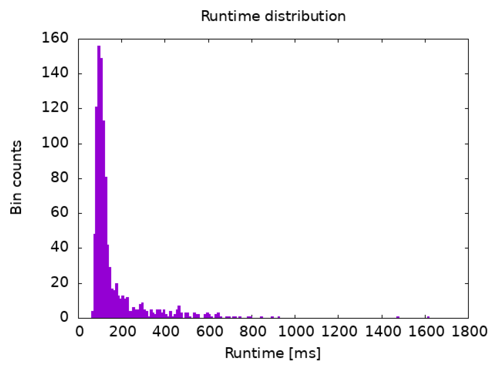
To test the replicability of our results, runtime distribution for the GA has been tested on systems with one and two rewriting rules. Test examples were taken from [14]. As seen in Figure 5, for a single rule system, most algorithm executions ran for a similar amount of time, around 100 ms, with very few stragglers that ran for more than 600 ms. For a system with two rules (Figure 6), we can notice similar behavior. However, here, we can see that a significant amount of runs finished quickly, meaning the initial population already contained a candidate with very high fitness. This lets us conclude that the algorithm has a low tendency to get stuck in areas of search space containing candidates with low fitness.

3.4. Koch Island

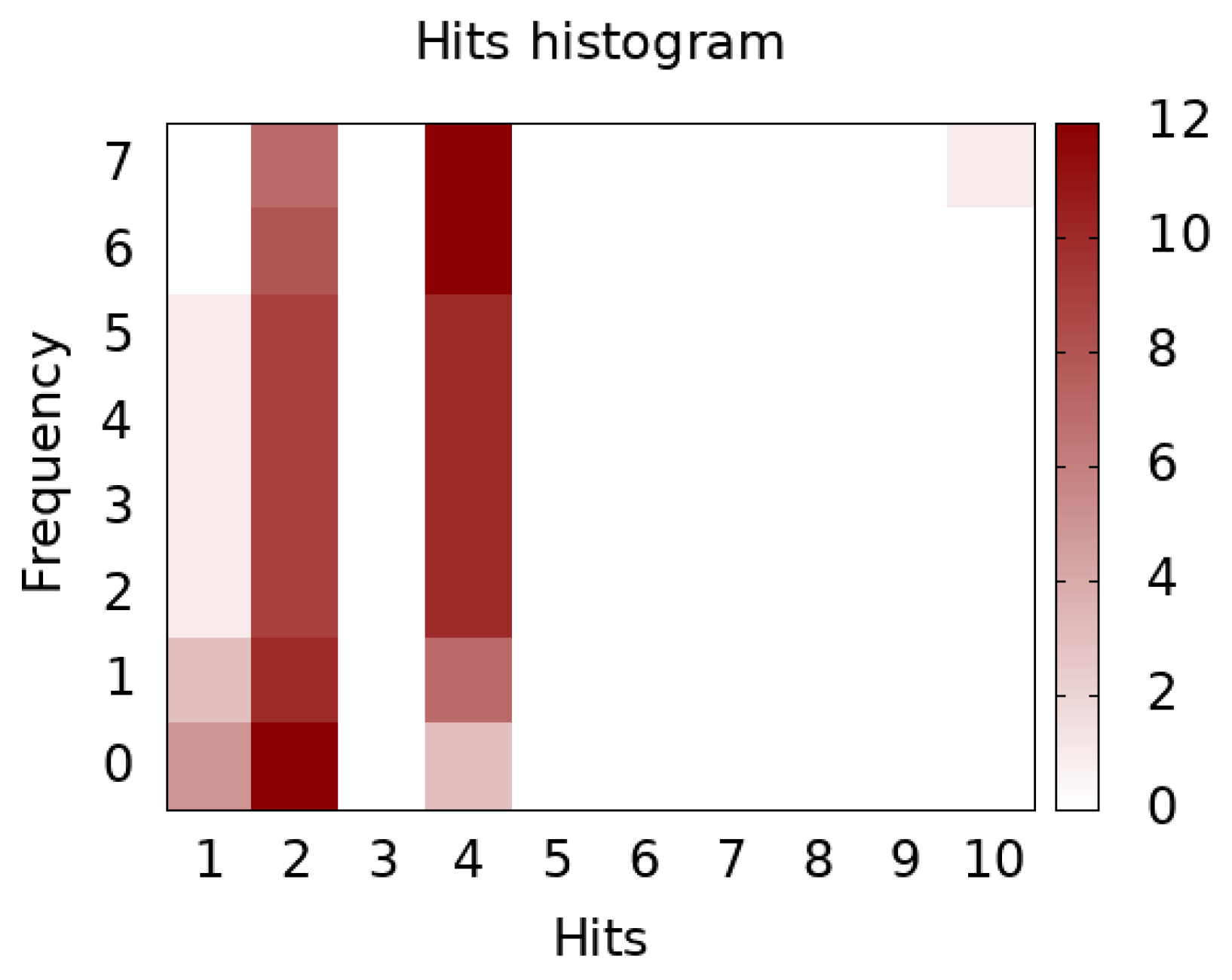
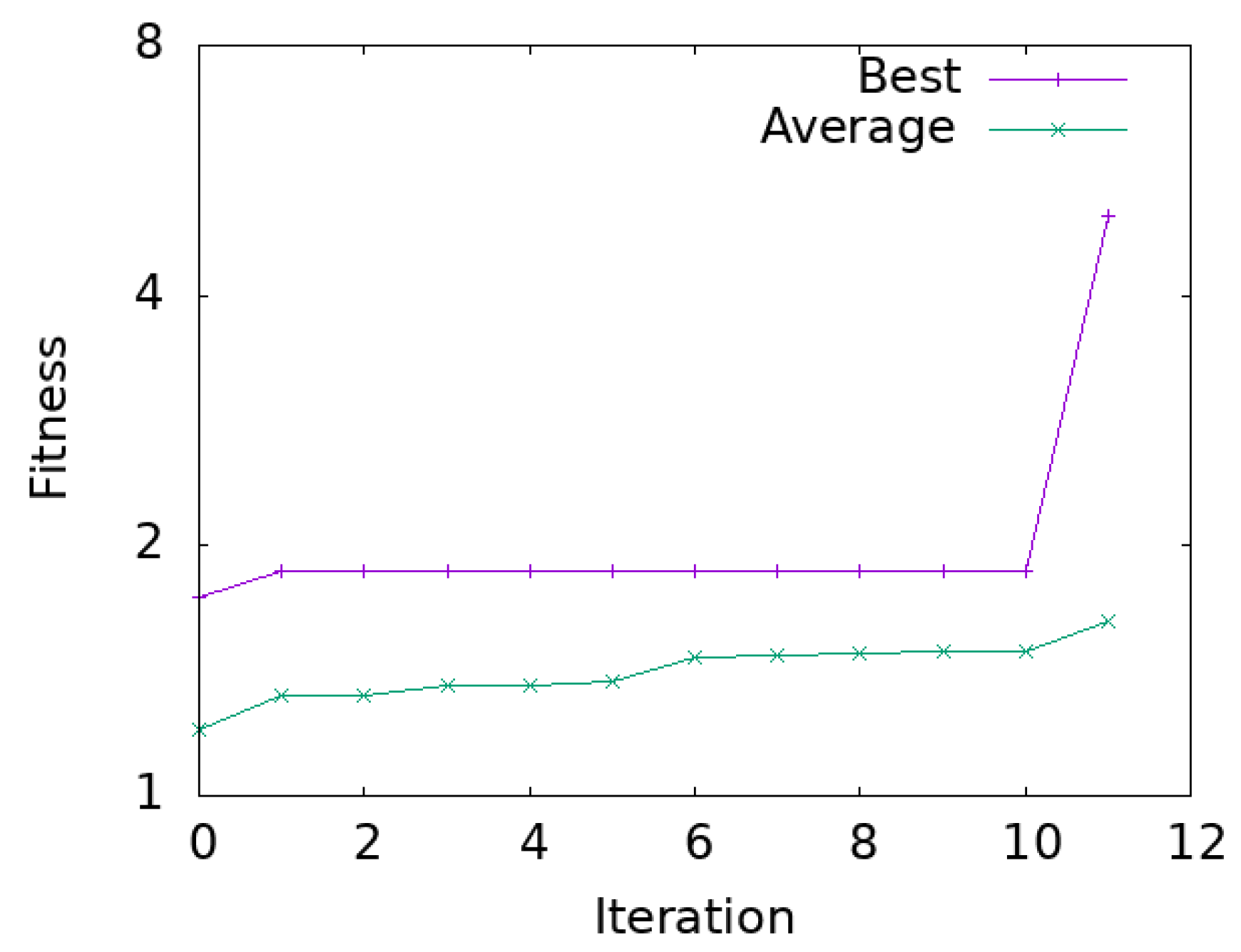
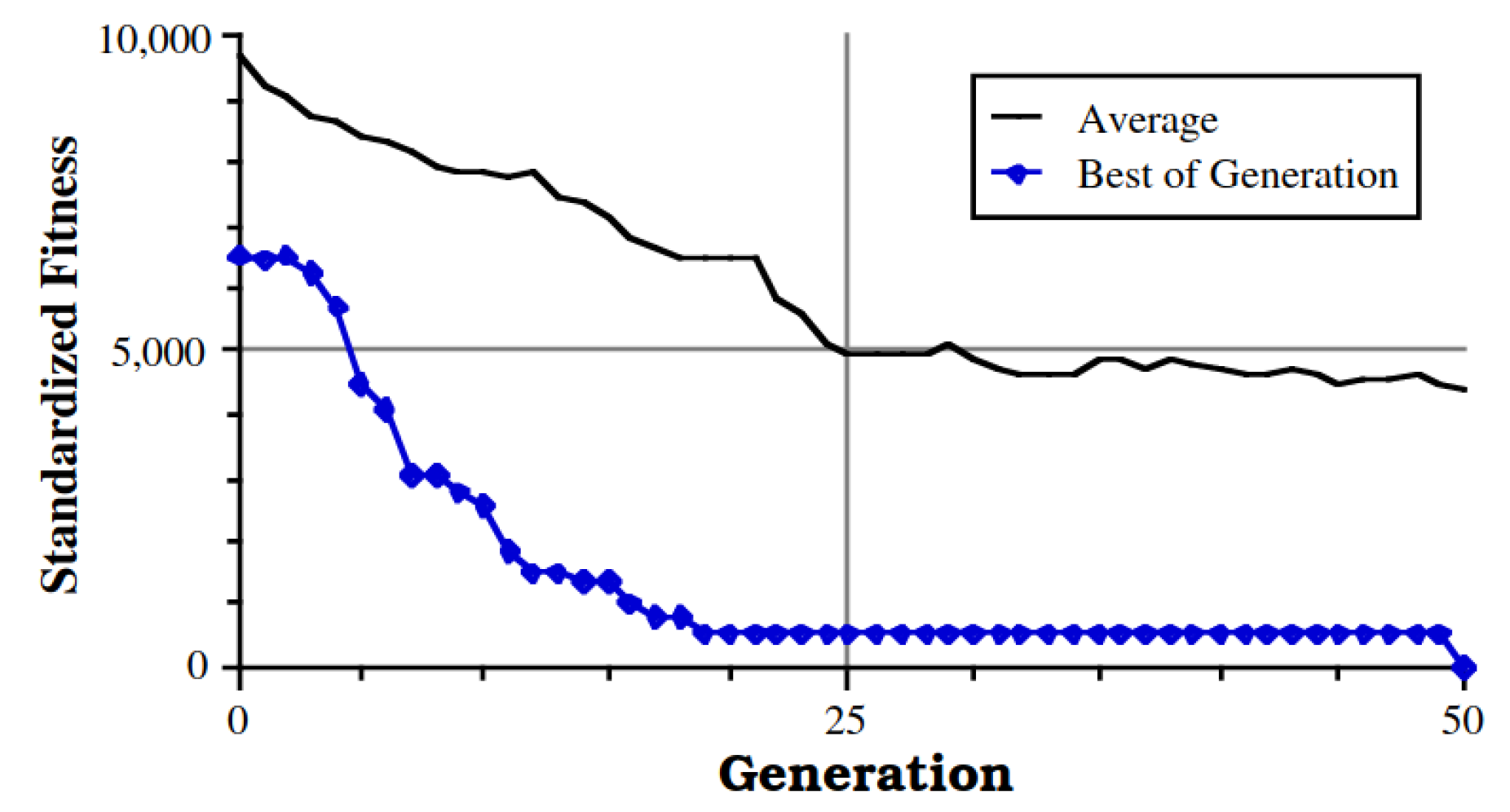
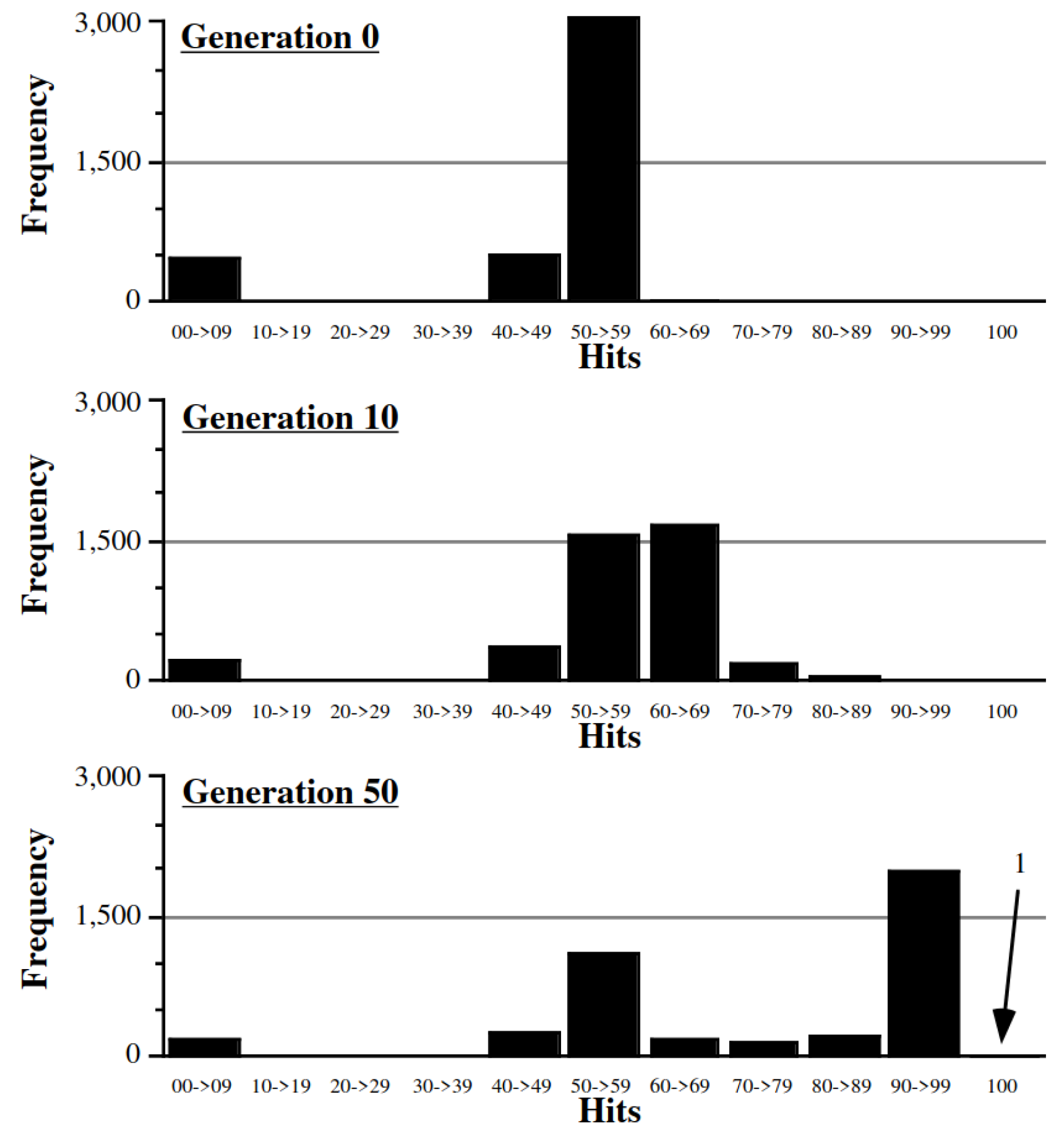
The effectiveness of the proposed algorithm was compared to the genetic programming method developed in [12]. It was one of the first attempts at inferring D0L-systems from a single sequence. Since then, multiple new solutions have been proposed. However, it is one of the better-documented articles, providing various performance metrics, which allow for a comprehensive comparison. The first difference in the results can be seen in the initial population generation. In the article mentioned above, it is stated that the members of the initial population of 4000 are not very good on average, with most placed around the middle of the fitness scale and the worst 12% of the population having the highest possible (the worst) fitness value. In our proposed algorithm, the population is much smaller; the tests were run using only 20 individuals. However, the generation is more effective—out of 1000 executed tests, only 32.7% of them required more than one iteration to reach a solution. Looking at the heatmap that shows the progress of hits histograms [12] (Figure 7) and changes of best and average fitness (Figure 8), we can notice that while in Koza’s algorithm the progress is very steady and consistent (Figure 9 and Figure 10), in our case, it is slower but has a tendency to take more significant leaps in quality.

3.5. Genetic Programming Using BNF Grammar

Finally, a comparison to the algorithm from the article by D. Beaumont and A. Stepney was made [15]. For this purpose, two example L-systems were used. The first one has a single rule and is given as
{ A F , F F [ + F ] F [ F ] F } .
The second one is equivalent to the Ex04Y system used for tests by the LGIN tool. In the first case, both algorithms arrived at a solution; although the compared algorithm returned multiple solutions, some of them very long or containing redundant symbols. In the second case, our algorithm managed to find a correct system every time; meanwhile, the compared algorithm achieved the same feat in only 2 in 200 test runs. The runtime was also much shorter; on average, the compared algorithm ran for several CPU-days for each test and required 891 iterations. Meanwhile, our algorithm completed the whole test suite of 30 runs in around 1 h and found a solution on average in 35 iterations.

3.6. Crossover between Individuals with Different Rule Counts

Since the selected crossover function operates only on individuals with the same rule count, two modifications have been tested. The main issue with the crossover between individuals with different rule counts is that individuals with more rules will have a larger alphabet and use symbols that are not valid for those with fewer rules. Therefore, the first modification allowed for a crossover when the second individual had the same amount or fewer rules as the main individual. This resulted in a slightly worse performance. The tests consisted of running the inference algorithm on System A from Section 3.1 for 1000 iterations. The modified crossover function resulted in an algorithm average runtime of 166.42 ms, while the original function achieved an average runtime of 161.04 ms.
The second modification further relaxed the constraints and allowed crossover between individuals with any rule count. To achieve this, a post-processing step had to be added, which, if the second individual had more rules, replaced the excess symbols with a random symbol from the smaller individual alphabet. This resulted in worse performance than the previous modification, with an average runtime of 169.84 ms. Overall, the crossover constrained to individuals with the same rule count seems to work the best, possibly because the rules already fit for this class of systems.

3.7. Comparison with Generational GA Approach

Our proposed solution uses a steady-state GA (SSGA) algorithm [27] in which only individuals that are better than their parents are inserted into the population. This approach has been compared to a generational GA (GGA) algorithm that replaces each generation’s whole population. The comparison was made using the same tests as in Section 3.6. The results show a promising improvement, with the GGA algorithm achieving an average runtime of 147.5 ms compared to the 161.04 ms of the SSGA algorithm. This shows that enhancements to the breeding scheme can introduce even better performance of the inference algorithm.

4. Discussion

An algorithm for image-based grammatical inference of deterministic, context-free L-systems was proposed. The effectiveness of this approach was compared to multiple test results of comparable algorithms and tested using our examples. The results show that the algorithm performs better than existing heuristic techniques and can find solutions for the same problems as the arithmetic approaches. A significant improvement over previous methods has been made, proving that solving inference problems for systems with more than two rules is possible. However, further research is still needed. The GA’s fitness function is effective but computationally costly, which implies that optimizations in this area could lead to the development of an algorithm that can solve systems with even higher rule count in a reasonable time. Further improvements to the fitness function or the encoding scheme should also be researched, studying whether fitness progress can be faster and more gradual, eliminating the frequent large jumps or decreasing the number of runs that take much longer than average. Some of the compared algorithms work faster under certain conditions, and incorporating some of their ideas into the fitness function might lead to quicker computation. Most importantly, this research shows that further advancements in single-sequence grammatical inference for D0L-systems are possible, and new solutions can provide better results, solving even more complex systems.

Author Contributions

Conceptualization, M.Ł. and O.U.; methodology, M.Ł.; software, M.Ł.; validation, M.Ł.; formal analysis, M.Ł.; investigation, M.Ł.; resources, M.Ł. and O.U.; data curation, M.Ł.; writing—original draft preparation, M.Ł. and O.U.; writing—review and editing, M.Ł. and O.U.; visualization, M.Ł.; supervision, O.U.; and project administration, O.U. All authors have read and agreed to the published version of the manuscript.

Funding

This research received no external funding.

Data Availability Statement

Not applicable.

Conflicts of Interest

The authors declare no conflict of interest.

References

  1. Komosinski, M.; Adamatzky, A. Artificial Life Models in Software; Springer Science & Business Media: Berlin/Heidelberg, Germany, 2009. [Google Scholar]
  2. Langton, C. Artificial Life: Proceedings of an Interdisciplinary Workshop on the Synthesis and Simulation of Living Systems; Routledge: Oxfordshire, UK, 2019. [Google Scholar]
  3. Rozenberg, G.; Salomaa, A. The Mathematical Theory of L Systems; Academic Press: Cambridge, MA, USA, 1980. [Google Scholar]
  4. Parish, Y.I.; Müller, P. Procedural modeling of cities. In Proceedings of the 28th Annual Conference on Computer Graphics and Interactive Techniques, Los Angeles, CA, USA, 12–17 August 2001; pp. 301–308. [Google Scholar]
  5. Manousakis, S. Non-standard Sound Synthesis with L-systems. Leonardo Music J. 2009, 19, 85–94. [Google Scholar] [CrossRef]
  6. Prusinkiewicz, P. Graphical applications of L-systems. In Proceedings of the Graphics Interface, Vancouver, BC, Canada, 26–30 May 1986; Volume 86, pp. 247–253. [Google Scholar]
  7. De la Higuera, C. Grammatical Inference: Learning Automata and Grammars; Cambridge University Press: Cambridge, UK, 2010. [Google Scholar]
  8. Whitley, D. An overview of evolutionary algorithms: Practical issues and common pitfalls. Inf. Softw. Technol. 2001, 43, 817–831. [Google Scholar] [CrossRef]
  9. Abdel-Basset, M.; Abdel-Fatah, L.; Sangaiah, A.K. Metaheuristic algorithms: A comprehensive review. In Computational Intelligence for Multimedia Big Data on the Cloud with Engineering Applications; Academic Press: Cambridge, MA, USA, 2018; pp. 185–231. [Google Scholar]
  10. Santos, E.; Coelho, R.C. Obtaining l-systems rules from strings. In Proceedings of the 2009 3rd Southern Conference on Computational Modeling, Rio Grande, Brazil, 23–25 November 2009; IEEE: Piscataway, NJ, USA, 2009; pp. 143–149. [Google Scholar]
  11. Nakano, R.; Yamada, N. Number theory-based induction of deterministic context-free L-system grammar. In Proceedings of the International Conference on Knowledge Discovery and Information Retrieval, Valencia, Spain, 25–28 October 2010; SCITEPRESS: Setúbal, Portugal, 2010; Volume 2, pp. 194–199. [Google Scholar]
  12. Koza, J.R. Discovery of rewrite rules in Lindenmayer systems and state transition rules in cellular automata via genetic programming. In Proceedings of the Symposium on Pattern Formation (SPF-93), Claremont, CA, USA, 13 February 1993; Citeseer: Princeton, NJ, USA, 1993; pp. 1–19. [Google Scholar]
  13. Eszes, T.; Botzheim, J. Applying Genetic Programming for the Inverse Lindenmayer Problem. In Proceedings of the 2021 IEEE 21st International Symposium on Computational Intelligence and Informatics (CINTI), Budapest, Hungary, 18–20 November 2021; IEEE: Piscataway, NJ, USA, 2021; pp. 000043–000048. [Google Scholar]
  14. Runqiang, B.; Chen, P.; Burrage, K.; Hanan, J.; Room, P.; Belward, J. Derivation of L-system models from measurements of biological branching structures using genetic algorithms. In Developments in Applied Artificial Intelligence: 15th International Conference on Industrial and Engineering Applications of Artificial Intelligence and Expert Systems IEA/AIE 2002, Cairns, Australia, 17–20 June 2002; Springer: Cham, Switzerland, 2002; pp. 514–524. [Google Scholar]
  15. Beaumont, D.; Stepney, S. Grammatical Evolution of L-systems. In Proceedings of the 2009 IEEE Congress on Evolutionary Computation, Trondheim, Norway, 18–21 May 2009; IEEE: Piscataway, NJ, USA, 2009; pp. 2446–2453. [Google Scholar]
  16. Bernard, J.; McQuillan, I. New techniques for inferring L-systems using genetic algorithm. In Proceedings of the Bioinspired Optimization Methods and Their Applications: 8th International Conference, BIOMA 2018, Paris, France, 16–18 May 2018; Springer: Cham, Switzerland, 2018; pp. 13–25. [Google Scholar]
  17. Bernard, J.; McQuillan, I. A fast and reliable hybrid approach for inferring L-systems. In Proceedings of the ALIFE 2018: The 2018 Conference on Artificial Life, Tokyo, Japan, 23–27 July 2018; MIT Press: Cambridge, MA, USA, 2018; pp. 444–451. [Google Scholar]
  18. Bernard, J.; McQuillan, I. Techniques for inferring context-free Lindenmayer systems with genetic algorithm. Swarm Evol. Comput. 2021, 64, 100893. [Google Scholar] [CrossRef]
  19. McQuillan, I.; Bernard, J.; Prusinkiewicz, P. Algorithms for inferring context-sensitive L-systems. In Proceedings of the Unconventional Computation and Natural Computation: 17th International Conference, UCNC 2018, Fontainebleau, France, 25–29 June 2018; Springer: Cham, Switzerland, 2018; pp. 117–130. [Google Scholar]
  20. Bernard, J.; McQuillan, I. Inferring stochastic L-systems using a hybrid greedy algorithm. In Proceedings of the 2018 IEEE 30th International Conference on Tools with Artificial Intelligence (ICTAI), Volos, Greece, 5–7 November 2018; IEEE: Piscataway, NJ, USA, 2018; pp. 600–607. [Google Scholar]
  21. Bernard, J.; McQuillan, I. Stochastic L-system inference from multiple string sequence inputs. Soft Comput. 2022, 27, 6783–6798. [Google Scholar] [CrossRef]
  22. Bernard, J.; McQuillan, I. Inferring Temporal Parametric L-systems Using Cartesian Genetic Programming. In Proceedings of the 2020 IEEE 32nd International Conference on Tools with Artificial Intelligence (ICTAI), Baltimore, MD, USA, 9–11 November 2020; IEEE: Piscataway, NJ, USA, 2020; pp. 580–588. [Google Scholar]
  23. Lee, S.; Hyeon, D.; Park, G.; Baek, I.-j.; Kim, S.W.; Seo, S.W. Directional-DBSCAN: Parking-slot detection using a clustering method in around-view monitoring system. In Proceedings of the 2016 IEEE Intelligent Vehicles Symposium (IV), Gothenburg, Sweden, 19–22 June 2016; IEEE: Piscataway, NJ, USA, 2016; pp. 349–354. [Google Scholar]
  24. Prusinkiewicz, P.; Hanan, J. Lindenmayer Systems, Fractals, and Plants; Springer Science & Business Media: Berlin/Heidelberg, Germany, 2013; Volume 79. [Google Scholar]
  25. Purnomo, K.D.; Sari, N.P.W.; Ubaidillah, F.; Agustin, I.H. The construction of the Koch curve (n, c) using L-system. In AIP Conference Proceedings; AIP Publishing LLC: Woodbury, NY, USA, 2019; Volume 2202, p. 020108. [Google Scholar]
  26. Guo, J.; Jiang, H.; Benes, B.; Deussen, O.; Zhang, X.; Lischinski, D.; Huang, H. Inverse procedural modeling of branching structures by inferring L-systems. ACM Trans. Graph. (TOG) 2020, 39, 1–13. [Google Scholar] [CrossRef]
  27. Syswerda, G. A study of reproduction in generational and steady-state genetic algorithms. In Foundations of Genetic Algorithms; Elsevier: Amsterdam, The Netherlands, 1991; Volume 1, pp. 94–101. [Google Scholar]
Figure 1. A structure generated by the S 3 system in the third iteration.
Information 14 00343 g001
Figure 2. General Outline of the Grammar Inference Algorithm.
Information 14 00343 g002
Figure 3. A few line points cast into virtual space with granularity = 2.
Information 14 00343 g003
Figure 4. General outline of a single iteration of the second phase of the fitness function.
Information 14 00343 g004
Figure 5. Runtime distribution for single rule system.
Information 14 00343 g005
Figure 6. Runtime distribution for two rule system.
Information 14 00343 g006
Figure 7. Hits heatmap of our algorithm.
Information 14 00343 g007
Figure 8. Fitness progression of our algorithm.
Information 14 00343 g008
Figure 9. Fitness progression of the algorithm from [12].
Information 14 00343 g009
Figure 10. Hits histograms of the algorithm from [12].
Information 14 00343 g010
Table 1. Results of comparison with the algorithm from [14].
Iteration Count of Own AlgorithmIteration Count of GA from [14]
MinimumAverageMaximum σ 1 MinimumAverageMaximum
System A11.751.34110.838
System B831.57030.793253.597
1 Standard deviation.
Disclaimer/Publisher’s Note: The statements, opinions and data contained in all publications are solely those of the individual author(s) and contributor(s) and not of MDPI and/or the editor(s). MDPI and/or the editor(s) disclaim responsibility for any injury to people or property resulting from any ideas, methods, instructions or products referred to in the content.